---

Stony Brook IMS Preprint #1992/11

arXiv:math/9207220v1 [math.DS] 25 Jul 1992Stony Brook IMS Preprint #1992/11July 1992Local Connectivity of Julia Sets: Expository Lectures.J. MilnorStony Brook, July 1992Contents§1.

Local Connectivity of Quadratic Julia Sets(following Yoccoz) . .

. .

. .

. .

. .

. .

. .

. .

. .

. .

. .

. .

. .

. .

. .2§2.

Polynomials for which All But One of the Critical Orbits Escape(following Branner and Hubbard) . .

. .

. .

. .

. .

. .

. .

. .

. .

. .

. .

. 17§3.

An Infinitely Renormalizable Non Locally Connected Julia Set(following Douady and Hubbard). .

. .

. .

. .

. .

. .

. .

. .

. .

. .

. .

. 30Appendix: Length-Area-Modulus Inequalities .

. .

. .

. .

. .

. .

. .

. .

. .

. .

. 36Errata .

. .

. .

. .

. .

. .

. .

. .

. .

. .

. .

. .

. .

. .

. .

. .

. .

. .

. .

42References. .

. .

. .

. .

. .

. .

. .

. .

. .

. .

. .

. .

. .

. .

. .

. .

. .

. 45IntroductionThe following notes provide an introduction to recent work of Branner, Hubbard and Yoccoz on thegeometry of polynomial Julia sets.

They are an expanded version of lectures given in Stony Brook in Spring1992. I am indebted to help from the audience.Section 1 describes unpublished work by J.-C. Yoccoz on local connectivity of quadratic Julia sets.

Itpresents only the “easy” part of his work, in the sense that it considers only non-renormalizable polynomials,and makes no effort to describe the much more difficult arguments which are needed to deal with localconnectivity in parameter space. It is based on second hand sources, namely Hubbard [Hu1] together withlectures by Branner and Douady.

Hence the presentation is surely quite different from that of Yoccoz.Section 2 describes the analogous arguments used by Branner and Hubbard [BH2] to study higher degreepolynomials for which all but one of the critical orbits escape to infinity. In this case, the associated Julia setJ is never locally connected.

The basic problem is rather to decide when J is totally disconnected. ThisBranner-Hubbard work came before Yoccoz, and its technical details are not as difficult.

However, in thesenotes their work is presented simply as another application of the same geometric ideas.Chapter 3 complements the Yoccoz results by describing a family of examples, due to Douady and Hub-bard (unpublished), showing that an infinitely renormalizable quadratic polynomial may have non-locally-connected Julia set. An Appendix describes needed tools from complex analysis, including the Gr¨otzschinequality.We will assume that the reader is familiar with the basic properties of Julia sets and the Mandelbrotset.

(For general background, see for example [Be], [Br2], [D1], [D2], [EL], [L1], as well as the brief outlinein §3.) In particular, we will make use of external rays for a polynomial Julia set J(f) ⊂C .

(Compare[DH1], [DH2], [M2], [GM]. )1

§1. Local Connectivity of Quadratic Julia Sets (following Yoccoz).This section will prove the following.Theorem 1.

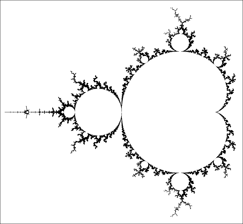
If fc(z) = z2 + c is a quadratic polynomial such that:(1) the Julia set J(fc) is connected,(2) both fixed points are repelling, and(3) fc is not renormalizable1then J(fc) is locally connected.In terms of the familiar parameter space picture for the family of quadratic maps fc(z) = z2 + c ,Condition (1) says that the parameter value c belongs to the Mandelbrot set M , while (2) says that cdoes not belong to the closure of the central region bounded by the cardioid, and (3) says that c does notbelong to any one of the many small copies of M which are scattered densely around the boundary of M . (Compare Figure 1.

)Figure 1. Boundary of the Mandelbrot set M , and a detail of the one-third limb showing severalsmall copies of M .Remarks: The proof will give much more, since it will effectively describe the Julia set by a newkind of symbolic dynamics.

With a little more work, the Yoccoz method can also deal with the finitelyrenormalizable case. Since the case of a map with attracting or parabolic fixed point had been understoodmuch earlier [DH2], we see that Conditions (2) and (3) can be actually replaced by the following weaker pairof conditions:(2′) f has no irrationally indifferent periodic points (Cremer or Siegel points), and(3′) f is not infinitely renormalizable.These modified Conditions (1), (2′) and (3′) are all essential.

In fact,1 For the definition of renormalizability, see Figure 10 and the associated discussion.2

(1): For c ̸∈M the Julia set J(fc) is a Cantor set, which is certainly not locally connected. (2′) : Sullivan and Douady showed that a polynomial Julia set with a Cremer point is never locallyconnected.

(Compare [Su], [D1], [M2]. For a more explicit description of non local connectivity, see [Sø].

)Similarly, Herman has constructed quadratic polynomials with a Siegel disk having no critical point on itsboundary. The corresponding Julia set cannot be locally connected.

(See [He,§17.1], [D1,II,5], [D4]. )(3′) : In §3, following unpublished work by Douady and Hubbard, we will describe infinitely renormal-izable polynomials for which J is not locally connected.Thus the sharpened version of Theorem 1 comes fairly close to deciding exactly which quadratic poly-nomial Julia sets are locally connected.

Yoccoz has also proved a corresponding result in parameter space:For c in the Mandelbrot set M , if the polynomial fc(z) = z2 + c is not infinitely renormalizable, then Mis locally connected at c . For varied proofs of this more difficult result, see [Hu2], [HF], [K].Figure 2.

Julia set for f(z) = z2 + i, showing the Yoccoz puzzles of depth zero andone. Here q = 3.

The 1/7 , 2/7 and 4/7 rays land at the fixed point α.The Yoccoz jigsaw puzzle. The proof of Theorem 1 begins as follows.

If a connected quadratic Juliaset has two repelling fixed points, then one fixed point (to be called β ) is the landing point of the zero externalray, and the other (called α ) is the landing point of a cycle of q external rays, where q ≥2 . (Compare [M2],[Pe].

)Let0 = c0 7→c1 7→· · · be the critical orbit.The Yoccoz puzzle of depth zero consists of q piecesP0(c0) , P0(c1) , . .

. , P0(cq−1) which are obtained by cutting the region G ≤1 along the q external rayslanding at α .

Here G is the canonical potential function. The various pieces have been labeled so that eachP0(ci) contains the post-critical point ci = f ◦i(0) .Inductive Construction: If P (1)d, .

. .

, P (m)dare the puzzle pieces of depth d , then the connectedcomponents of the sets f −1(P (i)d ) are the puzzle pieces P (j)d+1 of depth d + 1 . As an example, there arealways 2q −1 pieces of depth one.

These consist of q pieces P1(c0) , P1(c1) , . .

. , P1(cq−1) which touchat the fixed point α , together with q −1 additional pieces P1(−c1) , .

. .

, P1(−cq−1) which touch at thepre-image −α .The Main Problem: Let z ∈J(z) be any point whose forward orbit never hits1 the fixed point α ,1 The slight modifications of the argument needed to deal with the case f ◦d(z) = α are described near3

and let Pd(z) be the unique puzzle piece of depth d which contains this point z , so thatP0(z) ⊃P1(z) ⊃P2(z) ⊃· · · .Does the intersection Td Pd(z) consist of the single point z ?The associated annuli. Let Pd(z) ⊃Pd+1(z) be the puzzle pieces of two consecutive depths containingsome given z ∈J(f) .

If we are lucky, the smaller puzzle piece Pd+1(z) will be contained in the interior ofPd(z) . In this case the differenceAd(z) = interior(Pd(z))∖Pd+1(z)is an annulus, whose modulus mod Ad(z) is a positive real number.

(Compare the Appendix.) For examplein Figure 2 the annulus A0(−c1) has positive modulus.

On the other hand, it may happen that Pd+1(z)intersects the boundary of Pd(z) . In this case we describe Ad(z) as a degenerate annulus, and define itsmodulus to be zero.

For example, in Figure 2 the “annulus” A0(0) around the critical point is degenerate.ModifiedMainProblem(BrannerandHubbard):Givenapointz∈J(f) ,is the sum Pd mod Ad(z) infinite? If so, using the Gr¨otzsch inequality, it is not difficult to prove thatthe intersection T Pd(z) consists of the single point z .

(See Appendix. )Figure 3.

Critical, semi-critical and off-critical annuli (left), and a “child” (right).Note that f carries any puzzle piece Pd(z) of depth d > 0 onto Pd−1(f(z)) . This mapPd(z) →Pd−1(f(z))is either a conformal isomorphism or a two-fold branched covering according as Pd(z) does ordoes not contain the critical point.Definition.Wedescribeanannulusasbeingeithersemi-criticalorcriticaloroff-critical according as the critical point belongs to the annulus itself or to the bounded or the unboundedcomponent of its complement.

Thus, in the schematic picture (Figure 3 left), the annulus A0(z) is critical,while A1(z) is semi-critical, and A2(z) is off-critical. Let Ad(z) be the annulus of depth d > 0 in theYoccoz puzzle surrounding a point z ∈J(f) .

If Ad(z) is critical or off-critical, then evidently f mapsAd(z) onto Ad−1(f(z)) :by an unramified two-fold covering in the critical case,by a conformal isomorphism in the off-critical case.In the first case it follows thatmod Ad(z) = 12 mod Ad−1(f(z)) , while in the second casemod Ad(z) =mod Ad−1(f(z)) . In the semi-critical case, the appropriate statement is that mod Ad(z) > 12 mod Ad−1(f(z)) .The proof is more complicated.

(Compare Problem 1-2 at the end of this section.) Even in the semi-criticalcase,itiseasytocheckthat:Ad(z) has positive modulus if and only if Ad−1(f(z)) has positive modulus.Definition (Figure 3 right).

The critical annulus Ad+k(0) in the Yoccoz puzzle will be called a childthe end of this section.4

1 of the critical annulus Ad(0) if and only if Ad+k(0) is an unramified two-fold covering of Ad(0) underthe map f ◦k .Note that the modulus of such a child is always exactly half the modulus of the parent. Our strategyfor solving the Modified Main Problem can now be summarized as follows:Find a critical annulus of positive modulus, and prove that it has so many descendents,children and grandchildren and so on, that the modulus sum is infinite.Definition.

The tableau1 associated with an orbit z0 7→z1 7→z2 7→· · · in J(f)∖{α} is an array withone column associated with each zi and one row associated with each depth in the Yoccoz puzzle. We willdrawasolidverticallineatdepthdinthej-th column to indicate that the annulus Ad(zj) in the Yoccoz puzzle coincides with the critical annu-lus Ad(0) .

A double vertical line will indicate that Ad(zj) is semi-critical, and no line at all will indicatethat it is off-critical. Diagonal arrows (pointing north-east) correspond to iterates of the map f .

Thusannuli along the same diagonal line either all have zero modulus or all have non-zero modulus.This concept of tableau, due to Branner and Hubbard, provides a language which we will use to describethe Yoccoz proof. (It is not the language which Yoccoz himself uses.

)A0A1A2A3A4A5A6A7A8A9A10A11z0z1z2z3z4z5z6z7z8z9z10 z11 z12 z13 z14Figure 4.An example:the tableau associated with the orbit of the pointz0 = 1 for the map f(z) = z2 −1.6. Here we see by following the diagonal arrowthat the critical annulus A3(z3) = A3(0) is an unramified two-fold covering of thecritical annulus A0(z6) = A0(0).

In particular, the critical annulus at depth 3 is a childof the critical annulus at depth 0. Similarly, the critical annuli at depths 4 , 6 , 8 , 10are children of the critical annulus of depth 1.1 Our terminology is based on [Hu1], but with several modifications.

Thus in Hubbard’s terminology, thelevel d+k is called a “legitimate child” of the level d . Similarly, we have replaced Hubbard’s “marked grid”by tableau, and his “noble” by excellent.5

We are particularly interested in the tableau of the critical orbit0 = c0 7→c1 7→c2 7→· · · ,which has vertical line segments going all the way down in column zero. To simplify the discussion, wewill always assume that the critical orbit is disjoint from the fixed point α, so that this criticaltableau is well defined.

(If the critical orbit ends at α , then we are in the post-critically finite case, andlocal connectivity can be established by other methods. Compare [DH2].

)d-kdd-kdc0ckzmzm+kanythingherecopiedhereFigure 5. Illustration for the second and third tableau rules, with the critical tableauon the left, and the tableau for z0 7→z1 7→· · · on the right.First tableau rule: Every column of a tableau is either all critical, or all off-critical, or hasexactly one semi-critical depth and is critical above and off-critical below.

(Thus each column, corresponding to a pointzj ∈J(f) , can be completely described by a singlenumber, the “semi-critical depth”−1≤scd(zj)≤∞, defined by the condition thatPd(zj) =Pd(0) ⇐⇒d ≤scd(zj) .A large value of scd(zj) means that zj is very close to the critical point. )6

Now let us compare the tableau of the critical orbit0 = c0 7→c1 7→c2 7→· · ·with the tableau of some given orbit z0 7→z1 7→· · · in J(f) . (The case z0 = c0 is not excluded.) Ifthe tableau of {zj} is critical or semi-critical at depth d in column m , draw a line “north-east” from thiscritical or semi-critical annulus, as indicated by the dotted line on the right, and draw a corresponding linenorth-east from depth d of column zero in the critical tableau.Second tableau rule: Everything strictly above the diagonal line on the left must be copiedabove the diagonal line on the right.The proofs of these two rules are easily supplied.

⊔⊓Now suppose that the critical annulus of depth d is a child of the critical annulus of depth d −k , asindicated in the figure, and suppose that the tableau of {zj} is semi-critical at depth d of column m .Third tableau rule: Following the diagonal arrow from this semi-critical annulus of depth din the tableau of {zj} , we must reach a semi-critical annulus at depth d −k , as illustrated.Proof. According to the hypothesis, f ◦k maps Ad(0) onto Ad−k(0) , where the point zm is an elementof this annulus Ad(0) .

Therefore f ◦k(zm) = zm+k must belong to Ad−k(0) . ⊔⊓Definition.

We will say that a critical annulus Ad(0) is excellent if it contains no post-critical points,or equivalently if there is no semi-critical annulus in the d-th row of the critical tableau.012345678910110123456789101112131415Figure 6. Another example: the Fibonacci tableau.

(Compare [BH2].) Here the closestrecurrences of the critical orbit come after a Fibonacci number of iterations:1 , 2 , 3 , 5 , 8 , 13 , 21 , 34 ,55 , .

. .

.If un is the n-th Fibonacci number, then the semi-critical annulus for column numberun occurs at depth un+1 −3. The diagonal dotted lines illustrate the genealogies7

0←3←8←· · ·տ11←· · ·(arrow from child to parent).In Figure 6, note that the critical annuli at depths 1 , 3 , 4 , 6 , 7 , 8 , 9 , . .

. are excellent.

Each onehas exactly two children, which are also excellent. On the other hand, 0 , 2 , 5 , 10 , 18 (Fibonacci numbersminus three) are not excellent.

Each of these has only one child; however this child is excellent.To see the force of the three tableau rules, suppose that we try to modify this Fibonacci tableau bychanging just one column. For example, suppose that we place the semi-critical annulus for column 5 atdepth 3 or 4 or at depth ≥6 , instead of at depth 5 , without changing columns 0 through 4.

Exercise:Show that the tableau rules would then force column 8 to end already at the semi-critical depth 0 or 1 or2 respectively.8

012345678Figure 7. Graph of the unimodal map x 7→x2 −1.8705286 · · · which realizes the Fibonaccitableau.

(Compare [ML].) The first eight points on the critical orbit are marked.

Thecritical orbit closure is a rather thin Cantor set, which is plotted underneath the graph. (Compare Problem 1-7.

)Figure 8. The Yoccoz puzzle at depths zero through five for this quadratic Fibonaccimap, drawn to the same scale.

Note that the critical pieces at any depth are the biggestones.9

dd+kd’d10k2k3kmFigure 9. Finding Children.Recall that a critical annulus Ad(0) is excellent if the corresponding tableau row contains no semi-critical entries, or equivalently if the annulus Ad(0) contains no post-critical points.

Definition: We willsay that the critical tableau is recurrent if there are columns with k > 0 which go arbitrarily far down;and that it is periodic if at least one such column goes all the way down, so that Pd(0) = Pd(ck) for alldepths d . (Compare Lemma 2 below.

)Lemma 1: If the critical tableau is recurrent but not periodic, then:(a) Every critical annulus has at least one child. (b) Every excellent critical annulus has at least two children.

(c) Every child of an excellent parent is excellent. (d) Every only child is excellent.Proof of (a).

Start on the left at depth d , and march to the right until we first meet another criticalannulus ( = solid vertical line), say at column k . Now marching diagonally “south-west”, we find the firstchild at depth d + k .Proof of (b).

By hypothesis, the k-th column cannot be critical all the way down. Hence it must besemi-critical at some depth d′ > n .

Starting at column k and depth d′ , proceed diagonally right (north-east). By the tableau rules, column 2k must be semi-critical at depth d′ −k .

Similarly column 3k mustbe semi-critical at depth d′ −3k , and so on, until we again reach depth d . Furthermore, as we follow thisdiagonal, we do not meet any other critical or semi-critical annuli.

In particular, at the point where we reachdepth d , there cannot be a critical or semi-critical annulus. (The hypothesis that d is excellent comes inat this point.

Compare Figure 6.) Now let us again march to the right at depth d until we reach a criticalannulus, say at column m .

Again turning 135◦and proceeding diagonally south-west, we cannot meet anycritical or semi-critical annulus until we are back at column 0 . In this way we prove that the critical annulusof depth m + d is also a child of d .Proof of (c).

This is clear, since if f(Ad+k(0)) = Ad(0) where Ad+k(0) contains a post-critical point,then Ad(0) does also.Proof of (d), by contradiction. Consider a child d′ which is not excellent, and let d1 = n′ −kbe the parent.

Then for some k′ ≥k the k′-th column has semi-critical annulus at depth d′ . (The casek′ = k is illustrated.) Following the diagonal up from column k′ and depth d′ , we must meet a semi-criticalannulus at depth d1 by the third tableau rule.

(Thus the parent is not excellent.) Now proceed to the rightat depth d1 until we meet a critical annulus, say at column m .

Then it follows as above that d1 + m is asecond child; hence d′ was not an only child. ⊔⊓10

Figure 10. Julia set for f(z) = z2 −1.75, with renormalization period p = 3.

(Theparameter value c = −1.75 is the root point of a small copy of the Mandelbrot set. )The filled Julia set K(f ◦3|∆0) is a topological disk bounded by a “cauliflower”.Definition.

(Compare [DH3].) A quadratic polynomial f is renormalizable if there exists an integerp ≥2 and a closed topological disk ∆0 around the critical point with the following properties:(1) ∆0 should be centrally symmetric about the critical point so that its image ∆1 = f(∆0)is also a closed topological disk.

(2) f should induce conformal isomorphisms∆1∼=−→∆2∼=−→· · ·∼=−→∆p ,where ∆i = f ◦i(∆0) . In particular, the critical point should be disjoint from ∆1∪· · ·∪∆p−1 .

(3) However, the disk ∆p should contain ∆0 in its interior. (4) Finally, the entire orbit of the critical point under the map f ◦p should be contained in theoriginal disk ∆0 .

(For further information, see the discussion of “polynomial-like mappings” in §2, and the discussion of“tuning” in §3.) We will call p the renormalization period.

If these conditions are satisfied, then thefilled Julia set K(f ◦p|∆0) can be defined as the compact connected set consisting of points whose orbitsremain in ∆0 under all iterations of f ◦p . This is a proper subset of the filled Julia set K(f) of the originalmap f .

We can now state two basic lemmas.Lemma 2. If the critical tableau associated with f is periodic, then f is renormalizable.

Moreprecisely, if Pd(cp) = Pd(0) for all depths d , and therefore Pd(ci+p) = Pd(ci) for all i and dby the Second Tableau Rule, then f is renormalizable of period p .The converse is also true, but will not be proved here.Lemma 3. If the critical orbit lies completely within the unionP1(c0) ∪P1(c1) ∪· · · ∪P1(cq−1)of those puzzle pieces of depth one which touch the fixed point α , then f is renormalizable ofperiod q .11

Figure 11. Left: A Puzzle Piece and Thickened Piece of Level 0.Right: Thickened Pieces of Level 0 and 1 for z 7→z2 + i.The following construction will be needed to prove Lemmas 2 and 3.

Recall that each of the puzzlepieces P0(ci) of depth zero consists of points in some closed subset of the filled Julia set K(f) , togetherwith points outside of K(f) which have potential G and external angle t satisfying inequalities of the form0 < G ≤1 ,ti ≤t ≤t′i . (Here 0 ≤i < q .) We construct a thickened puzzle piecebP0(ci) ⊃P0(ci) in two steps, as follows.

Firstchoose a small disk Dǫ(α) about the fixed point α . Second, choose η > 0 so small that every externalray whose angle differs from ti or t′i by at most η intersects this disk.

Now let bP0(ci) consist of the diskDǫ(α) , together with the region bounded by:(1) the segment ti −η ≤t ≤t′i + η of the equipotential G = 1 ,(2) the external ray segments of angle ti −η and t′i + η which extend from this equipotential G = 1 totheir first intersection with Dǫ(α) , and(3) an arc of the boundary of Dǫ(α) .Evidently this thickened puzzle piecebP0(ci) contains the original P0(ci) .We now construct thickenedpuzzle pieces of greater depth by the usual inductive procedure: If bP (j)dis a thickened puzzle piece of depthd , then each component of f −1( bP (j)d ) is a thickened puzzle piece of depth d + 1 .The virtue of these thickened pieces is the following statement, which is easily proved by induction: If apuzzle piece P (j)dcontains P (k)d+1 , then the corresponding thickened piece bP (j)dcontains bP (k)d+1 in its interior.In other words, this construction replaces all of our annuli by non-degenerate annuli.Caution:Forthisconstructiontobeuseful,wealsoneedthefollowingcondition:A thickened puzzle piece bPd(z) contains the critical point only if Pd(z) already contains the critical point.However, for a fixed choice of ǫ and η , this condition will only be satisfied for appropriately bounded valuesof d . For it may well happen that the fixed point α is an accumulation point of the critical orbit.

Thuswe cannot avoid having points cd of the critical orbit within bP0(ci)∖P0(ci) , hence we cannot avoid havingthickened puzzle pieces bPd(z) with 0 ∈bPd(z)∖Pd(z) , when d is large.However, we always avoid complication by assuming that the critical orbit does not actually hit thepoint α . This does not seriously limit the scope of the Theorem, since if ci = α then f is post-criticallyfinite and one knows already by [DH2] that J(f) is locally connected.

With this hypothesis, we can alwayschoose ǫ and η small enough so that the above condition is satisfied for any specified d .Proof of Lemma 2. Choose d ≥p so large that the critical annulus Ad(0) is a child of Ad−p(0) ,and let ∆0 = bPd(0) be the thickened critical puzzle piece of depth d .

Then ∆p = f ◦p(∆0) is equal tobPd−p(cp) = bPd−p(0) , which contains ∆0 in its interior. The hypothesis guarantees that the successive pointscp , c2p , c3p , .

. .

all belong to ∆0 . Further details will be left to the reader.

⊔⊓12

Proof of Lemma 3 (suggested by M. Lyubich). Let ∆0 = bP1(0) .

Then it is easy to check thatthe successive images ∆i = f ◦i(∆0) are disjoint from the critical point for 0 < i < q , and that ∆qcontains bP0(0) ⊃∆0 in its interior. We will prove inductively that cqi ∈P1(0) ⊂∆0 for every i .

Itcertainly follows from this inductive hypothesis that cqi+1 ∈P0(c1) ∩K(f) ⊂P1(c1) , and similarly thatcqi+j ∈K(f) ∩P0(cj) ⊂P1(cj) for 0 < j < q . In particular, cqi+q−1 must belong to P1(cq−1) , hencecqi+q ∈P0(cq) = P0(0) .

By the hypothesis of Lemma 3, the point cqi+q is known to lie in one of the puzzlepieces P1(ch) which lie around α . Evidently it can only lie in P1(0) , as required.

⊔⊓Corollary. If f is not renormalizable, then there exists a critical annulus of positive modulus.Proof.

According to Lemma 3, the critical orbit must visit one of the puzzle pieces P1(−c1) , . .

. , P1(−cq−1)which surround the pre fixed point −α .

Suppose for example that cd ∈P1(−ci) . It is easy to check thatthe corresponding annulus A0(−ci) has positive modulus.

(Compare Figure 2.) Pulling this annulus backinductively along the critical orbit, it follows that Ad(0) also has positive modulus.⊔⊓Here is another application of thickened puzzle pieces.

As usual, we assume that the orbit of z0 doesnot hit the fixed point α .Lemma 4. Suppose that some orbit z0 7→z1 7→· · · in the Julia set never reaches the neighbor-hood PN(0) of the critical point.

Then the intersection T Pd(z0) of the puzzle pieces containingz0 reduces to the single point z0 .Proof. Thickening the puzzle pieces very slightly, we may assume that the orbit of z0 never reachesbPN(0) .

Let U0 , U1 , . .

. Um be the interiors of the various thickened puzzle pieces of depth N −1 , numberedso that the critical value c1 = f(0) belongs to U0 .

We will make use of the Poincar´e metric on the Ui . Fori > 0 , note that there are exactly two branches of f −1 on Ui , call them g1 and g2 .

For i > 0 , each ofthese maps gk on Ui , is a holomorphic map which carries Ui into a proper subset of some Uj . Hence itstrictly reduces the Poincar´e metric.

For each puzzle piece of depth N contained in the Ui , it follows thatgk shrinks distances by some definite factor λ < 1 . (We need the thickening at this point, to insure thatthese puzzle pieces are compactly contained in Ui .) Let C be the maximum of the Poincar´e diameters ofthese puzzle pieces of depth N .

Then for a puzzle piece PN+h(z0) , since the successive images PN+h−i(zi)for 0 ≤i ≤h never meet the critical value region U0 , it follows inductively that the Poincar´e diameter ofPN+h(z0) is at most λh C , which tends to zero as h →∞. ⊔⊓In order to deal with the possibility that f ◦d(z0) = α , so that the puzzle piece Pd(z0) is not uniquelydefined, we will need the following.Definition.

For any point z in the Julia set let P ∗d (z) be the union of the puzzle pieces of depth dcontaining z . (In most cases, P ∗d (z) is equal to the unique depth d puzzle piece Pd(z) which contains z .However, if f ◦d(z) = α then P ∗d (z) is a union of q distinct puzzle pieces.

)We can now state and prove the principal result of this section.Theorem 2. Suppose as usual that f is quadratic, with connected Julia set, with both fixedpoints repelling, and not renormalizable.

Suppose further that the critical orbit is disjoint fromthefixedpointα .Thenforanyz ∈J(f) we haveTd P ∗d (z) = {z} .Proof. Since we assume that f is not renormalizable, we know from the Corollary above that thereexists some critical annulus Am(0) which has positive modulus.

We will first prove that T Pd(0) = {0} ,then prove that T Pd(z) = {z} for any z ∈J(f) which is not an iterated pre-image of α , and finally provethe corresponding result when f ◦n(z) = α .Critically Recurrent Case. Suppose that the critical orbit is recurrent, so that Lemma 1 applies.First consider the puzzle pieces Pd(0) around the critical point.If the non-degenerate annulus Am(0)has at least 2k descendents in the k-th generation for each k , then each of these contributes exactlymod Am(0)/2kto the sumPd mod Ad(0) .

Hence this sum is infinite, as required. On the other hand, ifthere are fewer descendents in some generation, then one of them must be an only child, hence excellent by13

Lemma 1d. Using Lemma 1b and 1c, we again see that Pd mod Ad(0) is infinite.

Therefore the intersectionT Pd(0) reduces to the single point 0 .Nowconsiderapointz0̸=0oftheJuliaset.Weassumethattheorbitz0 7→z1 7→· · · is disjoint from α , so that the puzzle pieces Pd(z0) are well defined.If the orbit ofz0 does not accumulate at zero, then we have T Pd(z0) = {z0} by Lemma 4. Suppose, on the other hand,that the origin is an accumulation point of {zn} .

In other words, suppose that the tableau of the point z0has critical annuli reaching down to all depths. For each depth d , let us start at column zero (correspondingto the point z0 itself) and advance to the right until we first hit a critical annulus at column n , then proceeddiagonal back down until we reach column zero at depth n + d .

It follows from this construction that theannulus An+d(z0) is conformally isomorphic to Ad(0) . Furthermore, distinct values of d must correspondto distinct values of n + d .

Thus the sumP mod Ad(z0)is also infinite, henceT Pd(z0) = {z0} , asrequired.Critically Non-recurrent Case. Now suppose that the critical orbit is not recurrent.

Then the criticalvaluef(0)satisfiesthehypothesisofLemma4.HenceT Pd(f(0)) = {f(0)} , and it follows easily that T Pd(0) = {0} . Next consider a point z0 ̸= 0 .

Againwe may assume that the orbit {zn} accumulates at zero, since otherwise the conclusion would follow fromLemma 4. Again the Corollary above tells us that there exists one depth m such that Am(0) has positivemodulus.

The corresponding depth m for the tableau of z0 must have infinitely many columns k whichare critical. For each of these, let us proceed diagonally back down in the tableau of z0 , ignoring whatevercritical or semi-critical annuli we may meet, until we reach column zero at depth m + k .

Each time wemeet a critical or semi-critical annulus, we lose up to half of the modulus. (Problem 1-2 below.) However,the hypothesis that the critical orbit is non-recurrent guarantees that such losses will only occur a boundednumber of times.

ThusP mod Ad(z0)has infinitely many summands which are bounded away from zero.Hence this sum is infinite, and we have proved that T Pd(z0) = {z0} in this case also.Iterated Pre-images of α . If some forward image zn = f ◦n(z0) is equal to the fixed point α , thenthe above arguments do not make sense as stated.

In this case, there are q distinct puzzle pieces P (i)nofdepth n which have z0 as common boundary point. Each of these is contained in a unique sequence ofnested puzzle piecesP (i)n⊃P (i)n+1 ⊃· · ·which have z0 as common boundary point.

Assertion: For eachone of these q nested sequences the intersection Td P (i)dreduces to the single point z0 . In fact, the proofof Lemma 4 applies equally well to this situation.

Evidently the statement that Td P ∗d (z0) = {z0} followsimmediately.Thus we have proved Theorem 2: Td P ∗d (z) = {z} in all cases. Theorem 1, as stated on page 2, is astraightforward consequence.

(Compare Problem 1-1 below.) ⊔⊓⊔⊓——————————–Here are some problems for the reader.Problem 1-1.

Local Connectivity. Prove that the intersection of J(f) with each puzzle piece isconnected.

Conclude that J(f) is locally connected at z whenever T P ∗d (z) = {z} .Problem 1-2. Semi-Critical Annuli.

If Ad(z) is a non-degenerate semi-critical annulus of depthd > 0 , show that Ad(z) is the union of(1) a ramified two-fold covering of Ad−1(f(z)) , and(2) a conformal copy of Pd(f(z)) .Using the Gr¨otzsch inequality, prove thatmod Ad(z) > 12 mod Ad−1(f(z)) .Problem 1-3. Non-degenerate Annuli.

Show that an annulus Ad(zm) is non-degenerate if andonly if the corresponding annulus A0(zd+m) of depth zero is semi-critical.Problem 1-4. Further Tableau Rules.

Let q ≥2 be the number of external rays landing at the fixedpoint α . Show that the semi-critical depth of a tableau column can never take the values 1 , .

. .

, q−1 . Showthat at most q −1 consecutive columns can be completely off-critical (semi-critical depth scd(zi) = −1 ),and show that scd(zi) = −1 for m < i < m + q if and only if the m-th column has semi-critical depthscd(zm) ≥q .Problem 1-5.

The Critical Orbit is Generically Dense. It is convenient to say that a propertyof certain points in a compact set is generically true if it is true throughout a countable intersection of14

dense open subsets. For example, one can show that for generic c in the boundary of the Mandelbrot set,the map fc is non-renormalizable1, with both fixed points repelling.

Let Ud ⊂∂M be the set of parametervalues c in the boundary of the Mandelbrot set such that every puzzle piece of depth d for fc contains apost-critical point ci = f ◦ic (0) in its interior. Show that Ud contains a dense relatively open subset of ∂M .

(To prove density, use the fact that periodic points are dense in J(fc) , and use Montel’s Theorem.) For ageneric parameter value c ∈∂M , conclude that the closure of the critical orbit is the entire Julia set J(fc) .Conclude also that no non-degenerate annulus can be excellent in the generic case.Problem 1-6.

The Yoccoz τ-function. For each depth d > 0 , if there exists an integer 0 ≤τ < dso that f ◦d−τ maps Pd(0) onto Pτ(0) , then we define τ(d) to be the largest such integer, and describethe critical puzzle piece Pτ(d)(0) as the “parent” of Pd(0) .

Otherwise, if no such integer exists, we setτ(d) = −1 . Thus −1 ≤τ(d) < d in all cases.

Show that τ(d+1) ≤τ(d)+1 . Show that the annulus Ad(0)is a child of An(0) if and only ifn = τ(d) = τ(d + 1) −1 ≥0 .Problem 1-7.

Persistent Recurrence. The critical orbit is said to be persistently recurrent if itis non-renormalizable with limd→∞τ(d) = +∞.

Show that the Fibonacci tableau is persistently recurrent.In the persistently recurrent case, show that the critical orbit is bounded away from the fixed point β . (Otherwise, for any depth d we could choose a post-critical point cn ∈Pd(β) , then choose the smallest kwith 0 ∈Pd+k(cn−k) , and conclude that τ(d + k) = 0 .) Show that the critical orbit is bounded away fromevery iterated pre-image of β , and hence that its closure is nowhere dense in the Julia set.

More generally,show that the critical orbit is bounded away from any periodic point. Using the fact that it is bounded awayfrom α , show that the critical orbit closure is a Cantor set.

(For further information, see [L2].)§2. Polynomials for which all but one of the critical orbits escape(following Branner and Hubbard).Let f : C →C be a polynomial of degree d ≥2 , with filled Julia set K and with Julia set J = ∂K .The object of this section is to study the case where only one critical point has bounded orbit.

However, webegin with the simpler case where no critical point has bounded orbit. The following is well known.Theorem 3.

If all critical orbits of f escape to infinity, then J = K is a Cantor set of mea-surezero 1.Furthermore,thedynamicalsystem(J , f|J)is homeomorphic to the one-sided shift on d symbols 2.Proof. Let ω1 , .

. .

, ωd−1 be the (not necessarily distinct) critical points of f , and let G : C →R+be the canonical potential function (= Green’s function), which satisfies G(f(z)) = d G(z) and vanishesprecisely on the filled Julia set K . Thus G(ωi) > 0 by hypothesis.

The critical points of G in C∖K arethe points ωi and also all of their preimages under iterates of f . Hence the critical values of G (otherthan zero) are the numbers of the form G(ωi)/dk with k ≥0 .The Branner-Hubbard puzzle of f is constructed as follows.

Choose a number G0 , not of the formG(ωi)/dk , so that0 < G0 < Min{G(f(ωi))} . Then the region G−1(0 , G0] contains no critical values off , and is bounded by smooth curves since G0 is not a critical value of G .

Similarly, each locusG−1h0 , G0dki=nz ∈C : G(z) ≤G0dko(∗k)is bounded by smooth curves.Note that the complementary region G−1(G0/dk , ∞) cannot have anybounded component, since the harmonic function G cannot have a local maximum. It follows that thelocus (∗k) is the disjoint union of a finite number of closed topological disks.

By definition, each of these1 Proof outline: With notation as in §3, the set of renormalizable points in the Mandelbrot set (togetherwith associated root points) forms a countable union of compact subsets H ∗M . This union is nowheredense in the boundary ∂M .

In fact the set of c such that the critical orbit of fc eventually lands on thefixed point β is everywhere dense in ∂M . (Compare [Br2] or [M1, App.

A].) Such a map fc cannot berenormalizable [D3].1 Shishikura has shown that the Hausdorffdimension of this Cantor set can be arbitrarily close to two.2 Przytycki and Makienko have both announced the sharper result that any rational Julia set which istotally disconnected and contains no critical point must be isomorphic to a one-sided shift.15

closed disks will be called a puzzle piece Pk of depth k . Since these puzzle pieces contain no criticalvalue of f , it follows easily that f maps each Pk of depth k > 0 by a conformal isomorphism onto somepuzzle piece f(Pk) of depth k −1 .Figure 12.

Nested puzzle pieces, and the annulus Ak(z) .If Pk ⊃Pk+1 are nested puzzle pieces of depths k and k + 1 , then the setAk = Interior(Pk) ∖Pk+1is a well defined annulus of strictly positive modulus. (Figure 12.) We will call such an Ak an annulus ofdepth k in the Branner-Hubbard puzzle.

Evidently f ◦k maps each annulus of depth k by a conformalisomorphism onto an annulus of depth zero. Hence the moduli of all annuli constructed in this way areuniformly bounded away from zero.16

ForanypointzinthefilledJuliasetwecanformthenestedsequenceofpuzzle pieces P0(z) ⊃P1(z) ⊃· · · , all containing z . Since the moduli of the annuli (InteriorPk(z))∖Pk+1(z)are bounded away from zero, it follows that the intersection T Pk(z) reduces to the single point z .

Sinceeach boundary circle ∂Pk is disjoint from K , this implies that K is totally disconnected.The proof that J has measure zero will be based on the McMullen inequalityarea(Pk+1) ≤area(Pk)1 + 4π mod (Ak) ,with Ak = Interior(Pk)∖Pk+1 as above. (Compare the Appendix.) However, to apply this inequality in auseful way, we will need to construct annuli somewhat differently.Figure 13.

The “thin annulus” A∗(Pk) ⊂Ak ⊂Pk .17

Choose a number ǫ > 0 which is small enough so that there are no critical values of G within the closedinterval[G0−ǫ , G0] .TheneachconnectedcomponentofG−1[(G0 −ǫ)/dk , G0/dk] is an annulus, and there is one such “thin annulus”A∗(Pk)=Pk ∩G−1hG0 −ǫdk, G0dkiwithin each connected component Pk of G−1[0 , G0/dk] . The construction is such that:(a) all of these annuli A∗(Pk) have modulus strictly bounded away from zero, say mod A∗(Pk) ≥c > 0 , and(b) every puzzle piece Pk+1 which is contained in Pk is actually contained in the smaller diskPk∖A∗(Pk)(the bounded component ofC∖A∗(Pk) ).Thus the McMullen inequality takes the following sharper form.

For each fixed puzzle piece Pk ,XPk+1⊂Pkarea(Pk+1)≤area(Pk)1 + 4π mod(A∗(Pk))≤area(Pk)1 + 4π c ,to be summed over those puzzle pieces of depth k + 1 which are contained in the given Pk . It now followsinductively that the sum of the areas of all puzzle pieces of depth k satisfiesXarea(Pk) ≤Xarea(P0)/(1 + 4π c)k .Since this tends to zero as k →∞, and since J ⊂S Pk , it follows that J has area zero.To prove that (J , f|J) is isomorphic to the one-sided d-shift, we proceed as follows.

We will constructa closed subset Γ ⊂C , consisting of paths leading out to infinity, such that:(1) Γ contains all critical values of f ,(2) f(Γ) ⊂Γ , and(3) the complement U = C∖Γ is simply-connected, and contains the Julia set.In fact, starting from each critical value f(ωi) , we can follow the gradient directions of G (the path ofsteepest ascent) until we meet a critical point of G , or all the way out to infinity if we never meet a criticalpoint. At each critical point of G we must make a choice.

From a critical point of multiplicity µ , thereare µ + 1 distinct directions in which we can continue along a path of steepest ascent. Choose one of theseµ + 1 directions for each critical point of G .

However, the choice must be consistent in the following sense:If f(z) = z′ , where z and z′ are both critical points of G , then f must carry the preferred path fromz to the preferred path from z′ . It is not difficult to make such a consistent choice, simply by ordering thecritical points of f so that G(ω1) ≤· · · ≤G(ωd−1) , and making a choice of ascending path first at ω1 ,and its iterated pre-images, then at ω2 and its iterated pre-images, and so on.

Now we can follow the chosenpaths from all of the post-critical points f ◦k(ωi) out to infinity. The paths from different post-critical pointsmay come together, but once they come together they must stay together, out to infinity.

The union Γ ofthese preferred paths will be a locally finite union of disjoint topological trees with the required properties.Since f(Γ) ⊂Γ , it follows that f −1(U) ⊂U . Furthermore, since U is simply connected, and containsno critical values of f , it follows that every one of the d branches of f −1 near a point of U extendsuniquely to a holomorphic map gi : U →U .

The imagesg1(U) , . .

. , gd(U) ⊂Uare disjoint open sets covering the Julia set.

We will show that the intersectionsJi = J ∩gi(U)are disjoint compact sets which form the required Bernoulli partition J = J1 ∪· · · ∪Jd of the Julia set.That is:For each sequence of integers i0 , i1 , . .

. between 1 and d there exists one and only one orbitz0 7→z1 7→z2 7→· · · in the Julia set with zn ∈Jin for every n .18

Infactz0canbedescribedastheintersectionofthenestedsequenceofsetsgi0 ◦gi1 ◦· · · ◦gin(J) . To prove this statement, we use the Poincar´e metric on U .

Since each gi re-stricted to the compact set J ⊂U shrinks Poincar´e distances by a factor bounded away from one, it followsthat each such intersection Tn gi0 ◦gi1 ◦· · · ◦gin(J) consists of a single point. This proves Theorem 3.

⊔⊓Maps with exactly one bounded critical orbit.This will be an exposition of results due to Branner and Hubbard [BH3]. We now suppose that exactlyone of the d −1 critical points of f has bounded orbit, while the orbits of the remaining d −2 criticalpoints, counted with multiplicity, escape to infinity.

(Thus we exclude examples such as z 7→z3 + i , forwhich a double critical point has bounded orbit; however, a double critical point escaping to infinity is fine. )Furthermore, we assume that d ≥3 , so that at least one critical orbit does escape.

Then, according toFatou and Julia, the Julia set is disconnected, with uncountably many connected components. Letc0 7→c1 7→c2 7→· · ·be the unique bounded critical orbit.As in the proof of Theorem 3, choose a number G0 > 0 which is not a critical value of G , and so thatthe region G−1(0 , G0] contains no critical value of f .

Again we define the puzzle pieces of depth k to bethe connected components Pk of the locus[Pk = G−1h0 , G0dki.Thus each point z ∈K determines a nested sequence P0(z) ⊃P1(z) ⊃· · · , and the central problem is todecide whether or not Tk Pk(z) = {z} . Again we look at the intermediate annuliAk(z) = InteriorPk(z)∖Pk+1(z) .As in the Yoccoz proof, such an annulus is said to be semi-critical, critical, or off-critical according asthe critical point c0 belongs to the annulus itself, or to the bounded or the unbounded component of itscomplement.

(For this purpose, we ignore the other critical points, whose orbits escape to infinity.) ThisBranner-Hubbard puzzle is easier to deal with than the Yoccoz puzzle for three reasons:(a) All of the annuli Ak(z) are non-degenerate, with strictly positive modulus.

(b) The various puzzle pieces of depth k are pair-wise disjoint. (c) For each z ∈K , the intersection Tk Pk(z) of the puzzle pieces containing z has an immediatetopological description: It is equal to the connected component of the filled Julia set K whichcontains the given point z .

For this intersection is clearly connected, and no larger subset can beconnected since each boundary ∂Pk(z) is disjoint from K .The tableau of an orbit z0 7→z1 7→· · · can be described as a record of exactly which of the annuli Ak(zi)are critical or semi-critical or off-critical. First suppose that the tableau of the critical orbit is not periodic.We continue to assume that d ≥3 and that exactly one of the d −1 critical points has bounded orbit.Theorem 4.

If the critical tableau is not periodic, or equivalently if the post-critical pointsc1 , c2 , . .

. are all disjoint from the critical component Tk Pk(c0) , then for every point z0 ofthefilledJuliasetKthesumPk mod Ak(z0)isinfinite,henceTk Pk(z0)={z0} .ItfollowsthatJ = K is a totally disconnected set of area zero.ThusJisagainhomeomorphictoaCantorset.However,inthiscase(J , f|J)is not isomorphic to a shift, or even a sub-shift.

For there are critical points in J , hence fis not lo-cally one-to-one on J .The proof of this theorem is quite similar to the proof of the Yoccoz theorem.However there aresimplifications, leading to the sharper result which is stated: P mod Ak(z) = ∞for all z ∈K . The maindifference is the following statement, which is true whether or not the critical tableau is periodic.

Consideran orbit z0 7→z1 7→· · · .19

Figure 14. An example: Graph of the function f(x) = x(x −c0)2/(1 −c0)2 on theunit intervalI = [0, 1] , withc0 = .76 .There is just one bounded critical orbitc0 7→0 7→0 7→· · · .

Since the iterated pre-images of any point of J are dense in J ,and since there are three distinct branches of f −1 mapping I into itself, it followsthat the Julia set J is completely contained in the real interval I . This Julia set isplotted underneath the graph.

Since c0 and 0 evidently belong to distinct connectedcomponents of J , it follows from Theorem 4 that J is totally disconnected.Lemma 5. Suppose that the points z1 , z2 , .

. .

are all disjoint from some neighborhood PN(c0)of the critical point c0 . Then the annuli Ak(z0) have modulus uniformly bounded away fromzero, hence Pk mod Ak(z0) = ∞.Proof.

Each annulus Ak(zi) of depth k > 0 has modulus at least half of the modulus of Ak−1(zi+1) .In fact, if i > 0 and k > N then these two annuli are conformally isomorphic. Thusmod Ak(z0) ≥mod A0(zk)/2N+1 ,where the right side is bounded away from zero since there are only finitely many annuli of depth zero.

⊔⊓20

Proof of Theorem 4. If the critical tableau is recurrent, then the proof proceeds exactly as is theYoccoz argument: Every critical annulus either has at least 2n descendents in the n-th generation forevery n , or else has a descendent with this property.

Since all annuli are non-degenerate, it follows thatP mod Ak(c0) = ∞. On the other hand, if the critical tableau is non-recurrent, then it follows from Lemma5 that P mod Ak(c0) = ∞.

In particular, it follows that the collection of puzzle pieces {Pk(c0)} formsa fundamental system of neighborhoods of the critical point c0 . The corresponding statements for anyiterated pre-image of c0 follow immediately.Now consider a point z0 ∈K , with orbit z0 7→z1 7→· · · which never meets the critical point c0 .

Ifthis orbit does not accumulate at c0 , then the statement that Pk modAk(z0) = ∞follows from Lemma5. On the other hand, if this orbit does accumulate at c0 , then since P mod Ak(c0) = ∞, an easy tableauargument shows that Pk mod Ak(z0) = ∞also.

Thus Tk Pk(z) = {z} in all cases.Since each boundary ∂Pk(z) is disjoint from the filled Julia set K , it follows that Kis totallydisconnected, and hence that J = K .To prove that this set has measure zero, we proceed as in theproof of Theorem 3. Choose ǫ > 0 so that the interval [G0 −ǫ , G0] contains no critical values of thefunction G : C →R+ .

Then each puzzle piece Pk(z) contains a unique component A∗(Pk(z)) of theset [G−1[(G0 −ǫ)/dk , G0/dk] . These annuli A∗(Pk(z)) ⊂Ak(z) are also non-degenerate, and the proofabove shows equally well that Pk mod A∗(Pk(z)) = ∞.

(The proof actually becomes a little easier, sincea thin annulus can never contain the critical point c0 .) Hence, just as in the proof of Theorem 3, for eachfixed puzzle piece Pk , the total area of the puzzle pieces Pk+1 of depth k + 1 which are contained in PksatisfiesXPk+1⊂Pkarea Pk+1≤area Pk1 + 4π modA∗(Pk) .Define the ratio µ(Pk) by the formulaarea Pk=µ(Pk)XPk+1⊂Pkarea Pk+1so that this McMullen inequality takes the form1 + 4π mod A∗(Pk) ≤µ(Pk) .

Then, substituting thisformula inductively, we can writeXP0area P0 =XP0⊃P1µ(P0) area(P1) = · · · =XP0⊃···⊃Pkµ(P0) · · · µ(Pk−1) area(Pk) ,where the left hand expression is to be summed over all puzzle pieces of depth zero, the next over all pairsP0⊃P1 ,andsoon. (IfP0⊃· · ·⊃Pk ,notethatP0 , .

. .

, Pk−1areuniquelydeterminedbyPk . )Letηkbetheminimumvalueoftheproductµ(P0) · · · µ(Pk−1) as P0 , .

. .

, Pk−1 varies over all sequences of nested puzzle pieces P0 ⊃P1 ⊃· · · ⊃Pk−1 .Then we see from this last equality thatXarea(P0)≥ηkXarea(Pk) ,to be summed over all puzzle pieces of depth zero or k respectively. Thus, if we can prove that ηk →∞as k →∞, then it will follow thatarea(J) ≤Xarea(Pk) ≤Xarea(P0)/ηk →0 ,hence area(J) = 0 as required.Clearly 1 < η1 < η2 < · · · .

If these numbers tended to a finite limit L < ∞, then for each k wecould find puzzle pieces P0(k) ⊃P1(k) ⊃· · · ⊃Pk−1(k) so that µ(P0(k)) · · · µ(Pk−1(k)) ≤L . Hence wecould choose a puzzle piece P0 which occurs infinity often as P0(k) , then choose P1 ⊂P0 which occursinfinitely often as P1(k) , and so on.

In this way, we could find a sequenceP0 ⊃P1 ⊃P2 ⊃· · ·with µ(P0) · · · µ(Pk−1) ≤L < ∞for every k . Since1 + 4π mod (A∗(Pi)) ≤µ(Pi) , this would imply21

that1 + 4πXmod (A∗(Pi)) ≤L < ∞,contradicting our statement that P mod Ak(z) = ∞for all z ∈K . This completes the proof of Theorem4.

⊔⊓On the other hand, if the critical tableau is periodic, then we will prove the following.22

Figure 15. Example for Theorem 5: Graph of the map f(x) = x(2x −1)(5x −4) onthe unit interval.

In this case the connected interval [0, 12] is contained in the filledJulia set K . The orbit of the critical point23 escapes to −∞.Figure 16.

Julia set for this map, drawn to the same scale, showing the puzzle piecesof level zero and one. Each non-trivial component of J is homeomorphic to a certainquadratic Julia set.23

Theorem 5. Still assuming that just one critical orbit c0 7→c1 7→· · · is bounded, if the criticaltableauisperiodicofperiodp≥1 ,sothatPk(c0) = Pk(cp) for all depths k , then the connected component of the filled Julia set K =K(f) which contains c0 is non-trivial, that is, consists of more than one point.

In fact, acomponent of K is non-trivial if and only if it contains some iterated pre-image of c0 .Figure 17. Julia set for z 7→z3 + a z2 + 1 , with a = −1.10692 + .63601 i , showing thepuzzle pieces of level zero and one.

Each non-trivial component of J is homeomorphicto the Julia set for the quadratic map z 7→z2 + i .Thus there there are countably many non-trivial components of K . These countably many componentsare everywhere dense in K , since the iterated pre-images of any point of the Julia set are dense in the Juliaset.

Since a disconnected Julia set necessarily has uncountably many components, it follows that there areuncountably many single points components. (The Julia set of a rational function may have uncountablymany non-trivial components.

Compare [McM]. However, in the polynomial case no such example is known.

)24

Proof of Theorem 5. IfPk(c0) = Pk(ck)for all k , then it follows from the tableau rules thatPk(ci) = Pk(cp+i)for all i and k .

Hence the entire orbitc0 7→cp 7→c2p 7→· · ·ofc0underf ◦piscontainedinthecriticalcomponentTk Pk(c0)⊂K(f) .Thisintersection certainly has more than one point. For either it contains c0 ̸= cp , or else c0 is a superat-tracting point, in which case some entire neighborhood of c0 belongs to Tk Pk(c0) .It follows easily that every pre-critical point in K(f) also belongs to a non-trivial connected component.For if the orbit z0 7→z1 7→· · · intersects the critical component Tk Pk(c0) , then we can choose the smallestℓ≥0 for which zℓbelongs to this critical component.

It follows easily that f ◦ℓmaps the componentTk Pk(z0) containing z0 homeomorphically onto this critical component.Now consider an orbit z0 7→z1 7→· · · in K(f) which is disjoint from this critical component. Thismeans that the tableau of this orbit has no columns which are completely critical.

The proof is now dividedinto two cases:Case 1. Suppose that there exists a fixed puzzle piece Pk(c0) which is disjoint from this orbit {zn} .Then according to Lemma 5 we have Pk mod Ak(z0) = ∞, hence Tk Pk(z0) = {z0} .Nk0mm+pm+2pFigure 18.

Tableau for an orbit z0 7→z1 7→· · · which intersects every critical puzzle piece.Case 2. If the orbit {zn} intersects every critical puzzle piece, then we use a tableau argument asfollows.

Choose a depth N so that the periodic critical tableau has no semi-critical annuli at depths ≥N .By hypothesis, there are infinitely many pairs (k, m) , with k ≥N , so that the k-th row of the tableau forz0 is semi-critical in column m and off-critical in earlier columns. (Compare Figure 18.) Using the tableaurules, we can then compute the tableau in column m + i and depth k −i for 0 < i < k −N .

In fact theentries in column m + jp and depth k −jp are semi-critical, and the others are off-critical. It now followsthat the annulus Ak+m+1(z0) is conformally isomorphic to an annulus of depth N .

Hence this modulusis bounded away from zero. It follows that Pℓmod Aℓ(z0) = ∞, which completes the proof of Theorem 5.⊔⊓We can understand this proof better by introducing the following concepts, which are due to Douadyand Hubbard [DH3].Definition.

By a polynomial-like map is meant a pair (g , ∆) where ∆⊂C is a closed topologicaldisk and g is a continuous mapping, holomorphic on the interior of ∆, which carries ∆onto a closed25

topological disk g(∆) which contains ∆in its interior, such that g maps boundary points of ∆toboundary points of g(∆) .Figure 19. A polynomial-like mapping (g, ∆) with K = K(g, ∆) totally disconnected.The degree d ≥1 of such a polynomial-like mapping is a well defined topological invariant.

Note thatalmost every point of g(∆) has precisely d pre-images in ∆. The filled Julia set K(g, ∆) is defined tobe the compact set consisting of all z0 ∈∆such that the entire orbit z0 7→z1 7→· · · of z0 under g isdefined and is contained in ∆.Lemma 6.

Such a polynomial-like map of degree d has d −1 critical points, counted withmultiplicity, in the interior of ∆. The filled Julia set K(g, ∆) is connected if and only if itcontains all of these d −1 critical points.Proof.

Consider the nested sequence of compact setsg(∆) ⊃∆⊃g−1(∆) ⊃g−2(∆) ⊃· · ·with intersection K(g, ∆) . First suppose that the boundary ∂∆contains no post-critical points, that ispoints g◦n(ωi) with n > 0 where ωi is a critical point of g .

Then clearly each g−n(∆) is a compact setbounded by one or more closed curves. In fact, each g−n(∆) is either a closed topological disk or a finiteunion of closed topological disks, each of which maps onto the entire disk ∆under g◦n .

To see this, notethat for each component B of g−n(∆) the image g◦n(B) is compact, and that g◦n maps the boundary∂B into ∂∆and maps the interior of B onto an open subset of the interior of ∆. Since the interior of∆is connected, this implies that g◦n(B) = ∆.

If some such component B were not simply-connected,then some component B′ of C∖g−n(∆) would be bounded. A similar argument would then show thatg◦n must map B′ onto the complementary disk ˆC∖Interior(∆) , which is impossible.Applying the Riemann-Hurwitz formula to the ramified covering ∆→g(∆) , we see that the number ofcritical points of g in the interior of ∆, counted with multiplicity, is equal to d χ(g(∆))−χ(∆) = d·1−1 .

(Here χ is the Euler characteristic.) Similarly, applying this formula to g−1(∆) →∆, we see that thenumber of critical points in g−1(∆) is equal to d χ(g−1(∆) −χ(∆) .

Thus all of the d −1 critical pointsare contained in g−1(∆) if and only if χ(g−1(∆)) = 1 , so that g−1(∆) consists of a single topologicaldisk. Similarly, it follows by induction that all of the critical points are contained in g−n(∆) if and onlyif g−n(∆) is a topological disk.

If every g−n(∆) is a disk, then it follows that the set K = T g−n(∆) isconnected. On the other hand, if some g−n(∆) consists of two or more disks, then each one of these disksmust contain a point of K , which is therefore disconnected.To complete the proof, we must allow for the possibility that ∂∆may contain some post-critical pointof g .

Clearly there can be at most d −1 post-critical points in the annular region g(∆)∖∆. Hence we26

can choose a disk ∆1 ⊂g(∆) whose boundary avoids these post-critical points. If ∆1 contains ∆inits interior, and also contains all critical values g(ωi) in its interior, then it is easy to check that the pair(g , g−1(∆1)) is a polynomial-like map of the same degree, and with the same filled Julia set, but with nopost-critical points in the disk boundary.

The proof then proceeds as above. ⊔⊓Remark.Douady and Hubbard prove much sharper statements: If (g , ∆) is polynomial-like ofdegree d ≥2 , with K(g , ∆) connected, then there exists a polynomial map ψ of degree d so thatψ on some neighborhood of K(ψ) is quasi-conformally conjugate to g on a neighborhood of K(g , ∆) .Furthermore, this quasi-conformal conjugacy can be chosen so as to satisfy the Cauchy-Riemann equations(in an appropriate sense) on the compact set K(ψ) .

The polynomial map ψ is then uniquely determinedup to affine conjugacy. In the case d = 2 , one has the further statement that ψ depends continuously on(g , ∆) .Now let us return to the situation of Theorem 5.27

Lemma 7. If the critical tableau is periodic of period p ≥1 , then for any critical puzzlepiece Pr(c0) with r sufficiently large, the pair (f ◦p , Pr(c0)) is polynomial-like of degree two.Furthermore, the critical orbitc0 7→cp 7→c2p 7→· · ·under f ◦p is completely contained in Pr(c0) , so that the filled Julia set K(f ◦p , Pr(c0)) isconnected.In fact K(f ◦p , Pr(c0)) is equal to the intersection of the critical puzzle piecesTk Pk(c0) , and hence is precisely equal to the connected component of K(f) which containsc0 .This is proved by a straightforward tableau argument.

Details will be left to the reader. ⊔⊓In this way, Branner and Hubbard show that each non-trivial component of K(f) is homeomorphic toan appropriate quadratic Julia set.

As examples, Figures 16 and 17 illustrate the case p = k = 1 .28

§3. An infinitely renormalizable non locally connected Julia set.This section describes an unpublished example of Douady and Hubbard.

It begins with an outline, withfew proofs, of results from Douady and Hubbard [DH1], [DH2], [DH3], [D3].Background Facts: Julia sets and the Mandelbrot set.Let fc(z)=z2 + c . By definition, the Mandelbrot set Mis the compact set consisting of allparameter values c ∈C such thatthe Julia set J(fc) is connected⇐⇒0 has bounded orbit .However, it is often convenient to identify Mwith the corresponding set of polynomials fc .A mapfc ∈M is hyperbolic (on its Julia set) if and only if it has a necessarily unique attracting periodic orbit.The hyperbolic maps in M form an open subset of the plane, and each connected component H in thisopen set is called a hyperbolic component in M .

Let p be the period of the attracting orbit, and letλp = λp(fc) ∈D be its multiplier. The basic facts about hyperbolic components in M are as follows:(1) Any two maps in the same hyperbolic component H ⊂Mhave attracting orbits of thesame period p .

We call p = pH the period of H . (2) Each hyperbolic component H is conformally isomorphic to the open unit disk D under thecorrespondence fc 7→λp(fc) .

In fact this correspondence extends uniquely to a homeomorphismbetween the closure¯H and the closed unit disk¯D .In particular, each H has a unique center point cH which maps to λp(cH) = 0 , and each boundary ∂Hcontains a unique root point rH ∈∂H which maps to λp(rH) = 1 . If the map fc has a superattractingperiodic orbit, then evidently c is the center point for one and only one hyperbolic component.

(3) Similarly, if fr has a parabolic periodic orbit, then r is the root point for one and onlyone hyperbolic component H . If the period of this orbit is p and the multiplier is λp =exp(2πim/p′) then the period of H is p p′ .By definition, the principal hyperbolic component H♥is the set of fc having an attracting fixedpoint.

If the multiplier is λ1 ∈D then a brief computation shows that c = λ1(2 −λ1)/4 , henceλ1(c) = 1 −√1 −4c ,taking that branch of the square root which lies in the right half plane. The boundary ∂H♥is the cardioid,consistingofallpointswhichhavetheformc=eiθ(2−eiθ)/4 ,so that λ1(c) = eiθ .29

Figure 20. The period two component H(1/2) in the Mandelbrotset, with an arrow pointing to its satellite H(1/2) ∗H(1/7) .Satellites.

Given any hyperbolic component H of period p ≥1 and any root of unity e2πim/p′ ̸= 1 , itfollowsfrom(2)thatthereisauniquepointr∈∂Hwithλp(r) = e2πim/p′ .According to (3), this r is the root point of a new hyperbolic component H′ofperiod p p′ . We say that H′ is a satellite, which is attached to H at internal angle m/p′ .

In thespecial case where H is the principal hyperbolic component H♥, we will use the notation H′ = H(m/p′)for this satellite, and in general we will use the notation H′ = H ∗H(m/p′) . (Compare the discussion of“tuning” below.) As an example, taking m/p′ = 1/2 , the point r = −3/4 is the root point of the periodtwo component H(1/2) , consisting of all c with |c + 1| < 1/4 .Externalrays.WeconsidernotonlyexternalraysfortheJuliasetinthez-plane(=dynamicplane),butalsoexternalraysfortheMandelbrotsetinthec-plane(= parameter plane).

Let H ⊂Mbe a hyperbolic component of period p > 1 . Then exactly twoexternal rays in C∖M land at the root point rH .

Let 0 < a < b < 1 be their angles. These angles haveperiod exactly p under doubling, and hence can be expressed as fractions of the form n/(2p −1) .

As anexample, for the satellite component H(1/p) we have a = 1/(2p −1) and b = 2/(2p −1) .For any c ∈H ∪{rH} the corresponding external rays Ra(c) and Rb(c) in C∖J(fc) land at aperiodic point which can be described as the “root point” of the Fatou component containing c . See Figure21 for a schematic picture of the way these external rays are arranged in the parameter plane and in thedynamic plane.

In particular0 < a/2 < b/2≤a < b≤1 + a/2 < (1 + b)/2 < 1 ,where the a/2-ray and the b/2-ray always land at distinct points: exactly one of these two rays is periodic.30

Figure 21. Schematic picture of external rays fora hyperbolic component H ⊂M in the c-plane,and a corresponding picture in the dynamic plane.Renormalization and Tuning.

A map fc ∈M is renormalizable if there is an integer p ≥2 calledthe renormalization period, and a closed topological disk ∆in the z-plane, centrally symmetric about theorigin, so that:(1) f ◦p−1 maps the image f(∆) by a conformal isomorphism onto a disk f ◦p(∆) whichcontains ∆in its interior, and(2) the entire orbit of 0 under f ◦p is contained in ∆.The set of all fc ∈M which are renormalizable of period p consists of a finite number of small copiesof M (sometimes with the root point deleted). Each of these small copies contains a unique hyperboliccomponent of period p .

Conversely, each hyperbolic component H of period p ≥2 determines a smallcopy of M which can be described as the image of an associated mapping c 7→H ∗c , which embeds Mhomeomorphically onto a proper subset H ∗M ⊂M . The elements of this form (with the possible exceptionof the root point rH ), are precisely the elements of M which are renormalizable of period p .This embedding c 7→H ∗c maps each hyperbolic component H′ of period p′ ≥1 conformally onto ahyperbolic component H∗H′ of period pp′ in such a way that the multiplier λpp′(H∗c) is equal to λp′(c) .In particular, this embedding maps center points to center points and root points to root points.

It carriesthe principal hyperbolic component H♥onto H itself, and maps the satellite H(m/p′) of H♥onto thesatellite H ∗H(m/p′) of H . This ∗-product operation between hyperbolic components is associative, andhas the principal hyperbolic component H♥as two-sided identity element.

Thus it makes the collection ofhyperbolic components into a monoid (=associative semigroup with identity) which operates as a semigroupof embeddings of M into itself. This monoid is free non-commutative.Intuitively, the Julia set for H∗c′ is obtained from the Julia set of a map fc belonging to the hyperboliccomponent H by replacing each bounded component of C∖J(fc) by a copy of J(fc′) and defining thedynamics appropriately so that only the copy which is pasted in place of the critical component is mappednon-homeomorphically.

The result is described as fc tuned by fc′ .31

Figure 22. Julia set for the root point of H(1/2) ,for the root point of H(1/7) (here the ray a = b/2 has not been labeled),and for the root point of H(1/2) ∗H(1/7) .In terms of external angles, let a < b be the two external angles for the root point of H .

These angleshave periodic binary expansions of the form .a1 · · · ap a1 · · · ap · · · and .b1 · · · bp b1 · · · bp · · · , both with periodexactly equal to p . Assertion: If the point c′ ∈∂M is the landing point of a ray with angle t ∈R/Z ,then the image H ∗c′ is the landing point of a ray whose binary expansion can be obtained by insertingthe p-tuple a1 · · · ap in place of each zero in the binary expansion of t and the p-tuple b1 · · · bp in placeof each one.

(See [D3]. )A non locally connected Julia set.Consider a sequence of integers 1 < p1 < p2 < · · · .Theorem 6.If this sequence diverges to infinity sufficiently rapidly, then the sequence ofsubsets H(1/p1) ∗H(1/p2) ∗· · · ∗H(1/pk) ∗M intersects in a single point ω ∈M with theproperty that the Julia set J(fω) is not locally connected.The proof begins as follows.

It will be convenient to use the abbreviation r(k) for the root pointrH(1/pk) on the cardioid. Start with any p1 > 1 and consider the embedding c 7→H(1/p1) ∗c from Minto itself, which carries the period 1 root point r♥= 1/4 to the root point r(1) = rH(1/p1) .

Since this32

embedding is continuous, we can place H(1/p1) ∗c as close as we like to r(1) by choosing c close to1/4 . In particular, if p2 is sufficiently large, then the entire 1/p2-limb will be close to 1/4 by the Yoccozinequality, hence every point c ∈H(1/p1) ∗H(1/p2) ∗M will certainly be close to r(1) .

Under such asmall perturbation, note that the parabolic fixed point of fr(1) splits up into a repelling fixed point for fc ,together with a nearby period p1 orbit. Thus, by choosing p2 large, we can place this entire period p1orbit into an ǫ-neighborhood of the parabolic fixed point of fr(1) .Similarly, choosing p3 even larger, for any c ∈H(p1) ∗H(p2) ∗H(p3) ∗M we can guarantee that theparabolic period p1 orbit for H(1/p1) ∗r(2) is replaced by a nearby period p1 p2 orbit.

In particular, wecan guarantee that this new orbit lies within the ǫ + ǫ/2 neighborhood of the original parabolic fixed point.Continuing inductively, we can guarantee that all of the new orbits which are constructed lie within the 2ǫneighborhood of the original fixed point. Furthermore, we can easily guarantee that these successive copiesof M have diameter shrinking to zero.Thus, if ω is the unique point in the intersection, we know that the Julia set J(fω) contains orbits ofperiod 1 , p1 , p1 p2 , .

. .

, all lying within the 2ǫ neighborhood of the original parabolic fixed point. Thesevarious periodic points can be described as the landing points of external rays of angles ak < bk where0 < a1 < a2 < · · · < b2 < b1 .

Furthermore, it is easy to check that the difference bk −ak tends rapidly tozero, so thatlimk→∞ak = limk→∞bk . On the other hand, as noted in the preceding section, the externalrays of angle ak/2 and bk/2 land at different points, which are negatives of each other.

Each such landingpoint is either close to the original parabolic fixed point, or close to its negative. Thus we have a sequenceof angles ak/2 and bk/2 tending to a common limit, yet the landing points of the corresponding externalrays for J(fω) do not tend to a common limit.

According to Caratheodory, this implies that J(fω) is notlocally connected.⊔⊓More generally, if H1 , H2 , . .

. is any sequence of hyperbolic components which are not centered alongthe real axis, then it is again true thatlimk→∞ak = limk→∞bk .

Let ω ∈Mbe any element of theintersection Tk H1 ∗H2 ∗· · · ∗Hk ∗M . Whenever the landing points in J(fω) of the rays of angle ak/2fail to converge to the critical point, it follows that J(fω) is not locally connected.

In particular, this istrue whenever the sequence of components Hk converges sufficiently rapidly to the root point r♥= 1/4 .This seems to be the only known obstruction to local connectivity in the infinitely renormalizable case.Thus whenever the landing points of the ak/2 rays do converge to the critical point, we can ask whetherJ(fω) is in fact locally connected.33

Appendix. Length-Area-Modulus Inequalities.The most basic length-area inequality is the following.

Let I2 ⊂C be the open unit square consistingof all z = x + iy with 0 < x < 1 and 0 < y < 1 . By a conformal metric on I2 we mean a metric ofthe formds = ρ(z)|dz|where z 7→ρ(z) > 0 is any strictly positive continuous real valued function on the open square.

In terms ofsuch a metric, the length of a smooth curve γ : (a, b) →I2 is defined to be the integralLρ(γ) =Z baρ(γ(t))|dγ(t)| ,and the area of a region U ⊂I2 is defined to beareaρ(U) =Z ZUρ(x + iy)2dx dy .In the special case of the Euclidean metric ds = |dz| , with ρ(z) identically equal to 1, the subscript ρ willbe omitted.Theorem A.1. If areaρ(I2) (the integral over the entire square) is finite, then for Lebesguealmost every y ∈(0, 1) the length Lρ(γy) of the horizontal line γy : t 7→(t, y) at height yis finite.

Furthermore, there exists y so thatLρ(γy)2 ≤areaρ(I2) . (1)In fact, the set consisting of all y ∈(0, 1) for which this inequality is satisfied has positiveLebesgue measure.Remark 1.

Evidently this inequality is best posible. For in the case of the Euclidean metric ds = |dz|we haveL(γy)2 = area(I2) = 1 .Remark 2.

It is essential here that we use a square, rather than a rectangle. If we consider instead arectangle R with base ∆x and height ∆y , then the corresponding inequality would beLρ(γy)2 ≤∆x∆y areaρ(R)(2)for a set of y with positive measure.Proof of A.1.

We use the Schwarz inequality Z baf(x)g(x) dx!2≤ Z baf(x)2 dx!· Z bag(x)2 dx!,which says (after taking a square root) that the inner product of any two vectors in the Euclidean vector spaceof square integrable real functions on an interval is less than or equal to the product of their norms. We may aswellconsiderthemoregeneralcaseofarectangleR = (0, ∆x) × (0, ∆y) .

Taking f(x) ≡1 and g(x) = ρ(x, y) for some fixed y , we obtain Z ∆x0ρ(x, y) dx2≤∆xZ ∆x0ρ(x, y)2 dx ,or in other wordsLρ(γy)2 ≤∆xZ ∆x0ρ(x, y)2dx ,for each constant height y . Integrating this inequality over the interval 0 < y < ∆y and then dividing by∆y , we get1∆yZ ∆y0Lρ(γy)2dy ≤∆x∆y areaρ(A) .

(3)34

In other words, the averageover all y in the interval (0, ∆y) of Lρ(γy)2is less than or equal to∆x∆y areaρ(A) . Further details of the proof are straightforward.

⊔⊓Now let us form a cylinder C of circumference ∆x and height ∆y by gluing the left and right edgesof our rectangle together. More precisely, let C by the quotient space which is obtained from the infinitelywide strip 0 < y < ∆y in the z-plane by identifying each point z = x + iy with its translate z + ∆x .Define the modulus mod(C) of such a cylinder to be the ratio ∆y/∆x of height to circumference.

By thewinding number of a closed curve γ in C we mean the integerw =1∆xIγdx .Theorem A.2 (Length-Area Inequality for Cylinders). For any conformal metric ρ(z)|dz|on the cylinder C there exists some simple closed curve γ with winding number +1 whoselengthLρ(γ) =Hγ ρ(z)|dz|satisfies the inequalityLρ(γ)2 ≤areaρ(A)/mod(A) .

(4)Furthermore, this result is best possible: If we use the Euclidean metric |dz| thenL(γ)2 ≥area(A)/mod(A)(5)for every such curve γ .Proof. Just as in the proof of A.1, we find a horizontal curve γy withLρ(γy)2 ≤∆x∆y areaρ(C) = areaρ(C)mod(C) .On the other hand in the Euclidean case, for any closed curve γ of winding number one we haveL(γ) =Iγ|dz| ≥Iγdx = ∆x ,hence L(γ)2 ≥(∆x)2 = area(C)/mod(C) .

⊔⊓Definitions. A Riemann surface A is said to be an annulus if it is conformally isomorphic to somecylinder.

An embedded annulus A ⊂C is said to be essentially embeddedif it contains a curve whichhas winding number one around C .Here is an important consequence of Theorem A.2.Corollary A.3 (An Area-Modulus Inequality). Let A ⊂C be an essentially embeddedannulus in the cylinder C , and suppose that A is conformally isomorphic to a cylinder C′ .Thenmod(C′) ≤area(A)area(C) mod(C) .

(6)In particular:mod(C′) ≤mod(C) . (7)Proof.

Let ζ 7→z be the embedding of C′ onto A ⊂C . The Euclidean metric |dz| on C , restrictedto A , pulls back to some conformal metric ρ(ζ)|dζ| on C′ , where ρ(ζ) = |dz/dζ| .

According to A.2, thereexists a curve γ′ with winding number 1 about C′ whose length satisfiesLρ(γ′)2 ≤areaρ(C′)/mod(C′) .This length coincides with the Euclidean length L(γ) of the corresponding curve γin A ⊂C , andareaρ(C′) is equal to the Euclidean area area(A) , so we can write this inequality asL(γ)2 ≤area(A)/mod(C′) .But according to (5) we havearea(C)/mod(C) ≤L(γ)2 .35

Combining these two inequalities, we obtainarea(C)/mod(C) ≤area(A)/mod(C′) ,which is equivalent to the required inequality (6). ⊔⊓Corollary A.4.

The modulus of a cylinder is a well defined conformal invariant.Proof.IfC′isconformallyisomorphictoCthen(7)assertsthatmod(C′) ≤mod(C) , and similarly mod(C) ≤mod(C′) . ⊔⊓It follows that the modulusof an annulus A can be defined as the modulus of any conformallyisomorphic cylinder.

Furthermore, if A is essentially embedded in some other annulus A′ , then mod(A) ≤mod(A′) .CorollaryA.5(Gr¨otzschInequality).SupposethatA′⊂AandA′′ ⊂A are two disjoint annuli, each essentially embedded in A . Thenmod(A′) + mod(A′′) ≤mod(A) .36

Proof. We may assume that A is a cylinder C .

According to (6) we havemod(A′) ≤area(A′)area(C) mod(C) ,mod(A′′) ≤area(A′′)area(C) mod(C) .where all areas are Euclidean. Using the inequalityarea(A′) + area(A′′) ≤area(C) ,the conclusion follows.

⊔⊓Up to this point, we have only considered cylinders or annuli of finite modulus. If we take an arbitraryRiemann surface with free cyclic fundamental group, then it is always conformally isomorphic to somecylinder, providing that we allow also the possibility of a one-sided infinite or two-sided infinite cylinder(that is, either the upper half-plane or the full complex plane modulo the identification z ≡z + 1 ).

Bydefinition, a Riemann surface conformally isomorphic to such an infinite cylinder will be called an annulusof infinite modulus.Now consider the following situation. Let U ⊂C be a bounded simply connected open set, and letK ⊂U be a compact subset such that the difference A = U∖K is an annulus (which may have finite orinfinite modulus).Corollary A.6.

Suppose that K ⊂U as described above. Then K reduces to a single pointif and only if the annulus A = U∖K has infinite modulus.

Furthermore, the diameter of Kis bounded by the inequality4 diam(K)2 ≤area(A)mod(A) ≤area(U)mod(A) . (8)Proof.

According to A.2, there exists a curve with winding number one about A whose length satisfiesL2 ≤area(A)/mod(A) . Since K is enclosed within this curve, it follows easily that diam(K) ≤L/2 , andthe inequality (8) follows.

Conversely, if K is a single point then using (7) we see easily that mod(A) = ∞.⊔⊓Corollary A.7. (Branner-Hubbard).

Let K1 ⊃K2 ⊃K3 ⊃· · · be compact subsets of Cwith each Kn+1 contained in the interior of Kn . Suppose further that each interior Kon issimply connected, and that each difference An = Kon∖Kn+1 is an annulus.

If P∞1 mod(An)is infinite, then the intersection T Kn reduces to a single point.Proof.ItfollowsinductivelyfromtheGr¨otzschinequalitythatthemodulusmod(Ko1∖Kn) tends to infinity as n →∞. Hence by (7) and A.7 the intersection of the Kn is a point.

⊔⊓Corollary A.8 (McMullen Inequality). Again suppose that K ⊂U ⊂C , and that A =U∖K is an annulus.

Thenarea(K) ≤area(U)/e4π mod(A) . (9)Proof.

(Compare [BH, II].) We will first prove the weaker inequalityarea(K) ≤area(U)1 + 4π mod(A) .

(10)The isoperimetric inequalityasserts that the area enclosed by a plane curve of length L is at mostL2/(4π) , with equality if and only if the curve is a round circle. (See for example [CR].) Combining thiswith the proof of A.6, we see thatarea(K) ≤L24π ≤area(A)4π mod(A) .Writing this inequality as4π mod(A) ≤area(A)/area(K)and adding +1 to both sides we obtain thecompletely equivalent inequality 1 + 4π mod(A) ≤area(U)/area(K) .

This in turn is equivalent to (10).37

To sharpen this inequality, we proceed as follows. Cut the annulus A up into n concentric annuli Ai ,each of modulus equal to mod(A)/n .

Let Ki be the bounded component of the complement of Ai , and as-sumethattheseannuliarenestedsothatAi ∪Ki = Koi+1 with K1 = K . Let Kon+1 = A ∪K = U .

Thenarea(Ki+1)/area(Ki) ≥1 + 4π mod(A)/nby (10), hencearea(U)/area(K) ≥( 1 + 4π mod(A)/n )n ,where the right hand side converges toe4π mod(A)as n →∞. ⊔⊓As a final illustration of modulus-area inequalities, consider a flat torusT = C/Λ .

Here Λ ⊂C is tobe a 2-dimensional lattice, that is an additive subgroup of the complex numbers, spanned by two elementsλ1 and λ2 where λ1/λ2 ̸∈R . Let A ⊂T be an embedded annulus.By the “winding number” of A in T we will mean the lattice element w ∈Λ which is constructedas follows.

Under the universal covering map C →T , the central curve of A lifts to a curve segment whichjoins some point z0 ∈C to a translate z0 + w by the required lattice element. We say that A ⊂T is anessentially embedded annulus if w ̸= 0 .Corollary A.9 (Bers Inequality).

If the annulus A is embedded in the flat torus T = C/Λwith winding number w ∈Λ , thenmod(A) ≤area(T )|w|2. (11)Roughly speaking, if A winds many times around the torus, so that |w| is large, then A must be veryskinny.

A slightly sharper version of this inequality is given in Problem A-3 below.Proof. Choose a cylinder C′ which is conformally isomorphic to A .

The Euclidean metric |dz| onA ⊂T corresponds to some metric ρ(ζ)|dζ| on C′ , withareaρ(C′) = area(A) .By A.2 we can choose a curve γ′ of winding number one on C′ , or a corresponding curve γ on A ⊂T ,withL(γ)2 = Lρ(γ′)2 ≤areaρ(C′)mod(C′)= area(A)mod(A) ≤area(T )mod(A) .Now if we lift γ to the universal covering space C then it will join some point z0 to z0 + w . Hence itsEuclidean length L(γ) must satisfy L(γ) ≥|w| .

Thus|w|2 ≤area(T )mod(A) ,which is equivalent to the required inequality (11). ⊔⊓——————————————————Concluding Problems:Problem A-1.

In the situation of Theorem A.1, show that more than half of the horizontal curves γyhave length Lρ(γy) ≤p2 areaρ(I2) . (Here “more than half” is to be interpreted in the sense of Lebesguemeasure.

)Problem A-2. Show that the converse to A.7 is false: A nest K1 ⊃K2 ⊃K3 ⊃· · · of compact subsetsof C may intersect in a point even if P∞1 mod(Kon∖Kn+1) is finite.

(For example, do this by showingthat a closed disk D′ of radius 1/2 can be embedded in the open unit disk D so that the complementaryannulus A = D∖D′ has modulus arbitrarily close to zero. )38

Problem A-3 (Sharper Bers Inequality). If the flat torus T = C/Λ contains several disjointannuli Ai , all with the same “winding number” w ∈Λ , show thatXmod(Ai) ≤area(T)/|w|2 .If two essentially embedded annuli are disjoint, show that they necessarily have the same winding number.39

Renormalization and TuningERRATA for“Local Connectivity of Julia Sets: Expository Lectures”These notes make the following claim on p. 32:Any map fc(z) = z2 + c in the Mandelbrot set M which is renormalizable must belong toone of the small embedded copies of M which are constructed by Douady-Hubbard tuning.Curt McMullen points out that this is false; here is a counter-example. Letc = c1 ≈.41964338 + .60629073 i ,so that the polynomial f = fc is post-critically finite, with critical orbit0 7→c1 7→c2 7→c3 ↔c4 = −c2 .

(See Figure A. The number c can be described as the landing point of the external ray of angle 1/12 forM .

It is nearly the right-most point on the 1/4-limb of M .) This map f is renormalizable of period 2 .In fact the union∆0 = bP3(0) ∪bP2(c2) ∪bP2(−c2)Figure A. Julia set forf : z 7→z2 + .41964338 + .60629073 i .is a topological disk, centrally symmetric about the origin, and the composition f ◦2 maps ∆0 by a two-foldbranched covering onto a disk∆2 =bP0(0) ∪bP1(c2)whichcompactlycontainsit.Furthermore,theorbitof0underf ◦2iscompletelycontained in ∆0 .

(For definitions and notation, see pp. 11, 12, 32.) The proof is not difficult.

In thisexample, the quadratic-like map f ◦2|∆0 is hybrid-equivalent (in the sense of [DH3]) to the Tchebycheffmap z 7→z2 −2 . In particular, the filled Julia set K0 = K(f ◦2|∆0) is homeomorphic to the filled Juliaset for the Tchebycheffmap, which is equal to the interval [−2, 2] .40

Figure B. Schematic picture of this renormalization.Note that the critical tableau associated with this map f is not periodic. In fact the orbit of the criticalpoint 0 never returns to the puzzle piece P1(0) .

It follows that f cannot be obtained by tuning.As a different example, let c be any point in a “satellite” hyperbolic component which is attached tothe cardioid at internal angle p/q . (See p.

31.) Then McMullen shows that fc is renormalizable, not onlyof period q , but also of period n for any divisor n of q .The curious feature of all of these examples is that the disks ∆0 and ∆1 = f(∆0) cross over eachother in a neighborhood of the fixed point α .

In fact this fixed point belongs both to the filled Julia setK0 = K(f ◦2|∆0) and to its image f(K0) . (See Figure B.) Furthermore, α separates each of these sets.Moregenerally,letg=fc1beanyrenormalizablequadraticmap,withg◦n : ∆0 →∆n ⊃∆0 .The associated filled Julia set K0 = K(g◦n|∆0) has two fixed points whichwe can label as α0 and β0 .

Here β0 is the non-separating fixed point of g◦n|K0 , corresponding to theend-point of the zero ray for the hybrid-equivalent quadratic map. McMullen shows that a forward imageg◦i(K0) with 0 < i < n can intersect K0 at most in a single repelling fixed point of g◦n .Definition: The renormalizable map g is simply-renormalizable if the sets K0 and g◦i(K0) inter-sect at most in the non-separating fixed point β0 .This concept will be studied in a forthcoming manuscript by McMullen.—————————————————–Here is a more detailed list of corrections and comments.p.

2, Theorem 1: The statement can be sharpened by substituting “simply-renormalizable” in Hypothesis(3). Compare the discussion of Lemmas 2 and 3 below.p.

2, Hypothesis (3′) : McMullen shows that a map is infinitely renormalizable if and only if it is infinitelysimply-renormalizable.p. 3: For [HF] read [FH].p.

10. Proof of (b): For d′ > n read d′ > d and for d′ −3k read d′ −2k .p.

12, Lemma 2: The converse is false as stated. In fact McMullen shows that the critical tableau is periodicif and only if f is simply-renormalizable.

(Here we assume as usual that the fixed point α is not parabolic,and also that the critical orbit does not terminate on α so that the critical tableau is well defined.)p. 12, Lemma 3: Under the hypothesis of this lemma, he shows that f is simply-renormalizable of periodq .

It follows that the Corollary on p. 13 applies whenever f is not simply-renormalizable.p. 16, Problem 1-5: The proof as outlined depends on the claim that a generic map in the boundary ofthe Mandelbrot set is not renormalizable, although the proof sketched in the footnote shows only that it41

cannot be obtained by tuning. McMullen and also J. Kwapisz point out that the easiest way to prove thisstatement, as well as Problem 1-5, is by a quite different argument which makes no reference to puzzles.

Notefirst that the family of polynomial maps c 7→f ◦nc (0) fails to be normal in a neighborhood of c preciselyfor c belonging to the boundary ∂M . Let U(p, ǫ) be the set of c ∈∂M such that the critical orbit offc intersects the ǫ-neighborhood of every cycle of period p .

This set is clearly open in ∂M , and usingMontel’s Theorem one can check that it is dense when p > 1 . Therefore, a generic fc in ∂M belongs tothe intersection of the U(p, ǫ) .

It follows that the critical orbit for a generic fc is dense in the Julia setJ(fc) . As a corollary, it follows that a generic fc ∈∂M is not renormalizable, since a renormalizable mapmust have critical orbit bounded away from its β fixed point.p.

32, Renormalization and Tuning. Replace lines 9–3 from the bottom by:It seems reasonable to conjecture that a map f ∈M is simply-renormalizable of period n if and only if(1) it belongs to one of the small copies H ∗M ⊂M which are obtained by Douady-Hubbard tuning,where H ranges over the hyperbolic components of period n , and(2) it is not the root point of a satellite hyperbolic component of period n .Compare [DH3, p. 332].J.

Milnor, Stony Brook, August 1992Internet: jack@math.sunysb.edu42

References[A] L. Ahlfors, Conformal Invariants, McGraw-Hill 1973. [Be] A. Beardon, Iteration of Rational Functions, Grad.

Texts Math. 132, Springer 1991.

[Bl] P. Blanchard, Disconnected Julia sets, pp. 181-201 of “Chaotic Dynamics and Fractals”, ed.

Barnsleyand Demko, Academic Press 1986. [BDK] P. Blanchard, R. Devaney and L. Keen, The dynamics of complex polynomials and automorphismsof the shift, Inv.

Math 104 (1991) 545-580. [Br1] B. Branner, The parameter space for complex cubic polynomials, pp.

169-179 of “Chaotic Dynamicsand Fractals”, ed. Barnsley and Demko, Academic Press 1986.

[Br2] B. Branner, The Mandelbrot set, pp. 75-105 of “Chaos and Fractals”, edit.

Devaney and Keen, Proc.Symp. Applied Math.

39, Amer. Math.

Soc. 1989.

[BH1] B. Branner and J. H. Hubbard, The iteration of cubic polynomials, Part I: the global topology ofparameter space, Acta Math. 160 (1988) 143-206;[BH2] B. Branner and J. H. Hubbard, The iteration of cubic polynomials, Part II: patterns and parapatterns,Acta Math., to appear.

[CR] R. Courant and H. Robbins, What is Mathematics?, Oxford U. Press 1941.

[D1] A. Douady, Syst`emes dynamiques holomorphes, S´eminar Bourbaki, 35e ann´ee 1982-83, no 599; Ast´erisque105-106 (1983) 39-63. [D2] A. Douady, Julia sets and the Mandelbrot set, pp.

161-173 of “The Beauty of Fractals”, edit. Peitgenand Richter, Springer 1986.

[D3] A. Douady, Algorithms for computing angles in the Mandelbrot set, pp. 155-168 of “Chaotic Dynamicsand Fractals”, ed.

Barnsley & Demko, Acad. Press 1986.

[D4] A. Douady, Disques de Siegel et anneaux de Hermann, S´eminar Bourbaki, 39e ann´ee 1986-87, no 677;Ast´erisque 152-153 (1987-88) 151-172. [DH1] A. Douady and J. H. Hubbard, It´eration des polynˆomes quadratiques complexes, CRAS Paris 294(1982) 123-126.

[DH2] A. Douady and J. H. Hubbard, ´Etude dynamique des polynˆomes complexes I & II, Publ. Math.

Orsay(1984-85). [DH3] A. Douady and J. H. Hubbard, On the dynamics of polynomial-like mappings, Ann.

Sci. Ec.

Norm.Sup. (Paris) 18 (1985), 287-343.

[EL] A. Eremenko and M. Lyubich, The dynamics of analytic transformations, Leningr. Math.

J. 1 (1990)563-634.

[F] D. Faught, Local connectivity in a family of cubic polynomials, thesis, Cornell 1992. [FH] D. Faught and J. H. Hubbard, Local connectivity of quadratic Julia sets and the Mandelbrot set, inpreparation.

[GM] L. Goldberg and J. Milnor, Fixed point portraits of polynomial maps, Stony Brook IMS preprint1990/14. [He] M. Herman, Recent results and some open questions on Siegel’s linearization theorem of germs ofcomplex analytic diffeomorphisms of Cn near a fixed point, pp.

138-198 of Proc 8th Int. Cong.

Math.Phys., World Sci. 1986.

[Hu1] J. H. Hubbard, Puzzles and quadratic tableaux (according to Yoccoz), preprint 1990. [Hu2] J. H. Hubbard, Parapuzzles and local connectivity in the parameter plane (according to Yoccoz),preprint 1990.

[K] J. Kahn, in preparation.43

[L1] M. Lyubich, The dynamics of rational transforms: the topological picture, Russian Math. Surveys 41:4(1986), 43-117.

[L2] M. Lyubich, On the Lebesgue measure of the Julia set of a quadratic polynomial, Stony Brook IMSpreprint 1991/10. [LM] M. Lyubich and J. Milnor, The Fibonacci unimodal map, Stony Brook IMS preprint 1991/15.

[McM] C. McMullen, Automorphisms of rational maps, pp. 31-60 of “Holomorphic Functions and Moduli”,edit.

Drasin et al., Springer 1988. [M1] J. Milnor, Self-similarity and hairiness in the Mandelbrot set, pp.

211-257 of “Computers in Geometryand Topology”, edit. Tangora, Lect.

Notes Pure Appl. Math.

114, Dekker 1989[M2] J. Milnor, Dynamics in One Complex Variable, Introductory Lectures, Stony Brook IMS preprint1990/5. [Pe] C. Petersen, On the Pommerenke-Levin-Yoccoz inequality, preprint, IHES 1991.

[Pr] F. Przytycki, Polynomials in the hyperbolic components, in preparation. [Sh] M. Shishikura, The HausdorffDimension of the Boundary of the Mandelbrot Set and Julia Sets, StonyBrook IMS preprint 1991/7.

[Sø] D. E. K. Sørensen, Local connectivity of quadratic Julia sets, preprint, Tech. Univ.

Denmark, Lyngby1992. [Su] D. Sullivan, Conformal dynamical systems, pp.

725-752 of “Geometric Dynamics”, edit. Palis, LectureNotes Math.

1007 Springer 1983.44

01234012345

---

출처: arXiv:9207.220 • 원문 보기