---

Remarks on Quadratic Rational Maps.

arXiv:math/9209221v1 [math.DS] 20 Sep 1992Remarks on Quadratic Rational Maps.J. MilnorStony Brook, August 1992Contents.§1.

Introduction.1Geometry:§2. The Space Rat2 of Quadratic Rational Maps.2§3.

The Space M2 of Holomorphic Conjugacy Classes.3§4. The compactificationcM2 ∼= CP2 .8§5.

Maps with Symmetries.12§6. Maps with marked critical points or fixed points.14Dynamics:§7.

Hyperbolic Julia Sets and Hyperbolic Components in Moduli Space.20§8. The “Escape Locus”: Totally Disconnected Julia Sets.24§9.

Complex 1-Dimensional Slices.30§10. Real Quadratic Maps.39Appendix A.

Resultant and Discriminant.44Appendix B. The Space Ratd of Degree d Rational Maps.45Appendix C. Normal forms and relations between conjugacy invariants.48Appendix D. Geometry of periodic orbits.52Appendix E. Totally Disconnected Julia Sets in Degree d .54Appendix F. A “Sierpinski carpet” as Julia set(written with Tan Lei).57References.61§1.

Introduction.This will be an expository description of quadratic rational maps.Sections 2 through 6 are concerned with the geometry and topology of such maps. The space Rat2of all quadratic rational maps from the Riemann sphere to itself is a smooth complex 5-manifold, havingthe homotopy type of an SO(3)-bundle over the real projective plane.

However the “moduli space” M2 ,consisting of all holomorphic conjugacy classes of maps in Rat2 , has a much simpler structure, and isbiholomorphic to the coordinate space C2 . (More precisely, M2 can be described as an orbifold whoseunderlying space is isomorphic to C2 .) The locus Pern(µ) consisting of conjugacy classes with a periodicpoint of period n and multiplier µ is an algebraic curve in M2 ∼= C2 .

For the special cases n = 1 andn = 2 this curve is a straight line. The moduli space M2 has a natural compactificationcM2 , isomorphicto the projective plane CP2 .

We also consider quadratic maps together with a marking of the criticalpoints, or of the fixed points. As an example, the moduli space Mcm2for maps with marked critical pointsis an orbifold with one essentially singular point, and has the homotopy type of a 2-sphere.Sections 7–10 survey of some topics from the dynamics of quadratic rational maps.There are fewproofs.

Those maps which are hyperbolic on their Julia set give rise to “hyperbolic components” in modulispace, as studied by Rees [R3]. If we work in the compactified moduli spacecM2 , then every hyperboliccomponent is a topological 4-cell with a preferred center point.

However if we work in M2 ∼= C2 then thereis one exceptional component which has a more complicated topology, namely the “escape component”,consisting of maps with totally disconnected Julia set. Section 9 attempts to explore and picture modulispace by means of complex one-dimensional slices.

(Compare Rees [R4], [R5].) Section 10 describes thetheory of real quadratic rational maps.For convenience in exposition, some technical details have been relegated to appendices: Appendix Aoutlines some classical algebra.

Appendix B describes the topology of the space of rational maps of degree d .1

Appendix C outlines several convenient normal forms for quadratic rational maps, and computes relations be-tweenvariousinvariants.AppendixDdescribessomegeometryassociatedwiththecurvesPern(µ)⊂M2 .AppendixEdescribestotallydisconnectedJuliasetscontainingnocriticalpoints.Finally, Appendix F, written in collaboration with Tan Lei, describes an example of a connected quadraticJulia set for which no two components of the complement have a common boundary point.§2. The Space Rat2 of Quadratic Rational Maps.This section will set the stage by giving a brief description of the space of all quadratic rational maps.It will be convenient to identify the compactified planeˆC = C ∪∞with the unit sphere S2 viastereographic projection, and to call either one the Riemann sphere.

Let Ratd be the space consisting ofall holomorphic maps of degree d from S2 to itself. Information about Ratd may be found in AppendixB.

(Compare Segal [Se].) For example, Ratd is a smooth connected complex manifold of dimension 2d+1 ,and the fundamental group π1(Ratd) is cyclic of order 2d for d ≥1 .

For d = 1 , note that the spaceRat1 can be identified with the group PSL(2, C) consisting of all M¨obius transformations from the Riemannsphere to itself.Now let us specialize to the case d = 2 . Each map f in the space Rat2 , consisting of all quadraticrational maps, can be expressed as a ratiof(z) = p(z)q(z) = a0z2 + a1z + a2b0z2 + b1z + b2with degree d = Maxdeg(p) , deg(q)equal to two.

It follows easily that Rat2 can be identified with theZariskiopensubsetofcomplexprojective5-spaceconsistingofallpoints(a0 : a1 : a2 : b0 : b1 : b2) in CP5for which the resultantresult(p, q) = deta0a1a200a0a1a2b0b1b200b0b1b2is non-zero. (See Appendix A.) The topology of this space can be described roughly as follows.Theorem 2.1.The space Rat2contains a compact non-orientable manifold M 5as de-formation retract.This manifold M 5 can be described as the unique non-trivial principalSO(3)-bundle over the projective plane RP2 .The proof can be outlined as follows.

(For details, see Appendix B.) Every quadratic rational maphas two distinct critical points ω1 ̸= ω2in the Riemann sphere S2 , and two distinct critical valuesf(ω1) ̸= f(ω2) .

Let M 5 ⊂Rat2 be the sub-space consisting of quadratic rational maps such that:(a) the two critical points ω1 , ω2 are “antipodal” in the sense that ω2 = −1/¯ω1 ,(b) the two critical values f(ω1) , f(ω2) are also antipodal, and(c) every point on the “equator” midway between the critical points mapsto a point on the equator midway between the critical values.ItisnothardtocheckthatM 5isindeedasmoothmanifold,embeddedinRat2asadeformation retract, and that the continuous map f 7→{ω1 , ω2} from M 5 to the real projective plane is theprojection map of a principal fibration, with fiber equal to the group SO(3) ∼= PSU(2) ⊂PSL(2, C) consist-ingofallrotationsofthe2-sphere.UsingresultsofGraemeSegal,wewillshowinAppendixBthatthefundamentalgroupπ1(M 5) ∼= π1(Rat2) is cyclic of order 4 , and conclude that this bundle must be non-trivial.As one immediate consequence of Theorem 1, we see that M 5 (or Rat2 ) has the rational homologyof a 3-sphere. However, the 2-fold orientable covering manifold of M 5 is homeomorphic to the productSO(3) × S2 (hence the universal covering of M 5 is homeomorphic to S3 × S2 ).

In §6 we will discuss thecorresponding 2-sheeted covering manifold of Rat2 . This covering manifold can be identified with the space2

of critically marked quadratic rational maps, denoted by Ratcm2. Its elements can be described as orderedtriples (f , ω1 , ω2) where f ∈Rat2 and where ω1 ̸= ω2 are the two critical points of f .§3.

The Space M2 of Holomorphic Conjugacy Classes.The group Rat1 ∼= PSL2C of M¨obius transformations acts on the space Rat2 of quadratic rationalmaps by conjugation,g ∈Rat1andf ∈Rat2yieldg ◦f ◦g−1 ∈Rat2 .Two maps in Rat2 are said to be holomorphically conjugate if they belong to the same orbit.Definition: The quotient space of Rat2 under this action will be denoted by M2 , and called themoduli space of holomorphic conjugacy classes ⟨f⟩of quadratic rational maps f .This action of PSL2C is not free. For example the M¨obius transformation g(z) = −z acts triviallyon any odd function, such as f(z) = a(z + z−1) .

Hence we might expect the quotient space M2 to havesingularities. In fact however, we will see that it has the simplest possible description, and can be identifiedwith the complex affine space C2 .

(On the other hand, since it is defined as a non-trivial quotient space,M2 does have a natural orbifold structure which reflects the complications of the group action. Compare§5.

)Inordertodescribethisaffinestructure,letusstudyfixedpoints.Everymapf ∈Rat2 has three not necessarily distinct fixed points z1 , z2 , z3 ∈S2 .Let µibe the multiplierof f at zi (that is the first derivative, suitably interpreted in the special case when zi is the point atinfinity), and letσ1 = µ1 + µ2 + µ3 ,σ2 = µ1µ2 + µ1µ3 + µ2µ3 ,σ3 = µ1µ2µ3be the elementary symmetric functions of these multipliers. (Note that µi = 1 if and only if zi is a multiplefixed point, so that zi = zj for some j ̸= i .

)Lemma3.1.Thesethreemultipliersdeterminefuptoholomorphicconjugacy, and are subject only to the restriction thatµ1µ2µ3 −(µ1 + µ2 + µ3) + 2 = 0 ,(1)or in other wordsσ3 = σ1 −2 . (1′)Hence the moduli space M2 is canonically isomorphic to C2 , with coordinates σ1 and σ2 .We will sometimes use the notation ⟨f⟩= ⟨µ1 , µ2 , µ3⟩for the conjugacy class of a map f havingfixed points of multiplier µ1 , µ2 and µ3 .

If µ1µ2 ̸= 1 , then we can solve equation (1) forµ3 = 2 −µ1 −µ21 −µ1µ2. (2)On the other hand, if µ1µ2 = 1 then it follows easily from (1) that µ1 = µ2 = 1 so that z1 = z2 is adouble fixed point.

In this case µ3 can be arbitrary.Proof of Equation (1). First suppose that the µi are all different from 1, so that there is no doublefixed point.

Then the classical formulaX1/(1 −µi) = 1is proved by integrating dz/(z −f(z)) . (See for example in [M2, §9].) Clearing denominators, we obtain(1).

On the other hand, if µ1 = 1 then z1 is a double fixed point, with say z1 = z2 and µ1 = µ2 = 1 .The equation (1) is then true for any value of µ3 . ⊔⊓Proof that the holomorphic conjugacy class is determined by {µ1 , µ2 , µ3} .

First consider amap f which has at least two distinct fixed points. After conjugating by a M¨obius transformation, we mayassume that these two fixed points are at zero and infinity.

It follows easily that f has the formf(z) = z az + bcz + d ,3

where a ̸= 0 ,d ̸= 0 , and ad −bc ̸= 0 since fhas degree two. After multiplying numerator anddenominator by a constant, we may assume that d = 1 .

If we replace f(z) by f(kz)/k , the effect will beto multiply both a and c by k . Thus there is a unique choice of k which has the effect of replacing aby 1 .

This yields the normal formf(z) = z z + bcz + 1with1 −b c ̸= 0 ,(3)where b = µ1 and c = µ2 are evidently equal to the multipliers at zero and infinity respectively. Thus fis uniquely determined, up to holomorphic conjugacy, by the multipliers µ1 and µ2 associated with anytwo distinct fixed points.

Here the determinant 1 −µ1µ2 cannot vanish, but there are no other restrictionson µ1 and µ2 . The multiplier at the third fixed point is then determined by Equation (2).

For furtherinformation, see Appendix C.Now suppose there is only one fixed point. After a M¨obius conjugation, we may assume that this fixedpoint z1 = z2 = z3 is the point at infinity, and that f −1(∞) = {0, ∞} .

This implies that f has the formf(z) = p(z)/z for some quadratic polynomial p(z) . Here the difference f(z) −z = (p(z) −z2)/z can haveno zeros in the finite plane, hence p(z) −z2 must be constant so that f(z) = z + c/z , with critical points±√c .

If we normalize so that the critical points of f are ±1 , then c = 1 andf(z) = z + z−1 . (4)In this case, the multipliers at the unique fixed point are given by µ1 = µ2 = µ3 = 1 , and again theconjugacy class is uniquely determined by these multipliers.Evidently we can realize any triple {µ1 , µ2 , µ3} which satisfies Equation (1).Finally, note thatthe unordered collection {µi} of multipliers is determined by the three elementary symmetric functionsσn = σn(µ1 , µ2 , µ3) .

Since equation (1′) shows that σ3 is determined by σ1 , this completes the proof of3.1.⊔⊓Remark 3.2: Cubic polynomial maps. There is a strong analogy between the theory of quadraticrational maps and of cubic polynomial maps.

(Compare [M3], [M5].) In both cases there are three fixedpoints and two critical points.Furthermore, in both cases the moduli space of holomorphic conjugacyclasses has dimension two, and can be identified with C2 , with the elementary symmetric functions of themultipliers at the fixed points, subject to a single linear relation, as coordinates.

In the cubic polynomialcase, this linear relation takes the form σ2 −2σ1 + 3 = 0 .Remark 3.3: Affine structure.Since the complex manifold M2 ∼= C2 has many holomorphicautomorphisms, it is not immediately clear that the affine structure imposed by taking the σi as affinecoordinates has any preferred status. However, the following three lemmas show that this affine structuredoes indeed have very special properties.

(For a different coordinate system, which would impose a differentand less useful affine structure, see 6.3.)Definition. For each η ∈C let Per1(η) ⊂M2 be the set of all conjugacy classes ⟨f⟩of maps fwhich have a fixed point with multiplier equal to η .

(See Figure 1 for a plot of the Per1(η) in the realcase. )4

Figure 1. The (real) lines Per1(η) in the real (σ1 , σ2)-plane.

(Compare §10 and Figures15, 16.) The region (σ1 , σ2) ∈[−12, 10]×[−10, 22] is shown.

(Horizontal scale exaggerated.Those lines with −1 ≤η ≤1 , corresponding to attracting or parabolic real fixed points,have been emphasized.) The envelope of this family {Per1(η)} consists of the symmetrylocus S of §5, together with the line Per1(1) .

This envelope cuts the real plane intothree regions for which the real quadratic map f has three distinct real fixed points, andtwo regions for which f has only one real fixed point.Lemma 3.4. For each η ∈C this locus Per1(η) ⊂M2 is a straight line with respect to thecoordinates σ1 , σ2 , with slopedσ2/dσ1 = η + η−1 .

For η ̸= 0 it is given by the equationσ2 = (η + η−1) σ1 −(η2 + 2 η−1) ,(5)while Per1(0) is the vertical line σ1 = +2 .Proof. The multipliers at the three fixed points are the roots of the equationη3 −σ1 η2 + σ2 η −σ3 = 0 .Substituting σ3 = σ1 −2 and solving for σ2 , we obtain the required equation.

⊔⊓Definition. More generally, for any integer n ≥1 and any number η ̸= 1 in C , let Pern(η) be theset of ⟨f⟩∈M2 having a periodic point of period n and multiplier η .

(For the special case η = 1 , thedefinition needs more care. Compare Appendix D. One possibility would be to simply define Pern(1) asthe limit of Pern(η) as η →1 , η ̸= 1 .) The following result will be proved in 4.2.Lemma 3.5.

Each Pern(η) is an algebraic curve in M2 with degree equal to the number ofperiod n hyperbolic components in the Mandelbrot set.5

Thus for n = 1 and n = 2 the curve Pern(η) is a straight line, but for n = 3 it is a cubic curve. Forperiod n = 2 we have the following simple description.Lemma 3.6.

The curves Per2(η) are parallel straight lines of slope −2 , given by the equation2σ1 + σ2 = η .As noted above, the case η = +1 is exceptional. In fact the proof will show that there is no quadraticrational map having a period 2 orbit with multiplier equal to +1 .Proof of 3.6.

Note that the fixed points of the 4-th degree map f ◦2 consist of the fixed points of ftogether with the period 2 orbits (if any) of f . First consider a map f ∈Rat2 with fixed point multipliers{µi} such that no µi is equal to ±1 .

Then we will show that the five fixed points of f ◦2 are all distinct.In fact, three of these are the three distinct fixed points of f . These have multipliers µ21 , µ22 , µ23 ̸= +1when considered as fixed points of f ◦2 .

The remaining two must constitute a period two orbit for f .Neither of these points can coincide with a fixed point of f , since such a multiple fixed point of f ◦2 wouldhave to have multiplier +1 , and the two cannot coincide with each other, since they would then constitutean extra fixed point for f . It follows that the multiplier η for this period two orbit cannot be +1 .

Hencethe rational fixed point formula for f ◦2 takes the form11 −µ21+11 −µ21+11 −µ21+11 −η +11 −η=1 . (Compare [M2] or the proof of 3.1.) We can solve this equation, so as to express η as a certain rationalfunction of the elementary symmetric functions σi = σi(µ1 , µ2 , µ3) .

In fact, making use of the relation(1′) and carrying out the division (preferably by computer), we find the required formula η = 2σ1 + σ2 .Now suppose that ⟨f⟩belongs to the locus Per1(−1) , or in other words suppose that f has a fixedpoint of multiplier µi = −1 . Then f ◦2 has a multiple fixed point, with multiplier µ2i = +1 .

If f has mdistinct fixed points (where m = 2 or m = 3 ), then it follows easily that f ◦2 has at most m + 1 distinctfixed points. Hence f cannot have any period two orbit.

In fact, as η →1 , the unique period two orbit forf degenerates to the fixed point zi of multiplier −1 . (It follows from formula (1) that there cannot be twofixed points of multiplier −1 .) Note that the equation for the locus Per1(−1) , as given by 3.4, coincidesprecisely with the locus η = 2σ1 + σ2 = +1 .

Thus it is convenient to definePer2(1) = Per1(−1) = { ⟨f⟩∈M2 : 2σ1 + σ2 = 1 } . (Compare Figure 6.) Finally, suppose that f has a double fixed pointz1 = z2with multiplier µ1 =µ2 = 1 , and that the third fixed point z3 has multiplier µ3 ̸= −1 .

Then a straightforward argument bycontinuity shows that the formula η = 2σ1 + σ2 for the multiplier of the period two orbit remains true. Inthis case, a brief computation shows that the multiplier η = 2σ1 + σ2 for the period two orbit is equal to5 + 4 µ3 ̸= +1 .

⊔⊓6

§4. The CompactificationcM2 ∼= CP2 .The coordinate plane C2 embeds naturally in the projective plane CP2 .

Since M2 is isomorphicto C2 with coordinates σ1 and σ2 , there is a corresponding compactificationcM2 ∼= CP2 , consisting ofM2 together with a 2-sphere of ideal points at infinity. Elements of this 2-sphere can be thought of veryroughly as limits of quadratic rational maps which degenerate towards a fractional linear or constant map.However caution is needed, since such a limit cannot be uniform over the entire Riemann sphere.Intermsofthemultipliers{µi}atthefixedpoints,this2-sphereatinfinitycanbedescribedasfollows.Ifatleastoneoftheelementarysymmetricfunctionsσi = σi(µ1 , µ2 , µ3) tends to infinity, then at least one of the µi must tend to infinity.If only µ3 ,for example, tends to infinity, then it follows from formula (2) that the product µ1 µ2 must tend to +1 .On the other hand, if two of the µi tend to infinity, then using (2) we see that the third must tend tozero.

Thus the collection of ideal points incM2 can be identified with the set of unordered triples of theform ⟨µ , µ−1 , ∞⟩with µ ∈ˆC = C ∪∞. It seems appropriate to use the notation dPer1(∞) ⊂cM2 forthis 2-sphere of points at infinity.

A useful parameter on dPer1(∞) is the sum µ + µ−1 ∈ˆC , which can beidentified with the limiting ratioσ2σ3=1µ1+ 1µ2+ 1µ3.If we exclude the special case µ = 1 , then the dynamics of a representative map for a point in M2which is “close” to the ideal point ⟨µ , µ−1 , ∞⟩can be described as follows. (For µ = 1 , a useful descriptionwould be more complicated, involving the theory of ´Ecale cylinders [La].) As in §3 (3) or Appendix C (22),use the normal formf(z) = z(z + µ1)/(µ2z + 1)withµ1 µ2 ̸= 1 .

(6)First suppose that µ ̸= 0 , ∞, and let µ1 ≈µ , µ2 ≈µ−1 , hence µ1µ2 ≈1 . It turns out that, overmost of the Riemann sphere, this map f is uniformly close to the linear map z 7→z/µ2 , or equivalentlyz 7→µ z .

However, the behavior is quite different in a small neighborhood of the point z = −1/µ2 : Thisneighborhood, which includes both critical points, maps over the entire Riemann sphere. The case µ = 0 issimilar.

Any ⟨f⟩∈M2 which is close to the ideal point ⟨0, ∞, ∞⟩has a convenient representative whichis uniformly close to a constant throughout most of the sphere. We will make these statements more precise,as part of the proof of the following result.Lemma 4.1.

For any period n ≥2 and for any multiplier η ∈C , the only possible limitpoints of the curve Pern(η) ⊂M2 on the 2-sphere at infinity are ideal points of the form⟨µ , µ−1 , ∞⟩where µ is a q-th root of unity, with q ≤n .In particular, the limiting ratio σ2/σ3 = µ + µ−1 is necessarily a point in the real interval [−2 , 2] .For example, if µ = e2πim/n then σ2/σ3 = 2 cos(2πm/n) . (Compare Figures 16, 17.) It is conjecturedthat the case q = 1 cannot occur, and that the set of all limit points of Pern(η) is precisely the set of⟨µ , µ−1 , ∞⟩such that µ is a q-th root of unity with 1 < q ≤n .7

Proof of 4.1. First suppose that µ ̸= 0 , 1 , ∞.

As in the discussion above, we use the normal form(6). Using the notationsδ = 1 −µ1 µ2 ,ℓ(z) = µ2z + 1 ,let us assume that the determinant δ is very close to zero.

Note that the linear function ℓ(z) will be closeto zero if and only if z is close to −1/µ2 . A brief computation shows thatµ2f(z)z= µ2z + µ1µ2 z + 1 = 1 −δℓ(z) ,and thatµ2 f ′(z) = 1 −δℓ(z)2 .Let us partition the z-plane into three non-overlapping regions D , A , C , according as the number |ℓ(z)|3is less than |δ|2 , or between |δ|2 and |δ| , or greater than |δ| .

Thus D is a very small disk centered at thepole −1/µ2 , A is a small annulus surrounding this disk, and the complementary region C is everythingelse, including zero and infinity. Note that:|µ2f(z)z−1| ≤|δ|1/3forz ∈A ∪C ,and|µ2 f ′(z) −1| ≤|δ|1/3forz ∈C ,but|µ2 f ′(z) −1| ≥|δ|−1/3forz ∈D .Thus f(z)/z is uniformly close to the constant 1/µ2 ≈µ everywhere outside of the small disk D .

Thederivative f ′(z) is very large throughout D , and is uniformly close to 1/µ2 ≈µ and hence bounded awayfrom zero throughout the outside region C . It follows that both critical points must belong to the annulusA .Now consider a periodic point of period n ≥2 .

If its orbit is disjoint from the disk D , then 1 =f ◦n(z)/z ≈µn .If the orbit touches both D and A , then we may assume that z ∈A , and thatf ◦q(z) ∈D for some 1 ≤q < n which we take to be minimal. In this case, it follows that µq ≈1 .Finally, if an orbit touches D but not A , then its multiplier must tend to infinity as δ →0 .

Thus, inthe limit as δ →0 and µ1 →µ , we can have an orbit of period n ≥2 with bounded multiplier onlyif µ is a q-th root of unity with q ≤n . (Note that this argument allows the possibility that µ = 1 .

)This completes the proof for the case µ ̸= 0 , ∞.To handle the case µ = ∞(or equivalently µ = 0 ) we need a slightly different argument. Againuse the normal form (6) , but now assume that the multiplier µ1 at the origin is very large in absolutevalue, and that the multiplier µ2 at infinity is very close to zero.

It then follows from formula (2) that themultiplier µ3 at the third fixed point z3 = (µ1 −1)/(µ2 −1) ≈−µ1 is also very large in absolute value.We write µ1 , µ3 ≈∞but µ2 ≈0 . For z in the disk |z| < 2 , it then follows from the computationf ′(z) = µ2 z2 + 2z + µ1(µ2 z + 1)2that the derivative f ′(z) is uniformly close to µ1 .

Hence this disk maps diffeomorphically onto a regionU , which is approximately the disk of radius 2|µ1| enclosing both finite fixed points. Let D ⊂U be thedisk centered at the midpoint of the two finite fixed points, with radius equal to the distance between them.Since the two finite fixed points play a symmetric role, it follows that the pre-image f −1(D) ⊂D splits upas a neighborhood N1 of z1 = 0 , throughout which f ′ ≈µ1 , and a neighborhood N3 of z3 throughoutwhich f ′ ≈µ3 .

It is now easy to check that the Julia set J(f) is a Cantor set, contained in the unionN1 ∪N3 , and that every orbit outside of the Julia set converges to the fixed point at infinity. (Compare§8 below.) Thus f ′(z) is approximately equal to either µ1 or µ3 throughout the Julia set; hence themultiplier of any orbit of period ≥2 tends to infinity as µ1 , µ3 →∞.

⊔⊓8

Theorem 4.2. For any µ ∈C , the degree of the curve Pern(µ) ⊂M2 is equal ν2(n)/2 ,where the numbers ν2(n) are defined inductively by the formula2n =Xm|nν2(m) ,to be summed over all positive integers m which divide n .

Equivalently, this degree is equalto the number of hyperbolic components of period n in the Mandelbrot set. (Compare 3.5 and Appendix D.) Here is a table giving some examples.n1 2 3 4 5678degree1 1 3 6 15 27 63 120Proof of 4.2.

By 3.4, it suffices to consider the case n > 1 . Since the definition of Pern(µ) ispurely algebraic, it is not difficult to check that it is an algebraic curve in M2 ∼= C2 .

(See AppendixD.) In fact it is convenient to consider its closure dPern(µ) in the projective spacecM2 ∼= CP2 .Bydefinition, the degree of a curve in CP2 is equal to its number of intersections with any straight line,counted with multiplicity.

As line in M2 , we choose the closure of the locus Per1(0) , with equation σ1 = 2(or equivalently σ3 = µ1µ2µ3 = 0 ). This line can be identified with the set of all quadratic polynomialmaps f(z) = z2 + c , having a fixed point of multiplier zero at infinity.

(Here σ2 = 4c .) The closuredPer1(0) within the compactified spacecM2 contains just one point at infinity ⟨0, ∞, ∞⟩.

According to4.1, the curve dPern(µ) does not contain this point. Thus it suffices to consider intersections in the finiteplane.

First consider the case µ = 0 . The points of the intersection Per1(0) ∩Pern(0) can be describedas the conjugacy classes of maps fc(z) = z2 + c for which the finite critical point 0 has period exactlyn under fc .

By definition, these are exactly the center points of the various period n components of theMandelbrot set. Furthermore, it follows easily from [DH1, §3] that the multiplicity of such a value c assolution to the equation f ◦nc (0) = 0 is always 1 .

In other words, the intersection is always transverse,with intersection multiplicity 1 . More generally, whenever |µ| < 1 a similar argument shows that thecurves Per1(0) and Pern(µ) intersect transversally, with exactly one intersection point in each period ncomponent of the Mandelbrot set.To identify this number of intersection points with ν2(n)/2 , note that the equation f ◦nc (0) = 0 hasdegree 2n/2 .

In other words, the number of centers in the Mandelbrot set with period dividing n is equalto 2n/2 . After discarding all of those centers corresponding to proper divisors of n , we obtain the requirednumber, namely ν2(n)/2 .For the general case, it is convenient to introduce algebraic curves Q∗n ⊃Qn →Pn as follows.

LetQ∗n ⊂C2 be the set of all pairs (c , z) satisfying the polynomial equation f ◦nc (z) = z . (Thus the pointz must be periodic with period m dividing n under the map fc .) Let Qn ⊂Q∗n be the union of thoseirreducible components of the curve Q∗n for which a generic point (c0 , z0) has the property that z0 hasperiod exactly n under fc0 .

(According to Bousch [Bou], there is exactly one such irreducible component;in other words, Qn is irreducible.) Evidently we can writeQ∗n =[m|nQm ,taking the union over all divisors m of n .

The cyclic group of order n operates on Qn by the transfor-mation (c , z) 7→(c , fc(z)) . Let Pn be the quotient variety of Qn under this action.

Thus a point of Pncan be described as a pair (c , {zi}) consisting of a parameter value c and a periodic orbit z1 7→z2 7→· · ·under fc which (at least in the generic case) has period exactly n .For each fixed value of z , note that the defining equation f ◦nc (z) = z has degree 2n/2 in c . In otherwords, the projection map (c, z) 7→z from Q∗n to the z-plane has degree 2n/2 .

If we restrict to thesubvariety Qn , it follows easily that the corresponding projection map (c, z) 7→z has degree ν2(n)/2 . Ifz = z1 7→z2 7→· · · is the orbit of z under fc , then it follows that each projection (c, z) 7→zi from Qn toC also has degree ν2(n)/2 .

Now note that the multiplier η = (2z1)(2z2) · · · (2zn) of such a periodic orbitis, up to a constant factor, just the product z1 z2 · · · zn . It follows easily that the projection (c, z) 7→η fromQn to the η-plane has degree Pn1 ν2(n)/2 = n ν2(n)/2 .

For example this can be proved by considering9

2-dimensional cohomology with compact support for the compositionQn∖η−1(0) →nY1C∖{0}product−→C∖{0}of proper maps. Finally, since the projection Qn →Pn has degree n , this implies that the projection(c , {zi}) 7→η from Pn to the η-plane has the required degree ν2(n)/2 .

In other words, for generic choiceof η there are ν2(n)/2 corresponding points in the curve Pn , which map to ν2(n)/2 distinct points ofthe c-plane. Of course for particular values of η there may be coincidences, but this will not affect thecount with multiplicity.

Now using the argument above, it follows that the curve Pern(η) ⊂M2 has degreeν2(n)/2 . This proves 4.2 and 3.5.

⊔⊓Remark 4.3. The curves Per3(η) .

As an example (without proofs), let us look at the special casen = 3 . It follows from 4.2 that each Per3(η) is a curve of degree three.

For most values of η , this curveis non-singular of genus one, and has two ends corresponding to the two intersection points of its projectivecompletion with the line at infinity (namely a double intersection point at ⟨ω, ¯ω, ∞⟩where ω is a primitivecube root of unity, and a single intersection point at ⟨−1, −1, ∞⟩). However, there are three special values ofη which behave differently.

For η = 0 , the curve Per3(0) has genus zero, with a transverse self-intersectionpoint corresponding to the map for which both critical points lie in a single period 3 orbit (Figures 2, 9).Similarly, for η = −8 the curve Per3(−8) has genus zero, with a single transverse self-intersection pointcorresponding to the map z 7→1/z2 , which has two distinct period 3 orbits with multiplier −8 . Finally,for η = 1 the cubic curve Per3(η) degenerates into a union of three straight lines:Per3(1) = Per1(ω) ∪Per1(¯ω) ∪Per2(−3) ,(7)where ω is a primitive cube root of unity.

(Compare Figures 8, 10.) The first two lines, with slope −1 ,correspond to maps for which one period 3 orbit degenerates to a fixed point of mutiplier ω or ¯ω , whilethe third straight line, with equation σ2 = −2σ1−3 , corresponds to maps for which the two period 3 orbitscoincide.

For some reason, which I do not understand, this locus is precisely equal to the line Per2(−3) . Thisthird line is visible as part of the boundary of a hyperbolic component in Figure 16.

Thus the curve Per3(1)has two finite self-intersections (corresponding to the map z 7→ω(z + z−1) and its complex conjugate), andone self-intersection at infinity.§5. Maps with Symmetries.By an automorphism of a quadratic rational map f , we will mean a M¨obius transformation g whichcommutes with f , so that g ◦f ◦g−1 = f .

The collection of all automorphisms of f forms a finite groupAut(f) ⊂Rat1 ∼= PSL(2, C) ,which measures the extent to which the action of Rat1 on Rat2 by conjugation fails to be free at f .Theorem 5.1. A quadratic rational map possesses a non-trivial automorphism if and only ifit is conjugate to a map in the unique normal formf(z) = k (z + z−1) ,(8)with k ∈C∖{0} .

For f in this normal form, if k ̸= −1/2 the group Aut(f) is cyclic oforder two, consisting of the maps z 7→±z . However, for k = −1/2 the group Aut(f) isnon-abelian of order six 1.See Figure 12 for a picture of the k-plane.Remark 5.2.

For a map in this normal form, note that the point at infinity is a fixed point withmultiplier µ = 1/k . There are two other fixed points at z = ±pk/(1 −k) , both with multiplier 2k −1 .Thus the fixed point multipliers of f are{µi} = {k−1 , 2k −1 , 2k −1} .

(9)1 Compare [DM], [Mc]10

There are two special values of k for which all three multipliers are equal. These are the exceptional pointk = −1/2 of 5.1, with µ1 = µ2 = µ3 = −2 , and the point k = 1 with µ1 = µ2 = µ3 = 1 .

In the lattercase, all three fixed points coincide with the point at infinity, as discussed in the proof of 3.1.Proof of 5.1. First consider an automorphism which has order two.

Any element of order two inPSL(2 , C) is conjugate to the map g(z) = −z , so it suffices to look at quadratic rational maps f whichcommute with z 7→−z . In other words, it suffices to look at odd functions, f(−z) = −f(z) .

Writingf(z) as a quotient p(z)/q(z) of two polynomials, we see easily that f is odd if and only if one of thesetwo polynomials is odd and the other is even. If p(z) is even and q(z) is odd, then we can writef(z) = k z2 + ℓz= k z + ℓz−1withkℓ̸= 0 .Choosing λ = ±pℓ/k , we see that the conjugate map f(λ z)/λ has the required form z 7→k (z + z−1) .On the other hand, if p(z) is odd and q(z) is even, then the conjugate map 1/f(1/z) will have the formeven/odd , so that the above argument applies.For f in this normal form (8), note that the two critical points ±1 are interchanged by the automor-phism z 7→−z .

In fact for any quadratic rational map f and automorphism g it is clear that the set ofcritical points {ω1 , ω2} must be mapped into itself by g . Hence the automorphism group Aut(f) containsa subgroup Aut0(f) of index ≤2 consisting of automorphisms which fix each of the two critical points.Suppose that this subgroup contains a non-trivial automorphism g .

After a M¨obius change of coordinates,we may assume that the two critical points are zero and infinity. Thus the non-trivial automorphism gfixing these two points must have the form g(z) = λ z for some λ ̸= 0 , 1 .

The equation f(λ z) = λ f(z)then implies that f(0) ∈{0 , ∞} , and similarly that f(∞) ∈{0 , ∞} . If f also fixed both critical points,then evidently f(z) = α z2 for some constant α ̸= 0 , and the equation f(λ z) = λ f(z) would imply thatλ = 1 , contrary to our hypothesis.

Since the two critical values must be distinct, the only other possibilityis that f interchanges the two critical points. Thus f must have the form f(z) = α/z2 , and after a scalechange we may assume that α = 1 so thatf(z) = 1/z2 .

(10)A brief computation then shows that the group Aut0(f) of automorphisms which fix zero and infinity is thecyclic group of order three, consisting of all maps g(z) = λ z with λ3 = 1 . The full group of automorphismsfor this map (10) is generated by this subgroup, together with the involution z 7→1/z .

Making use of thediscussion above, or by direct computation, we see that the map (10) is holomorphically conjugate to thespecial case z 7→−(z + z−1)/2 of formula (8). Further details of the proof are straightforward.

⊔⊓In terms of the fixed points of f , we can reformulate this result as follows:Case 1. If f has three distinct fixed points (or in other words if µi ̸= 1 ), then Aut(f) coincides withthe group consisting of all permutations of the fixed points which preserve the multiplier.

Thus Aut(f) hasorder 1 , 2 or 6 according as the µi are distinct, two are equal, or all three are equal.Case 2. If f has only two distinct fixed points, then Aut(f) is trivial.Case 3.

If f has only one fixed point, then Aut(f) is cyclic of order two.Definition. Let S ⊂M2 be the symmetry locus, consisting of all conjugacy classes ⟨f⟩of quadraticmaps which possess a non-trivial automorphism.

(For other characterizations of S , see 5.4 and 6.4.) Usingformula (9), we easily prove the following.Corollary 5.3.

The symmetry locus S is a curve of degree three and genus zero in M2 ∼= C2 .It can be defined parametrically by the equationsσ1 = 4 k −2 + k−1 ,σ2 = 4 k2 −4 k + 5 −2 k−1 ,as k varies over C∖{0} . This curve is non-singular, except for a cusp at the point ⟨z 7→1/z2⟩, with k = −1/2 , σ1 = −6 , σ2 = 12 .Compare Figure 15, which shows the intersection of S with the real (σ1 , σ2)-plane, and see also Figure1.11

Remark 5.4. Orbifold structure.

Since the actiong, f 7→g ◦f ◦g−1of the group PSL(2, C) onthe space Rat2 is proper and locally free, it follows that the quotient space M2 has an associated orbifoldstructure. In fact, if U ⊂Rat2 is a complex 2-manifold transverse to the orbit {g ◦f0 ◦g−1} , then thefinite group Aut(f0) acts on U in a neighborhood U0 of f0 , and the quotient of U0 by this action isprecisely a coordinate neighborhood of ⟨f0⟩in the orbifold M2 .

Evidently, we can describe the symmetrylocus S as the set of points of M2 at which this natural orbifold structure is non-trivial. Note that thisstructure is particularly non-trivial at the cusp point ⟨z 7→1/z2⟩.§6.

Maps with Marked Critical Points or Fixed Points.Recall from §2 that a critically marked quadratic rational map (f , ω1 , ω2) is a map f ∈Rat2together with an ordered list of its critical points.The space Ratcm2of all critically marked quadraticrational maps is a smooth two-sheeted covering manifold of Rat2 . The M¨obius group Rat1 ∼= PSL(2, C)acts on Ratcm2by conjugationg · (f , ω1 , ω2) =g ◦f ◦g−1 , g(ω1) , g(ω2).The quotient space of Ratcm2under this action will be denoted by Mcm2, and called the critically markedmoduli space.

Following Rees [R3], we will show that this moduli space is a smooth complex manifoldexcept at one singular point, corresponding to the special mapf(z) = 1/z2 . (10)To understand this space Mcm2it is convenient to use the normal form (f , 0 , ∞) wheref(z) = αz2 + βγz2 + δwithαδ −βγ = 1 ,(11)sothatthetwomarkedcriticalpointsarezeroandinfinityrespectively.

(CompareAppendix C.) Note that maps in this form satisfy f(z) = f(z′) if and only if z′ = ±z .It followsthat the Julia set J(f) is invariant under the involution z ↔−z .This normal form is unique except for the scale change which replaces f(z) by f(λ2z)/λ2 . This actson the unimodular matrix of coefficients by the transformationαβγδ7→αλβ/λ3γλ3δ/λfor anyλ ∈C∖{0} .

(12)(Note that we can change the signs of all coefficients by taking λ = −1 .) It is easy to check that thisaction of the group C∖{0} on the manifold SL(2, C) of complex unimodular matrices is free with a singleexception: The cube roots of unity act trivially on the orbit α = δ = 0 , which corresponds to the specialmapping (10).We can introduce three expressions which are invariant under this action (12) by the formulasA = αδ = 1 + βγ ,B = α3β ,C = γδ3 .

(13)It seems difficult to interpret these quantities geometrically, but they are quite convenient to work with.Lemma 6.1. The moduli space Mcm2for critically marked quadratic rational maps can beidentified with the hypersurface W consisting of all triples (A, B, C) ∈C3 which satisfy theequationA3(A −1) = BC .

(14)This algebraicsurface is non-singular except at the pointA=B=C=0 ,corresponding to the mapping (10), where it has an essential singularity. The deck transfor-mation (f , ω1 , ω2) ↔(f , ω2 , ω1) of Mcm2over M2 , which interchanges the two criticalpoints, corresponds to the map(A, B, C) ↔(A, C, B) .12

Proof. It is clear that these quantities A, B, C are indeed invariant under (12), and that they satisfythe relation (14).

Conversely, given A, B, C satisfying (14) then we can find α, β, γ, δ satisfying (13),unique up to the action of C∖{0} , as follows. If B ̸= 0 or A ̸= 0 , then we can set α = 1 , and solveuniquely for β = B , δ = A and either γ = (A −1)/B or γ = C/A3 .

The case C ̸= 0 is similar, and thecase A = B = C = 0 reduces to the mapping (10). Finally, note that the conjugacy which replaces f(z)by1f(1/z) = δz + γβz + αinterchanges the roles of the two critical points, and interchanges the invariants B , C .

⊔⊓Remark 6.2:Singularities.In order to understand the singularity of the hypersurface (14) atthe origin, it is convenient to make the following.Definition.A surface in C3 has a singularity oftype(p, q, r) if it can be reduced to the form zp1 + zq2 + zr3 = 0 by a local holomorphic change of variable,where p , q , r > 1 . Such a point is indeed always singular.

In fact the surface is locally homeomorphic tothe cone over a 3-manifold with non-trivial fundamental group. (See for example [M1].) In particular, for asingularity of type (2, 2, r) this fundamental group is cyclic of order r .

Similarly, we will say that a curvein C2 has a singularity of type(p, q) if it can be reduced to the form zp1 + zq2 = 0 .Clearly the hypersurface (14) has a singularity of type (2, 2, 3) at the origin. Hence a neighborhoodof the origin is homeomorphic to the cone over a 3-dimensional lens space which has fundamental group oforder 3.

We can resolve this singularity locally by passing to a 3-sheeted covering space which is ramified atthis single singular point. (Compare 6.6.

)Remark 6.3:M2 ∼= C2 . Lemma 6.1 provides a quite different proof that the moduli space M2 isisomorphic to C2 .

Evidently we can obtain M2 from the algebraic surface (14) by identifying each triple(A, B, C) with (A, C, B) . Let us introduce the sum Σ = B + C , which is invariant under this involution.Given any pair (A, Σ) ∈C2 , we can solve the equations A3(A −1) = BC and Σ = B + C uniquely forthe unordered pair {B, C} .

This the quotient surface is isomorphic to C2 , with coordinates A and Σ . (However, these new coordinates are not compatible with the compactification introduced in §4.) Of coursethis proof immediately raises a question: How are these new coordinates (A, Σ) related to the coordinates(σ1 , σ2) of §3?

This question will be answered in Appendix C.Remark 6.4: Mcm2as 2-sheeted covering. Evidently the critically marked moduli space Mcm2∼=W can be considered as a 2-sheeted ramified covering space of M2 ∼= C2 .

Evidently the covering map isramified precisely over the symmetry locus S of §5. For there exists an automorphism of f interchangingthe two critical points if and only if ⟨f⟩∈S .

The ramification locus or symmetry locus corresponds to theset of (A, B, C) in the hypersurface W which satisfy B = C = Σ/2 , and hence are invariant under theinvolution B ↔C . In terms of the coordinates (A , Σ) on M2 , this locus can be described by the 4-thdegree1 equation4A3(A −1) = Σ2 .

(15)As noted already in §5, this locus S can be described geometrically as a curve of genus zero in C2 with asingle cusp point at the origin.Remark 6.5: Homotopy type. This critically marked moduli space Mcm2has the homotopy typeof the 2-sphere.

In fact the correspondenceαβγδ7→α3γ=BA −1 = A3Cis a smooth map from Mcm2onto the Riemann sphere S2 = C ∪∞with the property that the inverseimage of any point is isomorphic to C . (This map is of course not a fibration: local triviality fails aboutthe singular point A = B = C = 0 , which maps to 0 .) The topological 2-sphere0 ≤A ≤1 ,|B| =pA3(1 −A) ,C = −¯B1 Thus S is a 4-th degree curve in terms of the coordinates (A, Σ) for M2 ∼= C2 , but a cubic curvein terms of the more natural coordinates (σ1 , σ2) .13

is embedded in Mcm2as a deformation retract, and maps homeomorphically onto¯C . (This 2-sphereprovides a natural example of a “teardrop orbifold”, which is simplyconnected but has one point with non-trivial orbifold structure.

)14

Marked Fixed Points.Instead of numbering the critical points of a rational map f , we can equally well number the fixedpoints. Let Ratfm2be the space of fixed point marked quadratic rational maps, that is ordered 4-tuples(f , z1 , z2 , z3) where z1 , z2 , z3 ∈S2 are the fixed points of f .

Here a double (or triple) fixed point isto be listed twice (respectively three times). Let Mfm2be the quotient of this space by the group Rat1 ,acting by conjugation.

Indeed we can go further and mark both the fixed points and the critical points,thus producing a space Rattm2of totally marked rational maps (f, z1, z2, z3, ω1, ω2) , with quotient modulispace Mtm2.Lemma 6.6. The space Ratfm2is a smooth complex 5-manifold, and Rattm2is an unramified2-fold covering manifold of it.

The action of Rat1 on Rattm2by conjugation is free, so that thequotient space Mtm2under this action is a smooth complex 2-manifold. However, the action ofRat1 on Ratfm2has one non-free orbit, hence the moduli space Mfm has one singular point.It corresponds to the conjugacy class of the map z 7→z + z−1 which has just one triple fixedpoint.Proof.

To see that the space Rattm2of totally marked maps is a smooth complex 5-manifold, we willshow that it can be identified with an open subset of the product S2 × S2 × S2 × S2 × S2 . More precisely,we show that a point(f , z1 , z2 , z3 , ω1 , ω2) ∈Rattm2is uniquely determined by its 5-tuple (z1 , z2 , z3 , ω1 , ω2) of fixed and critical points, and that a given5-tuple actually occurs if and only if:(a) ω1 ̸= ω2 , and(b) for each i ̸= j the cross-ratio(zi −ω1) (zj −ω2)(zj −ω1) (zi −ω2) ∈C ∪∞is well defined and different from −1 .As in (11), it is convenient to consider the special case ω1 = 0 , ω2 = ∞, so that f(z) = (αz2 +β)/(γz2 + δ) .

With this choice of critical points, Condition (b) simply says that zi ̸= −zj . In fact thetwo points zi and −zi cannot be distinct and both fixed since they have the same image under f , andwe cannot have zi = zj ∈{0, ∞} , since a critical fixed point cannot also be a double fixed point.

Thefixed points of f are the roots of the equation γz3 −αz2 + δz −β = 0 . (Here, as usual, a fixed pointat infinity corresponds to a polynomial equation of reduced degree.) Evidently the set of roots determinesand is determined by the point (α : β : γ : δ) ∈CP3 , which is subject only to the determinant inequalityαδ −βγ ̸= 0 .

Expressing these coefficients in terms of the fixed points, a brief computation show that thisdeterminant inequality is equivalent to Condition (b).Thus Rattm2is a smooth complex 5-manifold. Since Ratfm2is the quotient space of Rattm2by thefixed point free holomorphic involution(z1 , z2 , z3 , ω1 , ω2) ↔(z1 , z2 , z3 , ω2 , ω1) ,it follows that Ratfm2is also a smooth complex manifold.

Similarly, since the 5-tuple (z1 , z2 , z3 , ω1 , ω2)must contain at least three distinct points, the action of Rat1 on Rattm2by conjugation is necessarily free,and it follows that the quotient space Mtm2is a smooth complex manifold.On the other hand, the action of Rat1 on Ratfm2is not free: If f(z) = z+z−1 with just one triple fixedpoint at infinity, then the involution z 7→−z in Rat1 acts trivially on the point (f , ∞, ∞, ∞) ∈Ratfm2.In fact, it follows immediately from Lemma 3.1 that the moduli space Ratfm2can be identified with thehypersurface consisting of all points (µ1 , µ2 , µ3) ∈C3 satisfying the polynomial equationµ1µ2µ3 −(µ1 + µ2 + µ3) + 2 = 0 .It is easy to check that this surface has a singular point of type (2, 2, 2) at the point µ1 = µ2 = µ3 = 1 ,corresponding to a map with a triple fixed point. (Compare 6.2.) ⊔⊓15

To summarize, we have a commutative diagramRattm26−→Ratcm22 ↓2 ↓Ratfm26−→Rat2of holomorphic maps, where the two vertical maps are unramified 2-sheeted coverings.The horizontalmaps are 6-sheeted coverings, ramified along the double fixed point locus Q(µi −1) = 0 , and with amore complicated ramification along the triple fixed point orbit µ1 = µ2 = µ3 = 1 . Similarly there is acommutative diagramMtm26−→Mcm22 ↓2 ↓Mfm26−→M2of holomorphic maps, where now all four maps have ramification points.

However, the projection Mtm2→Mfm2ramifies only at the singular point µ1 = µ2 = µ3 = 1 , so that Mtm2can be considered as a desingular-izationofMfm2.Similarly,theprojectionMtm2→Mcm2hasanisolatedramificationpointattheuniquesingularpointµ1 =µ2 =µ3 = −2 , so that it can be considered at least locally as a desingularization.Remark 6.7: Topology. I know almost nothing about the homology or homotopy of the spaces Rattm2andRatfm2andMtm2andMfm2,oraboutthefiberbundleRat1 ֒→Rattm2→→Mtm2.

Any information would be appreciated.Remark 6.8: One marked fixed point. Sometimes it is convenient to consider maps with just onedistinguished fixed point.

(Compare (23) in Appendix C.) The multiplier µ at this fixed point is then aninvariant, and the product τ of the multipliers at the other two fixed points is also an invariant. The pair(µ , τ) ∈C2 determines the map up to conjugacy.

For we can solve for σ1 = σ3 + 2 = µτ + 2 , and the sumof the multipliers at the other two fixed points is equal to σ1 −µ = µτ + 2 −µ . We can easily solve forσ2 = µ(µτ + 2 −µ) + τ .

Thus τ is an affine parameter along the line Per1(µ) ⊂M2 .16

Remark 6.9. Marked cubic polynomials.

There is a completely analogous concept of markings forcubic polynomial maps. (Compare 3.2.) A cubic polynomial map is uniquely determined by its fixed pointszi and its critical points ωj , which are subject only to the equality(z1 + z2 + z3)/3 = (ω1 + ω2)/2ofbarycenters, and the inequalityz1 z2 + z1 z3 + z2 z3 ̸= 3ω1 ω2 .

(The equality z1 z2 + z1 z3 + z2 z3 = 3 ω1 ω2 , together with the equality of barycenters, would characterizetriples {z1 , z2 , z3} which have a common image under every cubic map with critical points {ω1 , ω2} . )From this description, it is not difficult to check that the space of all totally marked cubic polynomialmaps is a manifold having the homotopy type of the non-orientable 2-sphere bundle over a circle.

Thecorresponding moduli space, consisting of conjugacy classes of totally marked cubic polynomial maps, is acomplex manifold which can be identified with the complement of a quadratic curve in CP2 . This modulispace has the homotopy type of RP2 .These descriptions seem rather complicated.

In fact, in the polynomial case it is usually much more con-venient to work with monic centered polynomials, or sometimes with critically marked monic centeredpolynomials, rather than getting into the complications of a fixed point marking. However, for quadraticrational maps there does not seem to be any correspondingly convenient normal form.17

§7. Hyperbolic Julia Sets and Hyperbolic Components in Moduli Space.This will be a brief description of results due to Rees and Tan Lei.Recall that a rational map ishyperbolic (ie., hyperbolic on its Julia set) if and only if the orbit of every critical point converges to someattracting periodic orbit.

The hyperbolic maps form an open subset of moduli space, and the connectedcomponents of this open set are called hyperbolic components. Rees works with the critically markedmoduli space Mcm2.

(Compare §6.) However we can work equally well with the unmarked moduli spaceM2 of §3, or with the moduli space Mfm2or Mtm2of §6.

She shows that the hyperbolic components canbe divided into four classes, as follows. (The names are my own.

)Type B: Bitransitive.Each of the two critical points belongs to the immediate basin1 of someattracting periodic point, where these two periodic points are distinct but belong to the same orbit. Evidentlythe period must be two or more.Type C: Capture2 .

Only one critical point belongs to the immediate basin of a periodic point, butthe orbit of the other critical point eventually falls into this immediate basin. Again the period must be twoor more.

(Compare 8.2 below. )Type D: Disjoint attractors.

The two critical points belong to the attracting basins for two disjointattracting periodic orbits. One particularly interesting and important class of examples are those obtainedby mating two quadratic polynomial maps.

(Compare the discussion below. )Type E: Escape.

Both critical orbits converge to the same attracting fixed point. It follows that theJulia set is totally disconnected.

To fix our ideas, we will take this fixed point to be the point at infinity,and say that both critical orbits “escape” to infinity. There is just one such hyperbolic component.

It willbe discussed in §8.For an analogous discussion of polynomial maps, see [M3], [M4].There are infinitely many hyperbolic components of each of the types B, C and D, and they share manysimilarities. For every hyperbolic map f of type B, C or D, the Julia set J(f) is connected and locallyconnected.

(Compare 7.1 and 8.2 below.) It follows that each component of its complementˆC∖J(f) isconformally isomorphic to the unit disk.

Following McMullen, Rees shows that each hyperbolic componentof type B, C or D contains precisely one map f0 , called its “center point”, which is post-critically finite. (That is, the orbit of each critical point under f0 is periodic or eventually periodic.) Furthermore, withone trivial exception, she shows that each hyperbolic component of type B, C or D is a topological 4-cell.The unique exception is the hyperbolic component Hcm∗⊂Mcm2of type B which is centered at the uniquesingular point ⟨z 7→1/z2⟩of the space Mcm2.

Even in this exceptional case, we can get rid of the singularityand obtain a topological cell simply by working in one of the other versions of moduli space. In fact thecorresponding hyperbolic component H∗⊂M2 is a topological cell, and its 6-sheeted ramified coveringHfm∗⊂Mfm2is also a topological cell.

The corresponding set in Mtm2is a disjoint union of two copies ofHfm∗.Some representative examples of Julia sets for post-critically finite hyperbolic maps of types B, C, Dare shown in Figures 2, 3, 4. (It is probably impossible to distinguish these three types just by looking atthe Julia set.) In each case, the critical points have been placed at zero and infinity, so that the symmetryof the Julia set is evident.Mating.

Suppose that we are given two quadratic maps, say fa(z) = z2 + a and fb(z) = z2 + b ,both with connected Julia set. It is often possible to paste together the filled Julia sets for fa and fbso as to obtain a Riemann sphere which decomposes into two halves, one half with the dynamics of faand the other with the dynamics of fb .

(Compare [Ta], [Sh2], [W].) According to Tan Lei, in the post-critically finite case, this is possible if and only if fa and fb do not belong to complex conjugate limbs1 The immediate basin of an attracting periodic point z0 = f ◦n(z0) is the component of z0 in theopen set consisting of all points whose orbit under f ◦n converges to z0 , or equivalently the component ofz0 in the Fatou set ˆC∖J(f) .2 I am told that the word “capture” is used in a quite different sense, as a construction for passing fromquadratic polynomial maps to quadratic rational maps, in the thesis of B. Wittner [W].

Unfortunately, Ihave not been able to get a copy of this important work.18

Figure 2. Type B: Julia set for z 7→1 −1/z2 , with both critical points in the periodthree orbit 0 7→∞7→1 7→0 .

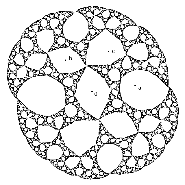
The fixed points are d , e , ¯e , and the other period threeorbit is a 7→b 7→c 7→a .Figure 3.Type C:Julia setfor themapz7→a + 1/(z2 −a2)witha ≈.7467 + .2286 i .Here the periodic critical orbit∞↔acaptures theorbit 0 7→b 7→c 7→−a 7→∞of the other critical point.19

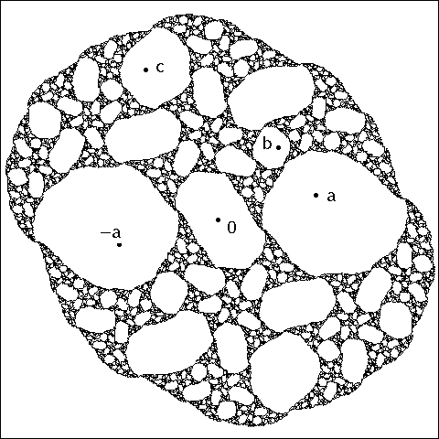
Figure 4.Type D: Julia setfor the mapz7→a + 1/(z2 −a2)witha ≈.8200 + .1446 i . (See [Bie].

)Here there are two disjoint periodic criticalorbits ∞↔a and 0 7→b 7→c 7→0 . This example is constructed by mating.of the Mandelbrot set.

Evidently, her construction yields many examples of quadratic rational maps withtwo distinct superattractive cycles. However, not every component of type D can be obtained in this way.Wittner has described a real quadratic map with attracting cycles of period 3 and 4 which cannot be obtainedby mating.

(Compare Appendix F.)20

Quadratic Mating Conjecture: It is conjectured that the mating fa ∐fb can be well defined asan element of Mcm2which depends continuously on a and b , whenever fa and fb do not belong tocomplex conjugate limbs of the Mandelbrot set M . (For this purpose, it is convenient to say that a map inM belongs to the t-limb if it either has a fixed point of multiplier e2πit , or is separated from the centralregion of M by the map which has such a fixed point, where t can be any angle in R/Z .

)One way of trying to construct such a mating can be described as follows.Let U(fa , ǫ) be theneighborhood of the filled Julia set K(fa) consisting of all points for which the Green’s function (canonicalpotential function) Ga of K(fa) takes values Ga(z) < ǫ . Let M = M(fa , fb , ǫ) be the compact Riemannsurface obtained from the disjoint union U(fa , ǫ)⊔U(fb , ǫ) by identifying the open subset U(fa , ǫ)∖K(fa)with U(fb , ǫ)∖K(fb) under the correspondence (G, t) ↔(ǫ −G, −t) , where G is the Green’s functionand t is the external angle.

By the Uniformization Theorem, M is conformally isomorphic to the RiemannsphereˆC .More explicitly, there is a unique conformal isomorphism which takes the critical points offa and fb to +1 and −1 respectively, and takes the point with coordinates G = ǫ/2 , t = 0 to thepoint at infinity inˆC . Now fa and fb fit together to yield a holomorphic map from M(fa , fb , ǫ) toM(fa , fb , 2ǫ) .

Identifying each of these manifolds withˆC . This yields a holomorphic map fromˆC toitself which has critical points at ±1 and a fixed point at infinity.

Thus it is a quadratic rational map ofthe form∐(fa , fb , ǫ) : w 7→(w + w−1 + c)/λ , where λ is the multiplier at infinity. (Compare (23)in Appendix C.) If the coefficients c and λ tend to well defined finite limits as ǫ →0 , then the limitingrational map may be called the matingfa ∐fb .

(For other, more standard, forms of the definition, see[Sh2], [Ta], [Bie]. )Common Fatou Boundary Points.

In the examples of Julia sets which are illustrated above, thereare many pairs of Fatou components which have a common boundary point, or (in Figure 2) even a Cantorset of common boundary points. However, this need not be the case.

Appendix F, written in collaborationwith Tan Lei, describes an example of a hyperbolic map for which no two Fatou components have a commonboundary point. The corresponding Julia set is a “Sierpinski carpet”.A Compactness Question.How can one decide whether some given hyperbolic component hascompact closure within the moduli space M2 ∼= C2 , or whether it is unbounded?

Any hyperbolic componentwith an attracting fixed point is certainly unbounded, and Figures 7, 9, 10, 16, 17 show many other examplesof unbounded components. On the other hand, consider a component obtained by mating two hyperboliccomponents of period ≥2 of the Mandelbrot set.

If the Quadratic Mating Conjecture is true, then it iseasy to show that such a component has compact closure, canonically homeomorphic to¯D × ¯D (at least inthe critically marked case). McMullen [Mc] has conjectured that whenever a degree d Julia set J(f) is aSierpinski carpet (Appendix F) the corresponding hyperbolic component in Md has compact closure.To conclude this section, we prove the following.Lemma 7.1.

If the Julia set of a hyperbolic map is connected, then it is locally connected.21

Proof outline (suggested by Douady). It suffices to consider the post-critically finite case.

For accord-ing to [Mc] every hyperbolic map with connected Julia set can be deformed through hyperbolic maps to apost-critically finite one, and according to [MSS] or [Ly] the topology of the Julia set, and the isotopy class ofits embedding into ˆC does not change under such a deformation. In the case of a periodic Fatou componentU , every internal ray from the super-attracting point lands at a well defined boundary point, which dependscontinuously on the initial angle.

(Compare the argument in [DH2, p. 24].) Since the continuous imageof a locally connected space is locally connected, it follows that the boundary of U is not only connectedbut also locally connected.

Since every Fatou component is eventually periodic ([Su]), it follows that: theboundary of every Fatou component is connected and locally connected. Let V ⊂ˆC be the complement ofthe post-critical set for f .

We will use the Poincar´e metric on V , and on its universal covering manifoldeV . Note that f −1 lifts to a well defined contracting map gf −1 on eV .

Each Fatou component U whichcontains no post-critical point lifts homeomorphically to a subset U ′ ⊂eV , and gf −1 maps U ′ to a set ofstrictly smaller diameter in the Poincar´e metric. In fact a straightforward compactness argument shows thatthe diameter shrinks by a factor bounded away from 1 .

For any ǫ > 0 , it follows that there are only finitelymany Fatou components of diameter > ǫ . From this, it follows easily that J is locally connected.

In fact,if two points of J are close to each other, then we can find a connected subset of J of small diametercontaining both points as follows. Draw a straight line segment between them, and replace its intersectionwith each Fatou component U with the entire boundary of Uif Uis small, or with a suitable smallconnected subset of ∂U otherwise.

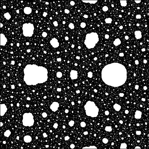
⊔⊓§8. The “Escape Locus”: Totally Disconnected Julia Sets.First a lemma above rational maps of arbitrary degree, to be proved in Appendix E.Lemma 8.1.

If all of the critical values of a rational map are contained in a single componentof the Fatou setˆC∖J , then the Julia set J is totally disconnected. Every orbit in the Fatouset converges either to an attracting fixed point, or to a parabolic fixed point of multiplicityprecisely equal to two.Here the multiplicity m ≥1 of a (finite) fixed point f(z0) = z0 is defined to be the degree of the firstnon-zero term in the Taylor expansion about z0 ,f(z) −z = α(z −z0)m + (higher terms) ,withα ̸= 0 .In the quadratic case, there is an explicit dichotomy, and an effective criterion.

See Yin [Y] and Makienko[Mak], as well as [Pr1], [R3].Lemma 8.2 The Julia set J of a quadratic rational map is either connected, or totally dis-connected and homeomorphic, with its dynamics, to the one-sided shift on two symbols. It istotally disconnected if and only if either:(a) both critical orbits converge to a common attracting fixed point, or(b) both critical orbits converge to a common fixed point of multiplicity two but neither criticalorbit actually lands on this point.The proof will be given at the end of this section.8.3.

Quadratic Examples. For the mapf(z) = z +2+z−1 ,one critical orbit 1 7→4 7→6.25 7→· · ·converges to the parabolic fixed point at infinity, while the other critical orbit −1 7→0 7→∞actuallylands at this fixed point.Thus the Julia set is connected.In fact J(f) is the interval [−∞, 0] .Forf(z) = ±(z + z−1) , both critical orbits±1 7→±2 7→±2.5 7→· · ·converge to the parabolic point atinfinity.

Since the multiplicity of the fixed point at infinity is either three (if the multiplier is +1 ) or one(if the multiplier is −1 ), the Julia set is again connected. It equals the imaginary axis plus the point atinfinity.

On the other hand, for z 7→z + c + z−1 with c > 2 , the Julia set is totally disconnected.8.4. Cubic Examples.

The situation for maps of higher degree is more complicated. The rationalmap z 7→2 + 2z3/(27(2 −z)) has connected Julia set, although the critical points 0, 0, 3, ∞are allcontained in an orbit 3 7→0 7→2 7→∞, which lands at a superattracting fixed point.

The polynomial map22

f(z) = z3 −12z + 12 has a Cantor set, contained in the interval [−4 , 3] , as Julia set, although the criticalpoint +2 belongs to this Julia set. The Julia set for the map z 7→536 (z −3)2(z + 4) is disconnected, butcontains the connected interval [0 , 5] .

For a thorough analysis of such polynomial examples, see [BH].The escape locus. There is just one hyperbolic component of type E in the moduli space M2 .

Wewill call it the hyperbolic escape locus, and denote it by E ⊂M2 . (Perhaps a better term would be “shiftlocus” or “totally disconnected locus” ?) If we work with critically marked conjugacy classes, there is a corre-spondinguniquecomponentEcm ⊂Mcm2.This escape component is very different from the other hyperbolic components.For amap f of type E, the Julia set J(f) is a Cantor set, and its complement is a connected open set of infiniteconnectivity.

Such a map can never be post-critically finite, so this hyperbolic component E does not haveany preferred center point.Here is a well known collection of examples. Consider the one-parameter family of quadratic polynomialsz 7→z2+c , which can be identified with the one-dimensional slice σ3 = 0 through the moduli space M2 .The intersection of this family with the escape locus E is precisely the complement of the Mandelbrot set.This complement is conformally isomorphic to C∖¯D , with free cyclic fundamental group.

The correspondingescape locus for polynomials of higher degree has been studied by Blanchard, Devaney and Keen, who showthat it has a very rich fundamental group.Using the critically marked moduli space, Rees shows that the escape locus Ecm has a rather compli-cated topology. In particular, her description implies that Ecm has the homotopy type of a Klein bottle,and hence has non-abelian fundamental group.

However, the unmarked escape locus E ⊂M2 has a muchsimpler description.Lemma 8.5. The hyperbolic escape locus E ⊂M2 is homeomorphic to the product D ×(C∖¯D) , where D is the open unit disk.More explicitly, if µ = µ(f) ∈D is the multiplier at the unique attracting fixed point of f , we willshow that the correspondence ⟨f⟩7→µ(f) yields a fibration of E over D , with fiber Eµ homeomorphicto C∖¯D (or equivalently to D∖{0} ).

As in 6.8, it will be convenient to work with the coordinates (µ, τ) ,where µ is the multiplier at the preferred (attracting) fixed point and τ is the product of the multipliersat the other two (repelling) fixed points. Thus each coordinate line µ = constant ∈D in the (µ, τ)-planecorresponds to a straight line Per1(µ) ⊂M2 , consisting of all conjugacy classes of maps which have anattracting fixed point of multiplier µ .

(Compare §3. These various straight lines Per1(µ) intersect eachother within M2 , but not within the escape locus, since for ⟨f⟩∈E the map f has only one attractingfixed point.

)The proof will be based on Goldberg and Keen [GK]. For each fixed µ ∈D , Goldberg and Keenshow that the complement Mµ of the escape locus in Per1(µ) ∼= C is canonically homeomorphic to theMandelbrot set M = M0 .

(This statement is quite likely true even in the limiting case µ = 1 ; compareFigure 5.) They prove this as an application of the theory of polynomial-like mappings (Douady and Hubbard[DH3]).

For ⟨f⟩∈Mµ the map f restricted to a suitable neighborhood of its Julia set is polynomial-likeof degree two with connected Julia set, and hence is hybrid-equivalent to a unique conjugacy class in M0 .Furthermore, by [DH3, §7] the resulting map from Sµ Mµ ⊂M2 to M0 is continuous.Caution: This statement is formulated rather differently in [GK], since the authors work with markedcritical points and hence study a 2-fold branched covering space Per1(µ)cm , which contains two disjointcopies of the Mandelbrot set for µ ̸= 0 . Note also that some notations (such as Rat2 ) which are used in[GK] are incompatible with the notations used here.It follows from the Riemann Mapping Theorem that the complementEµ = Per1(µ) ∩E ∼= C∖Mµis conformally isomorphic to the region C∖¯D .

In fact we can choose a canonical conformal isomorphismψµ : C∖¯D →C∖Mµ ,normalized so that the multiplier at infinity,λ(µ) = 1/ limz→∞ψ′µ(z)is real and positive. We mustshow that ψµ depends continuously on µ , using the topology of locally uniform convergence, so that the23

correspondence(µ , z) 7→(µ , ψµ(z)) ∈µ × Eµyields the required homeomorphism between D × (C∖¯D) and the escape locus E .Note that this multiplier λ(µ) provides an invariant measure of the “size” of the open set Eµ =ψµ(C∖¯D) . More generally, if U1 ⊂U2 are simply-connected neighborhoods of infinity in ˆC and if λ1 andλ2 are the multipliers at infinity of the corresponding Riemann maps C∖¯D →Ui , then it follows easilyfrom the Schwarz Lemma that λ1 ≤λ2 , with equality if and only if U1 = U2 .If this correspondence µ 7→ψµ were not continuous, then we could choose a sequence of points µi ∈Dconverging to a limit ˆµ ∈D so that the corresponding sequence of functions ψµi on C∖¯D did not convergelocally uniformly to ψˆµ .

However, since the ψµi belong to a normal family, we may assume after passingto a subsequence that these functions do converge locally uniformly to some univalent limitˆψ ̸= ψˆµ . It isnot hard to check that the image ˆψ(C∖¯D) must be a proper subset of the open set ψˆµ(C∖¯D) .

Therefore,as noted above, the multiplier ˆλ of ˆψ at infinity must be strictly less than the multiplier λ(ˆµ) of ψˆµ , sayˆλ < λ(ˆµ)/(1 + ǫ) with ǫ > 0 . Now the circle of radius 1 + ǫ in C∖¯D corresponds under ψˆµ to a loopwhich encloses a small neighborhood of the compact set Mˆµ .

For µi sufficiently close to ˆµ the compactset Mµi must be contained in this neighborhood, and it follows easily thatλ(µi) ≥λ(ˆµ)/(1 + ǫ) .Passing to the locally uniform limit as i →∞, since λ(µi) →ˆλ , we obtain a contradiction. ⊔⊓Remark 8.6: The escape locus incM2 .

If we work with the compactified moduli spacecM2 of§4, then the appropriate “hyperbolic escape locus” E∗⊂cM2 is a topological 4-cell with a preferred centerpoint, just like all other hyperbolic components. In fact, let E∗consist of E together with the 2-cellconsisting of all ideal points {µ , µ−1 , ∞} for which |µ| < 1 .

Then E∗fibers over the open disk withan open disk as fiber; and each fiber contains one and only one ideal point. By definition, the “center” ofthis filled in component is the ideal point ⟨0 , ∞, ∞⟩.

This center point can perhaps be identified with theimproper map ⟨z 7→z2 + ∞⟩, or with the limit of a sequence of quadratic maps “tending” to a constantmap.Next let us study the escape locus Ecm ⊂Mcm2, with marked critical points.We will prove thefollowing. (For a more precise description of Ecm , see [R3].

)Lemma 8.7.The critically marked escape locus Ecm contains a Klein bottle as retract.Hence the fundamental group of Ecm is non-abelian.This space Ecm can be described as a 2-fold branched covering of E , branched along the symmetrylocus S ∩E , which consists of all pairs (µ , τ) with µ ∈D∖{0} and τ = ( 2−µµ )2 . However, it seemssomewhat easier to take a different approach.

We will first work with fixed point markings, and describe thecorresponding escape locus Efm ⊂Mfm2. Recall that a point in Mfm2is specified by a 3-tuple (µ1 , µ2 , µ3)satisfying the cubic equation (1).

For a map in the escape locus, one of the three fixed points must beattracting and the other two must be repelling. Thus Efm actually splits into three distinct components,depending on which of the three marked fixed points is attracting.

To fix our ideas, suppose that |µ1| , |µ2| >1 > |µ3| . We will take the pair (µ1 , µ2) ∈(C∖¯D) × (C∖¯D) as independent parameters, solving for µ3by equation (2).

Of course not every such pair determines a map in the escape locus, or even a map with|µ3| < 1 . We first prove the following.Lemma 8.8.

If|µ1| > 6and|µ2| > 6 , then the associated map f belongs to the escapelocus.This estimate is probably far from sharp. (The largest |µ1| and |µ2| which I know, for f outside theescape locus, is given by µ1 = µ2 = −3 , for f(z) = −(z + z−1) .

)Proof of 8.8. We will use the normal formf(z) = z (z + µ1)µ2 z + 1=µ1 + zµ2 + z−124

of equation (3). (Compare Appendix C.) If |µ1| > 6 and |µ2| > 6 , then a brief computation shows thatf maps the annulus2/|µ2| < |z| < |µ1|/2into a compact subset of itself.

Furthermore, the polynomialµ2 z2 + 2z + µ1 , whose roots are the critical points of f , is strictly non-zero outside of this annulus, henceboth critical points are contained in the annulus. Using the Poincar´e metric for this annulus, we see thatboth critical orbits must converge to a common attracting fixed point.

The conclusion then follows by 8.2.⊔⊓Proof of 8.7. We can now easily construct a mapping from our preferred component of Efm to thetorus by the correspondence(µ1 , µ2) 7→(arg(µ1) , arg(µ2)) .The subset |µ1| = |µ2| = 7 maps homeomorphically to the torus, and hence is embedded in Efm as aretract.Now let us also mark the critical points, and hence pass to the 2-sheeted covering manifold Etm .

(Thesingle ramification point for the map Mtm2→Mfm2does not belong to the escape locus, and hence causes nodifficulty.) It is not difficult to show that a choice of critical point for f is equivalent to a choice of sign for±√1 −µ1µ2 .

(Compare the discussion following (22) in Appendix C.) Since the ratio (1 −µ1µ2)/(µ1µ2)always lies in the left half-plane when |µ1µ2| > 1 , this is equivalent to making a choice of sign for thegeometric mean η = ±√µ1µ2 . In other words, our component of Etm can be identified with an opensubset of the manifold consisting of all (µ1 , µ2 , η) ∈(C∖¯D)3 for which η2 = µ1µ2 .

In particular, weobtain an explicit retraction onto the torus consisting of all(µ1 , µ2 , η) ∈C3for which|µ1| = |µ2| = |η| = 7andη2 = µ1µ2 . (16)In order to obtain the hyperbolic component Ecm , as described by Rees, we must pass to a quotient spaceby identifying under the involution of Etm which interchanges the role of the two repelling fixed points.

Abrief computation shows that this corresponds to the fixed point free involution(µ1 , µ2 , η) ↔(µ2 , µ1 , −η) .The quotient space Ecm is still a smooth manifold. If we collapse the torus (18) under this involution, weobtain a Klein bottle.

Thus this argument proves that Ecm contains a Klein bottle as retract, and hencethat π1(Ecm) retracts onto the fundamental group of a Klein bottle. ⊔⊓(If we try to carry out the same argument for the unmarked escape locus E ⊂M2 , then we mustsimply work with the torus |µ1| = |µ2| = 7 and the orientation reversing involution (µ1 , µ2) 7→(µ2 , µ1) .In this case, the quotient space is a M¨obius band, which has the homotopy type of a circle.

Thus we couldconclude only that E contains a circle as retract. )25

Recall that Mcm2has the homotopy type of a 2-sphere.It is conjectured that the inclusion mapEcm →Mcm2is homologically non-trivial, or more explicitly that it induces an isomorphism of 2-dimensionalhomology with mod 2 coefficients.Proof of 8.2. To conclude this section, let us prove that every quadratic Julia set is either connectedor totally disconnected.

Note that J is connected if and only if every component of the Fatou setˆC∖Jis simply-connected. According to Sullivan, every component ofˆC∖Jis eventually periodic, and everyperiodic component is either a Siegel disk, a Herman ring, or an immediate basin for some attracting orparabolic point.

According to Shishikura [Sh1], there are no Herman rings in the quadratic case. We willmake frequent use of the fact the a ramified covering of a simply-connected region which has only oneramification point must again be simply-connected.First suppose that every periodic Fatou component is simply-connected.

Any cycle of Fatou componentsmust either contain a critical point (in the attracting or parabolic cases), or have a critical orbit which isdense in its boundary (in the Siegel case). Thus there is at most one critical point left over.

It followsinductively that every Fatou component is simply-connected.Now suppose that some periodic Fatou component is not simply-connected.Evidently it must bean immediate basin for some attracting or parabolic periodic point.Such an immediate basin can bereconstructed from a simply-connected neighborhood of the fixed point in the attracting case, or froma simply-connected petal in the parabolic case, by taking a direct limit of successive ramified coverings,ramified only at the critical values. The result will again be simply-connected, unless both critical pointsbelong to the same connected component.

But in that case, it follows from Lemma 8.1 that J(f) is totallydisconnected. (Compare [R3] and Appendix E.)If both critical orbits converge to the same attracting or multiplicity two fixed point, then at least onecritical point must belong to the immediate basin U .

Hence the map f restricted to U is two-to-one.Since f is quadratic, and since U is fixed under f , this implies that U is fully invariant: U = f −1(U) .Hence both critical points belong to U , and again we can apply 8.1.Finally, we must prove that a totally disconnected J is homeomorphic to a one-sided two-shift. In thehyperbolic case, this is proved in [GK].

The key step is the construction of an embedded disk ∆which con-tainsbothcriticalvaluesandisforwardinvariant,f(∆) ⊂∆. The two components of ˆC∖f −1(∆) then cover the Julia set, and form the required Bernoullipartition.

In the parabolic case, we modify this argument by constructing a simply connected open petal Pwhich contains both critical values and satisfies f(P) ⊂P . Again the two components of ˆC∖f −1(P) coverthe Julia set and form the required Bernoulli partition.

The proof that a point in the Julia set is uniquelydetermined by its symbol sequence with respect to this partition is now more delicate. However, since acompletely analogous argument is carried out in Appendix E, details will be left to the reader.

⊔⊓26

§9. Complex 1-Dimensional Slices.The moduli space M2 can be thought of as a kind of table of contents, with each point ⟨f⟩∈M2corresponding to a different form of dynamic behavior.

Since this space is a complex 2-manifold, it is difficultto visualize all of it it directly. Hence it may be helpful to try to describe what kinds of behavior occur for⟨f⟩belonging to some 1-dimensional slice through M .As a first example of a dynamically interesting 1-dimensional slice, suppose that we choose some fixedinteger n ≥1 and some fixed complex number µ and consider the curve Pern(µ) ⊂M2 consisting of allconjugacy classes of maps which possess a periodic point of period n and multiplier µ .

(See 3.4, 4.2.) Thecase µ = 0 is of particular interest.

(Compare [R4], [R5], [M3], [M5], and see Figures 7, 9.) Evidently thecenter point of every hyperbolic component must belong to at least one of these curves Pern(0) .

For anyµ in the closed disk |µ| ≤1 , the fact that ⟨f⟩belongs to Pern(µ) imposes very strong restrictions on thedynamics of f . The cases where µ is a root of unity are noteworthy, since these curves contain faces wheretwo or more hyperbolic components of M2 come together along a common boundary.

(Figures 5, 6, 8. )We can also consider curves for which one critical orbit is eventually periodic, say f ◦t(ω1) = f ◦t+n(ω1) .See Figure 11 for the case t = 2 , n = 1 .

These curves also contain common boundary faces between twodifferent hyperbolic components. The symmetry locus of §5 is another curve of interest.

(Figure 12. )As a final interesting family of curves, for each integer t ≥1 we can consider all f such that the t-thforward image of one critical point is equal to the other critical point, f ◦t(ω1) = ω2 .

See Figure 13 for thecase t = 1 . Note that the center point of every hyperbolic component of type B or C must belong to atleast one of these curves.Here is a more detailed discussion of some sample curves.Figure 5.

The bifurcation locus in Per1(1) seems to be a homeomorphic copy ofthe Mandelbrot set boundary, with the cusp point straightened out. Here Per1(1)is represented as the −a2-plane for the family of maps fa(z) = z + a + 1/z , havinga double fixed point of multiplier +1 at infinity, and having critical points at ±1 .

(Compare Appendix C.) The other fixed point has multiplier 1 −a2 , and the period2 orbit has multiplier 9 −4a2 . Curves of the formRe(f ◦na (±1)/a) −n = constantfor large n are also shown.Period 1.

As noted in 3.4, the curves Per1(µ) are particularly easy to describe: Each locus Per1(µ)is a straight line of slope µ + µ−1 in the (σ1 , σ2)-coordinate plane, given for example by the equationPer1(µ) :µ3 −σ1 µ2 + σ2 µ + 2 −σ1 = 0 .First consider the case µ = 0 . Putting the fixed critical point at infinity, we can use the normal form27

Figure 6. The bifurcation locus in Per1(−1) = Per2(1) is a distorted copy of the Man-delbrot set boundary with the 1/2-limb missing (collapsed to the point at infinity).This picture shows part of the −a2-plane for the family of maps z 7→−(z + a + z−1) ,having a fixed point of multiplier −1 .

The notation p/q indicates that the map alsohas a fixed point of multiplier e2πip/q . (The case p/q = 1/2 would correspond to thepoint at infinity.

)Figure 7. Bifurcation locus in Per2(0) (part of the −a3-plane for the family of mapsz 7→a/z + 1/z2 , with a critical point of period 2 at z = 0 ).

This appears to bea homeomorphic copy of Figure 6.The types of some of the more conspicuoushyperbolic components are indicated.28

z 7→z2 + c . (Here σ1 = 2 and σ2 = 4c .) The corresponding bifurcation locus1 in the c-plane is theboundary of the familiar Mandelbrot set.

The hyperbolic components which intersect Per1(0) all have typeD or E. (Remark: If we lift to the critically marked moduli space Mcm2, then the locus Per1(0) lifts toa union of two lines which intersect transversally. In fact, using coordinates A, B, C as in 6.1, the locusPercm1 (µ) splits as the union of a line A = B = 0 for which the first critical point is fixed and a lineA = C = 0 for which the second critical point is fixed.

These two lines intersect transversally at the pointA = B = C = 0 , corresponding to the map z 7→z2 with both critical points fixed. )As noted in the proof of 8.5, the bifurcation locus in the line Per1(µ) varies by a continuous isotopy asµ varies within the open unit disk.

As shown in Figure 5, it even seems to retain the same topology as µtends non-tangentially to +1 . On the other hand, as µ →−1 non-tangentially, the central region of theMandelbrot set opens out so as to contain a full half-plane, and the entire 1/2-limb of the Mandelbrot setdisappears to infinity.

Also, a number of the tentacles of the Mandelbrot set join together, so as to enclosenew regions. Compare Figure 6.Figure 8.

Bifurcation locus in Per1(e2πi/3) . Here the 2/3-limb of the Mandelbrotset has disappeared to infinity.

Again various tentacles of the Mandelbrot set havecome together to enclose new regions. Under a slight perturbation, the fixed point ofmultiplier e2πi/3 will become repelling but split offan attracting period three orbit,yielding hyperbolic components of type B, C, and D, as indicated.

(This picture looksrather different from Figure 6 since a different algorithm was used.) The intersectionpoint of this line with the line Per2(−3) of Figure 10 is indicated by a heavy dot(upper right).Similarly, as µ tends to e−2πip/q non-tangentially, the entire p/q-limb disappears to infinity.

The casep/q = 2/3 is illustrated in Figure 8. This disappearance is one aspect of Tan Lei’s observation that matingbetween two quadratic polynomials is never possible when the two belong to complex conjugate limbs of theMandelbrot set.1 By the bifurcation locus for a parametrized family of maps {fa} we mean the closed set consisting ofparameter values a for which the associated Julia set J(fa) does not vary continuously under deformationof a .

Compare [MSS], [Ly].29

A more precise statement has recently been given by Petersen [Pe]. If f ∈Rat2 has an attractingfixed point of multiplier µ = µ1 and a repelling fixed point with combinatorial rotation number p/q andmultiplier µ2 , then Petersen shows that a suitable choice of log(µ2) is contained in the disk which istangent to the imaginary axis at 2πip/q , and which contains log(1/µ1) as boundary point.

Hence, as µ1tends to e−2πip/q non-tangentially, it follows that µ2 tends to e2πip/q . If 0 < p/q < 1 , then it followsfrom (2) that the multiplier µ3 at the third fixed point tends to infinity.

Thus, the entire p/q-limb of theMandelbrot set must be missing in the locus Per1(e−2πip/q) .Period 2. According to Lemma 3.6, the curve Per2(µ) is also a straight line in the (σ1 , σ2)-coordinateplane, given by the equation 2σ1 + σ2 = µ .

For µ = +1 , this locus Per2(1) coincides with the locusPer1(−1) of Figure 6. As µ varies from +1 to zero, the right hand region of Figure 6 opens up evenfurther, as shown in Figure 7.

There is some difficulty in finding a good normal form in the case µ = 0 ,since the curve Per2(0) includes the special point ⟨z 7→1/z2⟩, which has an anomalously large group ofautomorphisms. If we place the period 2 critical point at the origin with its image at infinity, and normalizeby an appropriate scale change, then we get the formulaf(z) = az + 1z2 .This normal form is not unique, since for any cube root of unity λ the map f(λ z)/λ will have the sameform, but with the parameter a replaced by λ a .

Thus to obtain an invariant we must pass to a3 , whichranges over C . In fact it turns out that a3 −6 = σ1 .Figure 9.

Picture in Per3(0) , showing the log(c)-plane for the family of mapsz 7→1 −(1 + c)/z + c/z2with a critical point of period 3 at z = 0 . (The top and bottom are to be identified,with a little bit of overlap.) There are only two components of type B in the cylin-der C/2πiZ , but many components of type C and D. For the three most prominentcomponents of type D, corresponding to the three period 3 components in the Man-delbrot set, internal angles have been indicated.

Note that the internal angles 1/3respectively 2/3 respectively 1/2 correspond to points at infinity.30

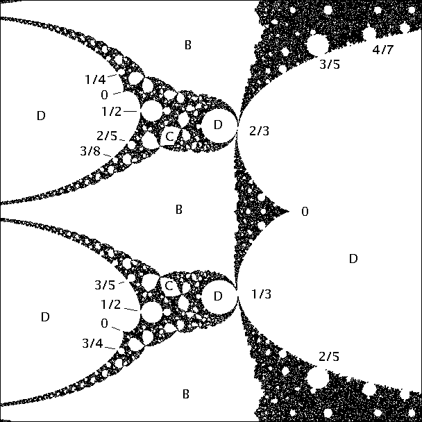
Period 3. The curve Per3(0) also has genus zero, being conformally isomorphic to a punctured planeor cylinder.

We may put the periodic critical point at the origin, with orbit 0 7→∞7→1 7→0 . This yieldsthe unique normal formz7→1 −1 + cz+cz2,where now the parameter c ranges over C∖{0} .

Compare Figure 9, which shows the log(c)-plane. Thelower left hand portion of this picture can be understood as a perturbation of Figure 8, and similarly theupper left portion can be understood as a perturbation of a complex conjugate figure.

In fact, as µ variesfrom 0 to 1 −ǫ the bifurcation locus in Per3(µ) varies continuously. However, in the limiting case asµ →1 the locus Per1(µ) degenerates into a union of three straight lines.

(Compare 4.3.) Two of theselines correspond to the locus Per1(e2πi/3) and its complex conjugate, while the third line can be identifiedwith the locus Per2(−3) .

Thus, in order to understand the right half of Figure 9, we must also studythe bifurcation locus in Per2(−3) , as shown in Figure 10. Unfortunately, it seems to require considerableimagination to see how to cut and paste Figure 8, its complex conjugate, and Figure 10 so as to obtainFigure 9.For more detailed studies of the curve Per3(0) and of the associated dynamics, see [R4], [R5], [W].Figure 10.Bifurcation locus in the linePer2(−3) , which coincides with the lo-cus of⟨f⟩for whichfhas a non-degenerate orbit of period3 and multiplier+1 .

(Caution: The algorithm used to draw this Figure is not too satisfactory.In fact, the boundary of the outer region looks rather ragged because of very slowconvergence. )Period 4.

The curve Per4(0) is isomorphic to a three times punctured plane. Again we place the peri-odiccriticalpointattheorigin,andnowsupposethatithasorbit0 7→∞7→1 7→ρ 7→0 .Here the parameter ρ can be described as the cross-ratio of the points inthis orbit.

It is not difficult to check that this invariant ρ determines the quadratic map uniquely, andthat ρ ranges over the set C∖{0 , 1/2 , 1} . The value 1/2 is excluded since as ρ →1/2 the associatedquadratic map degenerates to a fractional linear map z 7→1 −(2z)−1 , and the class ⟨f⟩tends to the idealpoint {i , −i , ∞} .31

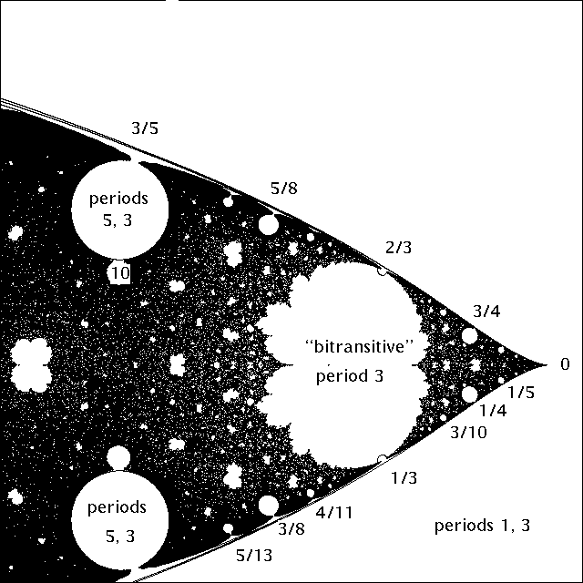
Figure 11. Picture for the λ-plane for the family of maps z 7→λ(z + 2 + z−1) withpre-periodic critical orbit −1 7→0 7→∞7→∞.

In the more prominent regions with anattracting orbit, the period is indicated.Pre-periodic critical orbits. Another important class of parameter slices are those for which onecritical point is pre-periodic.

Since a non-periodic critical point cannot map directly to a periodic pointwhen the degree is 2, the simplest possibility is that the second forward image f ◦2(ω1) is fixed. If we placethe critical points at ±1 and this fixed point at infinity, this leads to the normal formw 7→λ (w + 2 + w−1) ,with −1 7→0 7→∞.

Note that λ−1 is the multiplier of the fixed point at infinity. A corresponding picturein the λ-plane is shown in Figure 11.

Here values of λ outside of the unit disk correspond to maps in theescape locus E . However points within the unit disk correspond to non-hyperbolic maps, since one criticalorbit lands on a repelling fixed point.Maps with J = ˆC .

All of our previous curves have included only maps with at least one attracting orparabolic orbit. Hence the associated Julia set has always been a proper subset of the Riemann sphere.

How-ever,amapinthepresentfamily{w 7→λ(w+2+w−1} need not have any attracting or parabolic fixed point. In fact the orbits of both criticalpoints ±1 may eventually land on repelling cycles.

This happens for example for the value λ0 = −1/4 , with1 7→−1 7→0 7→∞. The Julia set for such a map is necessarily the entire sphere.

In fact, as an immediateconsequence of a Theorem of Rees [R2] we have the following much sharper statement: Every neighborhoodof such a point λ0 contains a set of parameter values λ of positive area (2-dimensional Lebesgue measure)for which the associated Julia set is the entire Riemann sphere ˆC .32

Figure 12. Picture of the symmetry locus S , represented as the k-plane for thefamily of maps z 7→k (z + z−1) .

The component of type D on the right is centered atk = 1/2 , with both critical points fixed, while the component of type B on the left iscentered at k = −1/2 , with critical points −1 ↔1 .The symmetry locus. An apparently quite different example is provided by the branch locus orsymmetry locus, consisting of all conjugacy classes ⟨f⟩for which f has a non-trivial automorphism.

ByLemma 5.1 this locus can be described parametrically as the set of ⟨fk⟩withfk(z) = k (z + z−1) ,wheretheparameterkrangesoverC∖{0} .Apictureofthek-planeisshowninFigure12.(Compare[HP]. )Notethatthisfigureiscentrallysymmetric.Infact,sincefk(−z) = −fk(z) = f−k(z) it follows that fk ◦fk = f−k ◦f−k .Hence the Julia set J(fk) is pre-cisely equal to J(f−k) , and the bifurcation diagram in the k-plane, describing different forms of dynamicalbehavior, is essentially invariant under the involution k 7→−k .

This does not mean that fk has preciselythe same dynamics as f−k . For example f1 has a triple fixed point while f−1 has three distinct fixedpoints.) As in the previous example, this symmetry locus contains maps like z 7→i(z + z−1)/2 for whichboth critical orbits eventually land on repelling cycles (±1 7→±i 7→0 7→∞) .C.

Petersen has pointed out to me that this family of maps is closely related to the locus of Figure 11.In fact the two-to-one substitution w = z2 semi-conjugates the family z 7→k (z + z−1) to the familyw 7→k (√w + √w−1)2 = λ(w + 2 + w−1) ,withλ=k2 .Notethatsymmetricpairsofhyperboliccomponentsinthek-planeofFigure12correspondto“sub-hyperboliccomponents”,whereonlyonecriticalorbitconverges to a periodic attractor, in the λ-plane of Figure 11.33

Figure 13.a3-plane for the family of maps z 7→a + 1/z2 , with one critical pointmapping directly to the other. In the more conspicuous hyperbolic components (typeB or E), the period of the attractor is indicated.Maps for which one critical point maps eventually to the other.

The simplest possibility hereis that one critical point maps directly to the other. Taking the critical points to be 0 →∞, we obtain thenormal form z 7→a + 1/z2 of Figure 13.As in the previous two examples, this family contains maps for which the critical orbits eventually landon a repelling cycle.

This happens for example if f(z) = a + 1/z2 with a3 = −0.5 , so that 0 7→∞7→a 7→−a 7→−a . Again, it follows from [R2] that there is a set of parameter values of positive area for which theassociated Julia set is the entire Riemann sphere.34

§10. Real Quadratic Maps.Consider a quadratic rational map which has real coefficients, and hence induces a map from the circleR ∪∞into itself.

We will distinguish seven different cases, depending on the topology of this map from thecircle to itself.First suppose that the two critical points of f are conjugate complex, then it is easy to check that finduces a two-to-one covering map from R ∪∞onto itself. In this case, we must must distinguish betweenthe positive derivative case, where f maps this circle with degree +2 , and the negative derivative casewith degree −2 .On the other hand, suppose that the two critical points are both real.

Then f maps the entire circleR ∪∞onto a closed interval I = f(R ∪∞) which is bounded by the two critical values. Evidently, inorder to study both critical orbits, we need only study the dynamics of f restricted to this interval I .Definition.

We will say that a real quadratic map with real critical points is either monotone orunimodal or bimodal according as the interior of this interval I = f(R ∪∞) contains either no criticalpoints, one critical point, or both critical points.In the monotone case, we must distinguish betweenmonotone increasing and monotone decreasing. Similarly, in the bimodal case we distinguish between (+ −+)-bimodal and (−+ −)-bimodal according to the pattern of increasing and decreasing laps.The unimodal case is illustrated in Figure 14, where just one critical point ω1 = 0 belongs to theinterior of the interval I = [−1 , 1] .

(Since the other critical point ω2 = 1 belongs to the boundary ofI , we see that this particular map lies on the boundary between the unimodal and the (+ −+)-bimodalregions of the “real moduli space”. )-101Figure 14.

Graph of a borderline “unimodal” real quadratic mapf0(x) = (1 −2x −x2)/(1 −2x + 3x2)with f0(R ∪∞) = [−1 , 1] . In this example, both critical orbits land on the repellingfixed point 1/3 , hence the (complex) Julia set J(f0) is the entire Riemann sphere.It is not difficult to check that a conjugacy class ⟨f⟩∈M2possesses a representative with realcoefficients if and only if the two invariants σ1 and σ2 of §3 are both real.

Hence we define the realmoduli space to be simply the real (σ1 , σ2)-plane. In general, the real representative for ⟨f⟩∈M2 isunique up to real conjugacy.

However, in the special case where ⟨f⟩belongs to the real part of the symmetrylocus S of §5 this is not true. In fact, for the conjugacy class of f(x) = λ (x + x−1) where λ ∈R∖{0} , wecan choose f itself as real representative, with critical points ±1 and degree zero.

But we can also takef(ix)/i = λ(x −x−1) as representative, with critical points ±i and with degree equal to 2 sgn(λ) .The classification of real quadratic maps into seven different topological types corresponds to a partitionof real moduli space into seven different regions, as indicated in Figure 15. More precisely, the real (σ1 , σ2)-plane is cut up into seven pieces by the two real branches of the symmetry locus S , and by the vertical linesσ1 = 2 and σ1 = −6 which correspond to the classes ⟨f⟩for which f(ω1) = ω1 respectively f(ω1) = ω2 .35

z21/z2z2 - 2-62012-8unimodal+ - +bimodaldegree +2monotone+z+z-1- + -bimodaldeg-2monotonef(ω ) = ω21f(ω ) = ω11-SSFigure 15. Rectangle [−12, 10×[−10, 22] in the real (σ1 , σ2)-plane, showing the sevenregions corresponding to different topological descriptions of f on R ∪∞.

(Drawnto the same scale as Figures 1 and 16.) These seven regions are bounded by thesymmetry locus S together with the vertical lines σ1 = −6 and σ1 = 2 .

The lociPer1(±1) have been drawn in as dotted lines.The bifurcation locus in the real (σ1 , σ2)-plane is plotted in Figures 16 and 17. Figure 16 shows thesame region as Figures 1 and 15.

Note that the vertical line σ1 = 2 parametrizes the family of real quadraticpolynomials x 7→x2 + constant , while the line σ1 = −6 parametrizes the family of maps which carry onecritical point to the other — that is, the real axis of Figure 13. As in Figure 13, the numbers label hyperboliccomponents of type B, with attracting period as indicated.

Figure 17 shows a much larger region, so thatwe can begin to see the limiting behavior as (σ1 , σ2) tends to the line at infinity Per1(∞) .Significant features of both Figures are the following. The two straight lines Per1(1) of slope +2 andPer1(−1) of slope −2 cut the plane into four quadrants:Top quadrant.

This is part of the escape locus. If we restrict attention to maps in this quadrantwith two real critical points, then the real dynamics is completely trivial: the successive images of R ∪∞converge uniformly to the real fixed point.Right hand quadrant.

These are the maps with two attracting fixed points. They form the real partof the hyperbolic component D1,1 consisting of all maps with two attracting fixed points.

It is centered atthe point ⟨z 7→z2⟩.Bottom quadrant. As we pass from the right hand quadrant to the bottom quadrant, one fixed pointbifurcates to a period two orbit, then to period four, and so on, in the usual Sharkovskii pattern, until weagain reach the escape locus.

(Note in fact that the standard quadratic polynomial family is just the sectionof this picture with the vertical line σ1 = 2 .) However, this lower component of the real escape locus hasmuch more complicated real dynamics, since the entire Julia Cantor set is contained in R ∪∞.Left hand quadrant.

Here we evidently have a much more complicated situation. There are con-spicuous hyperbolic components of type B, bordered by hyperbolic components of type C. There are alsohyperbolic components of type D, at least within the bimodal region σ1 < −6 (compare Appendix F), butthese are very tiny, and are not visible in the pictures.

For σ1 very negative, with σ2/σ1 ≈2 cos(2πip/q)we are in a component of type B with attracting orbit of period q . Some representative values of p/q areindicated along the left margin.

For p = 1 note that these are exactly the same as the components which36

Figure 16. Picture of the rectangle [−12, 10]×[−10, 22] in the real (σ1 , σ2)-plane, em-phasizing dynamic behavior.

(Horizontal scale exaggerated.) The periods of (possiblycomplex) attracting orbits for some of the more prominent hyperbolic componentsare indicated.

As we traverse any vertical line with −6 ≤σ1 ≤2 , we follow a fullfamily of unimodal maps. For maps within the top component of the escape locus,there are no real periodic orbits other than the attracting fixed point.

However, formaps in the bottom component, the entire Julia set is real.occur in Figure 13. In fact, the real axis in Figure 13 corresponds exactly to the vertical line σ1 = −6 inFigures 16, 17.The real topological classification of Figure 15 can be compared with the complex dynamic classificationof Figures 16, 17 as follows.Monotone case: If fis +monotone, clearly the two critical orbits must converge, either to a singlefixed point or to two distinct fixed points.

If neither fixed point is parabolic, this means that ⟨f⟩mustbelong either to the hyperbolic component of type D1,1 with two attracting fixed points, or to the escapecomponent E . Similarly, in the −monotone case the two critical orbits must converge to a common fixedpoint or period two orbit.

In the non-parabolic case, this means that ⟨f⟩belongs either to the escapecomponent or to the period two hyperbolic component of type B .Unimodalcase:Herethereisawiderangeofpossibledynamicbehavior.Inthehyperbolic case, ⟨f⟩may belong to a component of any one of the four types B, C, D, or E. One essentialrestriction is that there cannot be two attracting orbits of period greater than one.Bimodal case: Not all bimodal maps can arise as quadratic maps, since the condition that each point hasat most two pre-images imposes an essential restriction. In particular, the topological entropy of the mapI →I can be at most log 2 .

In the (−+ −) case, there is another quite strong restriction:Lemma 10.1. Every (−+ −)-bimodal quadratic map must have an attracting fixed point.Proof.

Clearly such a map must have three fixed points on the interval I = f(R∪∞) , and two of the threemust have negative multipliers, say µ1 , µ3 < 0 . If these two fixed points were both repelling or parabolic,µ1 , µ3 ≤−1 , then the formula µ2 = (2 −µ1 −µ3)/(1 −µ1µ3) would imply that the third fixed point alsohad negative (or infinite) multiplier, which is impossible.

⊔⊓37

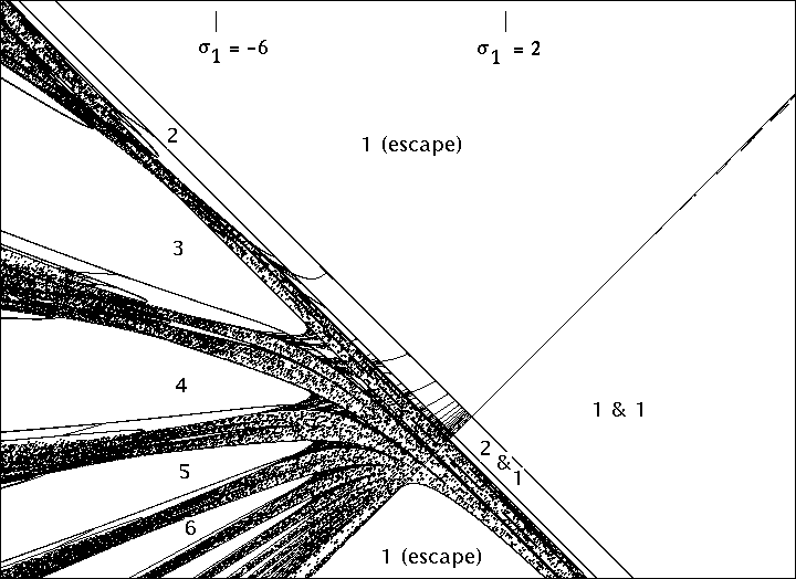
Figure 17. Picture of the much larger rectangle [−25, 10]×[−55, 55] in the real (σ1 , σ2)-plane.

For σ1 very negative, with σ2/σ1 ≈2 cos(2πip/q) we are in a component oftype B with attracting orbit of period q . Some representative values of p/q areindicated along the left margin.Degree ±2 case: Here the dynamics is again sharply restricted.Lemma 10.2.

If the real quadratic map f has complex conjugate critical points, so that itinduces a covering mapping of degree ±2 from the circle R∪∞onto itself, then the (complex)Julia set J(f) is either the circle R ∪∞, or a Cantor set contained in R ∪∞. Both criticalorbits converge to attracting orbits of period ≤2 , or to a parabolic fixed point.The proof is not difficult, and will be omitted.

⊔⊓38

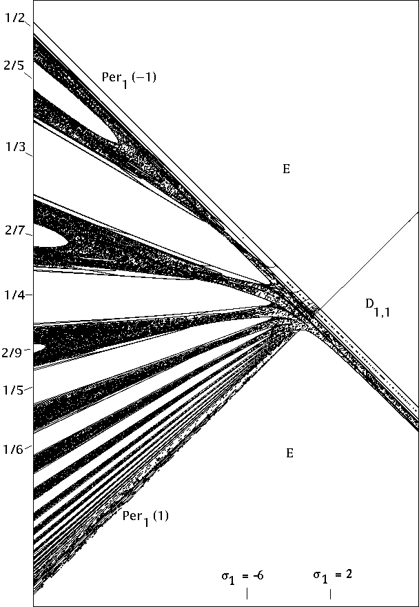
Appendix A. Resultant and Discriminant.This will be a brief summary of standard material.

Proofs may be found, for example, in [vW]. Fix twointegers m , n ≥0 .

Let p range over the vector space Vm consisting of all complex polynomial functionsp(z) = a0 zm + · · · + amof degree ≤m , and let q range over the space Vn of polynomialsq(z) = b0 zn + · · · + bnof degree ≤n . The resultant resultm,n(p, q) , can be characterized as the unique function from Vm × Vnto C which is bimultiplicativeresultm1+m2,n(p1 · p2 , q) = resultm1,n(p1 , q) · resultm2,n(p2 , q)resultm,n1+n2(p , q1 · q2) = resultm,n1(p , q1) · resultm,n2(p , q2)and which coincides with the determinant in the degree 1 , 1 caseresult1,1(az + b , cz + d) = ad −bc .This function is (−1)mn-symmetric and bihomogeneous of degree (n, m) , that isresultm,n(p, q) = (−1)mn resultn,m(q, p)resultm,n(λp , µq) = λnµm resultm,n(p, q) .Note that the subscripts m, n are essential, since we sometimes consider polynomials with leading coefficientzero.

However, in practice we will suppress these subscripts whenever they are clear from the context. Theresultant can be expressed as an (m + n) × (m + n) determinant, for exampleresult(az2 + bz + c , pz2 + qz + r) = detabc00abcpqr00pqr.In the special case m = 0 note that result(a0 , q) = an0 is completely independent of q , while for m = 1 ,if p(z) = z −ξ thenresult(z −ξ , q) = q(ξ) .

More generally, whenever the leading coefficient a0 isnon-zero, we can factor p asp(z) = a0 (z −ξ1) · · · (z −ξm) , and it follows thatresult(p, q) = an0mY1q(ξi) . (Ontheotherhand,ifa0=0 ,thenresultm,n(p, q)=(−1)n b0 resultm−1,n(p, q) .

)Similarly, if b0 ̸= 0 then we can set q(z) = b0 (z −η1) · · · (z −ηn) and writeresult(p, q) = (−1)mn bm0nY1p(ηj) = an0 bm0mY1nY1(ξi −ηj) .The resultant may well be non-zero even if one of the leading coefficients is zero. However, if both a0 = 0and b0 = 0 so that deg(p) < m and deg(q) < n , then resultm,n(p, q) = 0 .39

In fact the resultant resultm,n(p, q) is zero if and only if either:(1) the two polynomials p and q have a root in common, or(2) both deg(p) < m and deg(q) < n .Closely related is the discriminant of a polynomial of degree m or less. This is a polynomial functiondiscrm : Vm →C , which is homogeneous of degree 2m −2 ,discrm(λp) = λ2m−2 discr(p) .If the leading coefficient a0 is non-zero, the discriminant can be defined by the formuladiscrm(p) = (−1)m(m−1)/2 resultm,m−1(p, p′)/a0 ,where p′ is the derivative.

Alternatively, settingp(z) = a0 (z −ξ1) · · · (z −ξm) , it can be defined by theformuladiscr(p) = a2m−20Yi

On the other hand, if a0 = 0then discrm(p) = a21 discrm−1(p) . In particular, for any m ≥2 , if both of the leading coefficients a0and a1 are zero, then the discriminant discrm(p) is zero.

Here are explicit formulas, for the cases m ≤3which will be of interest.discr1(az + b) = 1 ,discr2(az2 + bz + c) = b2 −4ac ,discr3(az3 + bz2 + cz + d) = b2c2 −4ac3 −4b3d −27a2d2 + 18abcd . (17)Appendix B.

The Space Ratd of Degree d Rational Maps.This appendix will describe results from Segal [Se], as well as some consequences of his work. For eachinteger d ≥0 we can form the space Ratd consisting of all rational maps f(z) = p(z)/q(z) wherep(z) = a0 zd + · · · + adandq(z) = b0 zd + · · · + b0(18)are complex polynomials with no common root, and with leading coefficients a0 and b0 which are not bothzero.

Evidently Ratd is a Zariski open subset of the complex projective space CP2d+1 consisting of ratios(a0 : . .

. : ad : b0 : .

. .

: bd) . We will write such ratios briefly as (p : q) ∈CP2d+1 .

More explicitly, this openset can be described as the complementRatd ∼= CP2d+1∖WdwhereWdisthealgebraicvarietyconsistingofallratios(p:q)whoseresultantresult(p, q) = resultd,d(p, q)is equal to zero. (See Appendix A.) In particular, it follows easily that Ratdis a smooth connected complex manifold of complex dimension 2d + 1 .If we map each rational map f ∈Ratd to the image f(∞) = a0/b0 in the Riemann sphere S2 = C∪∞,then we obtain a fibrationRat0d ֒→Ratd →→S2where Rat0d is the fiber, consisting of rational maps which fix the point at infinity in S2 .

Definition. LetMapd be the infinite dimensional space consisting of all continuous maps from S2 to itself of degree d ,and let Map0d be the subspace consisting of maps which fix some base point.

Then according to Segal [Se]:Assertion B.1. The inclusions Ratd ⊂Mapd and Rat0d ⊂Map0d induce homotopy equiva-lences through dimension d .As model for the fiber Rat0d , Segal uses the space of rational maps f(z) = p(z)/q(z) where p and qare monic polynomials of degree d , so that f(∞) = +1 .

With this normalization, using an argument dueto J. D. S. Jones, he proves the following.40

Assertion B.2. For d ≥1 the fundamental group π1(Rat0d) is free cyclic.

In fact let (p, q)range over pairs of monic degree d polynomials with no common root. Then the correspondencep/q 7→result(p, q) ∈C∖{0}defines a fibrationRat0d →C∖{0} ,(19)which induces an isomorphism of fundamental groups.The fiber Fd of this fibration consists of all pairs (p, q) of monic degree d polynomials which haveresultant result(p, q) equal to 1 .

Thus Fd can be considered as an algebraic hypersurface in the coordinatespace C2d . As an immediate consequence:Corollary.This fiber Fdis simply connected.Furthermore, the universal covering spacegRat0d is homeomorphic to Fd × C .Developing these ideas further, we have the following statement.

LetEd = {(p, q) : result(p, q) = 1}be the affine hypersurface in C2d+2 consisting of all pairs of polynomials (p, q) of the form (18) whichhave resultant result(p, q) equal to 1 . Note that there is a natural fibrationFd ֒→Ed →→C2∖{(0, 0)} ,(20)where the projection map from Ed to C2∖{(0, 0)} carries each pair (p, q) of polynomials with resultant1 to the pair (a0 , b0) of leading coefficients.

In fact each matrixabcdin the group SL(2, C) actson the total space Ed , carrying each (p, q) with resultant 1 to (ap + bq , cp + dq) . Using the fact thatSL(2, C) is generated by elementary matrices, we see easily that this action preserves the resultant.

Clearlythis same group acts on the base space, and the projection map is equivariant. It follows that we do indeedhave a fibration.AssertionB.3.Thefundamentalgroupπ1(Ratd)iscyclicoforder2d .Furthermore, the universal covering gRatd can be identified with this affine hypersurface Ed .Proof.

Since the resultant of p and q is bi-homogeneous of degree (d, d) in the coefficients of p andq , we have the identityresult(λp , λq) = λ2d result(p, q) .Thus whenever the resultant of p , q is non-zero, so that p/q is rational of degree d , there are exactly 2dchoices of λ for which this expression λ2d result(p, q) is equal to +1 . Evidently the group of 2d-th rootsof unity operates freely on the locus Ed , with quotient space isomorphic to Ratd .

Thus Ed is a 2d-foldcovering manifold of Ratd . But Ed is simply connected, since it is the total space of a fibration (20) whichhas simply connected fiber and simply connected base.

⊔⊓Proof of 2.1. Now let us specialize to the case d = 2 , and prove Theorem 2.1, as stated in §2.

Everyquadratic rational map has two distinct critical points ω1 ̸= ω2 in the Riemann sphere S2 . We will use thenotation DS2(S2) for the deleted symmetric product, consisting of all unordered pairs of distinct elementsinS2 .Evidentlythecorrespondencef7→{ω1 , ω2} ,whichassignstoeachf∈Rat2itssetofcriticalpoints,definesacontinuous map Rat2 →DS2(S2) .On the other hand, the group Rat1 ∼= PSL(2, C) of all M¨obius transformations of S2 acts freely onRat2 by left composition.

That is, we haveRat1 × Rat2 →Rat2defined by(g, f) 7→g ◦f .It is easy to check that two maps in Rat2 belong to the same orbit under this action if and only if theyhave the same critical points. Thus our correspondence f 7→{ω1 , ω2} is the projection map of a principalfiber bundle, having the group Rat1 ∼= PSL(2, C) as fiber.41

If we are interested only in the homotopy theory of this bundle, then we may as well pass to a compactprincipal sub-bundleSO(3) ֒→M 5 →→RP2(21)which is embedded as a deformation retract. To see this, note that the projective unitary group PSU(2) ∼=SO(3) is embedded in the M¨obius group Rat1 as a deformation retract, and that the projective plane RP2consisting of pairs of antipodal points in S2 is embedded in DS2(S2) as a deformation retract.

It is notdifficult to check that the corresponding total space M 5 is indeed a smooth manifold, embedded in Rat2 as adeformation retract.SuchSO(3)-bundlesoverRP2areclassifiedbyhomotopyclassesofmappingsRP2 →BSO(3) , or (using obstruction theory or Hopf’s Theorem) by cohomology classes in the groupH2RP2 ; π1(SO(3)) ∼= Z/2 .In fact the bundle (21) must be the non-trivial SO(3)-bundles over RP2 . For if M 5 split as a product,then the fundamental group π1(M 5) ∼= π1(Rat2) would be the direct sum of two cyclic groups of order 2.But according to B.3 this group is actually cyclic of order 4.

⊔⊓As one immediate consequence of 2.1, we see that Rat2 has the rational homology of a 3-sphere. Asanother easy consequence:Corollary B.4.The 2-fold orientable covering manifold of M 5is homeomorphic to theproduct SO(3) × S2 .

Hence the universal covering of M 5 is homeomorphic to S3 × S2 .Proof.Geometrically,this2-foldcoveringcanbedescribedasthespaceoftriples(f , ω1 , ω2) consisting of a quadratic map in M 5 with marked critical points. (Compare §6.

)Thestatement that the lifted SO(3)-bundle over S2 splits as a product means that there exists some cross-section ω 7→fω which assigns to each point ω ∈S2 a quadratic rational map having ω as critical point.This follows from an easy cohomology argument, or can be constructed explicitly as follows. For each ωin the finite plane C , consider the M¨obius transformationgω(z) = (¯ωz + 1)/(−z + ω) .

This belongsto the compact subgroup SO(3) ⊂Rat1 . It carries ω to ∞and carries the antipodal point −1/¯ω tozero.

The composition fω(z) = φ−1ω2 (φω(z)2) is then a quadratic rational map in M 5 having ω and −1/¯ωas critical points. This construction has been chosen so that fω(z) tends to a well behaved limiting valuef∞(z) = z2 as ω →∞.

⊔⊓Remark. Of course such a correspondence ω 7→fω , which assigns to each point ω ∈S2 a rational mapfω ∈Rat2 having ω as critical point, cannot possibly be holomorphic.

For the associated correspondenceω 7→ω′ which assigns to ω the other critical point of fω has degree −1 , and hence is non-holomorphic.Appendix C. Normal Forms and Relations Between Conjugacy Invariants.This section will study three convenient normal forms for quadratic rational maps. First, as in the proofof 3.1, we consider the following.Fixed Point Normal Form.

Letf(z) = z z + µ1µ2z + 1 ,(22)with µ1µ2 ̸= 1 . Here the origin is a fixed point of multiplicity µ1 , and infinity is a fixed point of multiplicityµ2 .

The third fixed point lies at (1 −µ1)/(1 −µ2) , and has multiplier µ3 = (2 −µ1 −µ2)/(1 −µ1µ2) . Thecritical points for this map are the two roots ω = (−1 ± √1 −µ1µ2)/µ2 of the equationµ2 ω2 + 2 ω + µ1 = 0 ,(with one critical point at infinity when µ2 = 0 ).

A brief computation shows that the corresponding criticalvalues are given by the equationf(ω) = −ω2 .42

Mixed Normal Form. Now consider the normal formf(z) = z + z−1µ+ a(23)with critical points ±1 and with a fixed point of multiplier µ ̸= 0 at infinity.

(Compare 5.1 and 8.3, aswell as Figures 5, 6, 12, 13.) Here the critical values are f(±1) = a ± 2/µ .

The two finite fixed points z1and z2 can be described as the roots of the equation(1 −µ) z2i + a µ zi + 1 = 0 .Eitherbydirectcomputation,orusingC.1below,onefindsthatthecorrespondingmultipliers µi = f ′(zi) = (1 −z−2i)/µ satisfy the relationσ1 = µ1 + µ2 + µ = µ(1 −a2) −2 + 4/µ .As in 3.2, the symmetric function σ2 = µ1µ2 + µ1µ3 + µ2µ3 can then be computed from the equation0 = µ3 −σ1µ2 + σ2µ −σ3 = µ3 −σ1µ2 + σ2µ −σ1 + 2 , henceσ2 = (µ + µ−1)σ1 −(µ2 + 2/µ) .The parameter τ = µ1µ2 along the line Per1(µ) is equal to σ3/µ = (σ1 −2)/µ , henceτ =2 −µµ2−a2 . (24)(Compare 6.8.) Thus, for µ ̸= 0 , the parameter τalong the line Per1(µ) coincides with −a2 , up totranslation by a constant depending only on µ .Critical Point Normal Form.

If we put the critical points at zero and infinity, so that f(z) = f(−z) ,thenf(z) = αz2 + βγz2 + δ . (25)This normal form is particularly convenient for computations and for Julia set pictures.

(See Figures 2, 3,4. In fact Figures 8, 10, 16, 17 were made by first translating into these coordinates, using C.4.) As in 6.1,the quantitiesA =α δα δ −β γ = 1 + β γα δ −β γ ,B =α3β(α δ −β γ)2 ,C =γ δ3(α δ −β γ)2are invariant under holomorphic conjugacies which fix the two critical points.

Hence A and Σ = B +C areholomorphic conjugacy invariants. As noted in 6.3, we can use either the invariants σ1 , σ2 of §3 or theseinvariants A and Σ as coordinates on the moduli space M2 , in order to show that M2 is isomorphic toC2 .

The coordinates A, Σ are apparently easier to compute, since we need only solve a quadratic equationto find the critical points and reduce to the normal form (25), while we must solve a cubic equation to findthe fixed points. In fact we can always compute the invariants without solving any polynomials equations,and it is not too difficult to compute one pair of invariants in terms of the other.We will first prove the following.

Let ω1 , ω2 be the critical points of f , and let vi = f(ωi) be thecorresponding critical values. The relative position of these four points is determined by the cross-ratioρ(f) = (v1 −ω1) (v2 −ω2)(ω1 −ω2) (v1 −v2) ,(26)which is always a finite complex number, since the denominator cannot vanish.

Note that ρ = 0 if and onlyif one of the critical points is fixed by f , so that f is conjugate to a polynomial map. Similarly, it is nothard to check that ρ = 1 if and only if one critical point maps to the other.Lemma C.1.

This cross-ratio ρ is related to the invariants σi of Lemma 3.1 and to theinvariant A of Lemma 6.1 by the linear equationρ(f)=−σ3/8=(2 −σ1)/8=1 −A .43

Proof outline. If we use the normal form (25), thenω1 = 0 ,ω2 = ∞andv1 = β/δ ,v2 = α/γ ,so the cross-ratio (26) reduces to the form v1/(v1 −v2) = −βγ = 1 −A .

On the other hand, if we use thenormal form (4), then computation shows that the critical points and critical values are given byω± =−1 ±√1 −bc/candf(ω±) = −ω2± ,(27)with b = µ1 , c = µ2 . The cross-ratio (26) then works out to be bc (b + c −2)/(8 −8bc) .

Using (3) and (2)this reduces to −σ3/8 = (2 −σ1)/8 , as required. ⊔⊓In order to relate the remaining invariants, we will make use of the discriminant of a polynomial, andthe resultant of two polynomials.

(Compare Appendix A.) Note that the three fixed points of a quadraticrational function f(z) = p(z)/q(z) are the roots of the polynomial equation z q(z) −p(z) = 0 .

(Thisequation is understood to have a “root at infinity” if and only if its degree is strictly less than 3.) Thediscriminant of this equation is a homogeneous function of degree 4 in the coefficients of p and q , whichvanishes if and only if there is a multiple root.

In order to make this discriminant into an invariant of therational function p(z)/q(z) , we must divide by the resultant of p and q , which is also a homogeneousfunction of degree 4 in the coefficients of p and q . This resultant is never zero, since these two polynomialshave no common root.Lemma C.2.

For any quadratic rational function f = p/q , the discriminant ratiodrat(f) = discr(zq −p)result(p , q)(28)isaconjugacyinvariantwhichcanbeexpressedintermsoftheinvariantsσi of §3 by the formuladrat(f) =Y(µi −1) = σ3 −σ2 + σ1 −1 = 2σ1 −σ2 −3 ,and in terms of the invariants A and Σ = B + C of §4 by the formuladrat(f) = −8A2 + 36A −4Σ −27 .Proof. Clearly this ratio is a well defined complex number which depends only of the function f(z) =p(z)/q(z) .

To show that it is a conjugacy invariant, first let us try replacing f(z) by f(z + c) −c . Thenthe polynomials p and q will be replaced by p(z + c) −cq(z + c) and q(z + c) respectively.

Similarlythe polynomial F(z) = zq(z) −p(z) will be replaced by F(z + c) . It is then easy to check that boththe numerator discr(F) and the denominator result(p, q) remain invariant.

Similarly, if we replace f(z)by 1/f(1/z) , then we must replace p , q and Fby z2q(1/z) , z2p(1/z) and −z3F(1/z) respectively.Again it is easy to check that both discr(F) and result(p, q) remain invariant. Finally, if we change scale,replacing p(z) , q(z) and F(z) by p(λz) , λq(λz) and F(λz) , then it is not hard to check that bothnumerator and denominator will be multiplied by λ6 .

This proves that the ratio (28) is a holomorphicconjugacy invariant.In both cases, we can now simply make a direct computation. Thus if p(z) = αz2+β and q(z) = γz2+δas in (25), then it is easy to check thatresul(p, q) = (αδ −βγ)2 = 1 .The classical formula (17) for the discriminant of zq(z) −p(z) = γz3 −αz2 + δz −β isdiscr(γz3 −αz2 + δz −β) = −27β2γ2 −4δ3γ + 18αβγδ + α2δ2 −4α3β .

(See [vW].) In terms of the invariants (13) we can easily reduce this to the expressiondrat(f) = discr(zq −p) = −8A2 + 36A −4(B + C) −27 ,as required.Similarly, direct computation using the normal form (4) together with (3) shows that the invariant44

drat(f) is equal to Q(µi −1) . ⊔⊓Remark C.3.

Lemma C.1 could also be expressed by an analogous explicit formulaσ3 = result(zq −p , p′q −q′p)result(p, q)2. (29)Combining Lemmas C.1 and C.2, we obtain the following.Corollary C.4.

The invariants σi , A and Σ = B + C are related by the identitiesσ1 = 8A −6 ,σ2 = 8A2 −20A + 4Σ + 12 . (30)45

Appendix D. The Geometry of Periodic Orbits.First some elementary number theory. Let νd(n) be the number of periodic points of period n for ageneric polynomial map f : C →C of degree d ≥2 .

Since the fixed points of f ◦n , that is the roots ofthe equation f ◦n(z) −z = 0 of degree dn , are precisely the periodic points with period m dividing n , itfollows thatdn =Xm|nνd(m) ,to be summed over all numbers m ≥1 which divide n . We can easily solve inductively for νd(n) .

Forexampleνd(1) = d ,νd(2) = d2 −d ,νd(3) = d3 −d ,ν4(d) = d4 −d2 . (Using the “M¨obius Inversion Formula”, the solution can be written asνd(n) =Xm|nµ(n/m) dm ,where the M¨obius function µ( ) is defined by µ(p1 · · · pk) = (−1)k for a product of k distinct primes withk ≥0 , and µ(m) = 0 if m is not a product of distinct primes.

See for example [HW].) It is easy to checkthat this number νd(n) is always divisible by both d and n .

Henceforth, let us specialize to the cased = 2 . Thus the number of period n orbits for a generic quadratic polynomial map is ν2(n)/n .

Accordingto 4.2, the number of period n hyperbolic components in the Mandelbrot set is ν2(n)/2 . Here is a table.n1 2 3 4 56789101112ν2(n)/n2 1 2 3 6918 305699186335ν2(n)/21 1 3 6 15 27 63 120 252 495 1023 2010Now let us return to the study of quadratic rational maps.

To simplify the discussion, let us choose somenormal form for which the point at infinity cannot be periodic. For example, any conjugacy class containsa representative of the formf(z) =1a(z + z−1) + b ,with ∞7→0 7→0 , so that ∞is not periodic.

Writing f ◦n(z) as a quotient pn(z)/qn(z) of two polyno-mials, wheredegree(q) = 2n ≥degree(p) , it follows that the equationz qn(z) −pn(z) = 0for fixed points of f ◦n has degree exactly 2n + 1 . Using an argument similar to the proof of 4.2, we seethat there are unique polynomials Φn(z) so thatz qn(z) −pn(z) =Ym|nΦm(z)⇐⇒Φn(z) =Ym|n(z qn(z) −pn(z))µ(n/m) .Here Φn(z) has degree ν2(n) for n > 1 , and Φ1(z) has degree 3 .

To simplify the notation, let us writeN = ν2(n)/n provided that n > 1 , and N = 3 if n = 1 . By definition, the Nn roots of Φn(z) , countedwith multiplicity, will be called the (formal) collection of periodic points of period n .

In the generic case,these period n points will all be distinct, but in special cases it may happen either that two period n orbitscome together, or that a period n orbit degenerates to an orbit of lower period.In any case, since the map fcarries this collection of Nn points (counted with multiplicity) intoitself, we can group these Nn points into N orbits of formal period n (and actual period dividing n ),and form the collection of multipliers { η(n)1, · · · , ηN (n)} of these period n orbits. Letσ(n)1, · · · , σ(n)Nbe the elementary symmetric functions of these multipliers.Lemma D.1.

Each σ(n)ican be expressed as a polynomial function of the two invariants σ1and σ2 of §3.46

Proof outline. Since σ1 and σ2 form a complete set of conjugacy invariants, we can express σ(n)iasa single valued function of (σ1 , σ2) .

This function is continuous, since the collection of roots of a polynomialdependscontinuouslyonthepolynomial.It is algebraic (that is its graph is an affine variety in C3 ) since the construction is purely algebraic.But a continuous algebraic function from C2 to C is necessarily a polynomial. ⊔⊓Corollary D.2.Each locus Pern(η) ⊂M2 is an affine algebraic variety, defined by thepolynomial equationηN −σ(n)1ηN−1 + −· · · ± σ(n)N= 0 .The proof is immediate.

⊔⊓Examples. For n = 2 there is just one period 2 orbit.

According to 3.6, its multiplier η(2)1is equaltoσ(2)1= 2σ1 + σ2 .For n = 3 there are two period 3 orbits. The sum and product of their multipliers are given by theformulasσ(3)1= σ1 (2σ1 + σ2) + 3σ1 + 3 ,σ(3)2= (σ1 + σ2)2 (2σ1 + σ2) −σ1 (σ1 + 2σ2) + 12σ1 + 28.In particular, σ(3)1is a quadratic polynomial in (σ1 , σ2) , and σ(3)2is a cubic polynomial.

I don’t knowany neat proof of these formulas.However, they can be verified by first studying the two multipliersη(3)iasymptotically as σ1 , σ2 →∞in order to determine the degree and the highest degree terms ofthese polynomials, and then computing enough explicit examples to uniquely determine the lower degreeterms.Here are six easily computed examples, which can be used to complete this computation.Letω = e2πi/3 = (−1 + i√3)/2 .f(z){µi}σ1σ2{η(3)i}σ(3)1σ(3)2z2{0, 0, 2}20{8, 8}1664z2 −1.75{0, 1 ±√8}2−7{1, 1}21z2 −2{0, −2, 4}2−8{8, −8}0−641/z2{−2, −2, −2} −612{−8, −8} −1664z(z + ω)/(ωz + 1){ω, ω, −2ω}0−3¯ω{1, 1}21z(z + ¯ω)/(¯ωz + 1){¯ω, ¯ω, −2¯ω}0−3ω{1, 1}21Appendix E. Totally disconnected Julia sets in Degree d .Let f be a rational map of degree d ≥2 . This Appendix will prove the following two statements.Lemma E.1.

If all critical values of f belong to a single Fatou component, then the Julia setJ of f is totally disconnected.Remark. Both Przytycki [Pr2] and Makienko [Mak] have announced the sharper result that such atotally disconnected Julia set containing no critical points is homeomorphic, with its dynamics, to the one-sided shift on d symbols.

(For the polynomial case compare [BDK], and for the quadratic case compare[GK].) For a study of totally disconnected Julia sets which do contain critical points, see [BH].Lemma E.2.

Whenever the Julia set Jis totally disconnected, all orbits in the Fatou setC∖J converge, either:(1) to an attracting fixed point, or(2) to a parabolic fixed point of multiplicity two.47

Remark. A fixed point z0 ̸= ∞has multiplicity equal to two if and only if the first two derivativessatisfy f ′(z0) = 1 and f ′′(z0) ̸= 0 , so that there is exactly one attracting petal in the associated Leau-Fatouflower.Combining these two statements, we evidently obtain Lemma 8.1, as stated in §8.Proof of E.1 (modeled on [R3]).

Suppose that all critical values belong to the Fatou component U1 .Then U1 must be an immediate basin for an attracting or parabolic periodic point, and must belong to acycleU1 →U2 →· · · →Up →U1of Fatou components with period p ≥1 . Evidently every Fatou component must eventually fall onto thiscycle.

(Compare [Su]. )Hyperbolic case: If f is hyperbolic, then the closure of the post-critical set X splits as a disjointunion X = X1 ∪· · · ∪Xp where Xi is a compact subset of Ui .

Choose a closed topological disk D ⊂U1with X1 contained in the interior of D , and let Γ be the boundary of D . Note that every critical valueof f is contained in X1 ⊂D , and note that Γ separates X1 from the Julia set.Step 1.

We prove that no component Γn of f −n(Γ) can separate points of any Xi . If Γn is notcontained in Ui , then Γn certainly cannot separate Xi .

For Γn ⊂Ui , we will prove this statement byinduction on n . If 1 ≤i < p , then since finduces a homeomorphism from the pair (Ui , Xi) onto(Ui+1 , Xi+1) , the statement follows by induction.

Thus we may suppose that i = p , so that Γn ⊂Upwith f(Γn) = Γn−1 ⊂U1 . Suppose inductively that Γn−1 does not separate X1 .

Choose a small disk∆⊂U1 containing X1 and disjoint from Γn−1 , and let ∆′ be the closure of the complementary diskˆC∖∆. Since ∆′ contains no critical values, it follows that f −1(∆′) is a union of d disjoint disks, andhence that its complement f −1(∆) is connected.

Therefore the loop Γn ⊂f −1(∆′) cannot separate pointsof Xp ⊂f −1(∆) . This proves Step 1.In particular, since Γn−1 cannot separate two critical values, it follows that each Γn maps homeomor-phically onto f(Γn) = Γn−1 .Step 2.

We use the Poincar´e metric on the complement of X . Since the iterated pre-images of Γremain bounded away from X , and since each component of f −n(Γ) maps homeomorphically onto Γ ,it follows that the Poincar´e diameters of the various components of f −n(Γ) shrink uniformly to zero asn →∞.

Therefore, the diameters of these components in the spherical metric shrink to zero also.Step 3. If n ≡0 mod p , so that f ◦n(X1) ⊂X1 , then f −n(Γ) separates X1 from the Julia set.

Forotherwise, if there were a path π from a point of X1 to a point of J in the complement of f −n(Γ) , thenf ◦n(π) would be a path from X1 to J in the complement of Γ , which is impossible.Step 4. Proof that J is totally disconnected, and that U1 = ˆC∖J .

Using the spherical metric, chooseany ǫ smaller than the diameter of X1 , and choose n ≡0 mod p so large that each component of f −n(Γ)has diameter less than ǫ . Since X1 cannot fit inside any of these loops, it follows that every component ofJ must fit inside one of them.

Similarly, any other Fatou component U ′ must fit inside one of these loops.Since ǫ can be arbitrarily small, this proves that J is totally disconnected, and that U1 is the uniqueFatou component. In particular, p = 1 .Parabolic case: Here the argument is more delicate, since the post-critical closure X intersects theJulia set in a parabolic cycle.

Again we can choose a disk D which contains X1 , the set of post-criticalpoints of U1 , in its interior, but now this disk D must have the parabolic point of X1 on its boundary.Steps 1, 3, 4 go through very much as in the hyperbolic case, but Step 2 requires more work. Again we usethe Poincare metric on the complement of X .

This decreases under every branch of f −1 , and decreasesby a definite factor less than 1 throughout any region bounded away from X . Let Pbe the union ofsuitably chosen repelling petals at the points of our parabolic cycle.

Then there is a unique branch of f −1which maps Pinto itself. For any compact curve segment in P , the spherical lengths of the successiveimages under this branch of f −1 shrink to zero.

Now consider an arbitrary sequence of pre-imagesf : · · ·∼=→Γ2∼=→Γ1∼=→Γ0 = Γ ,48

whereeachΓnisacomponentoff −1(Γ) .WemustprovethatthediameterofΓn(in the spherical metric) shrinks to zero as n →∞. Let gn : Γ∼=→Γn be the branch of f −n whichmaps Γ to Γn .For any point z ∈Γ there are two possibilities.

If gn(z) ∈P for all n ≥n0 , then the same is true forall points in some neighborhood N of z . (Here n0 is constant throughout this neighborhood.) It followsthat the spherical length of gn(N) shrinks to zero as n →∞.

In this way, we control the points belongingto some open subset of Γ .For points z in the complementary closed subset Y ⊂Γ , there are infinitely many images gn(z)which do not lie in P , and hence are bounded away from the post-critical closure X . It is easy to checkthat the Poincar´e arclength of gn(Y ) is finite for large n .

Thus the Poincar´e length of gn(Y ) can beexpressed as the integral over Yof a function which decreases monotonically to zero as n →∞. Hencethis length shrinks to zero as n →∞, and the spherical arc length of gn(Y ) must also shrink to zero.

Therest of the proof proceeds as before. ⊔⊓Proof of E.2.

If J is totally disconnected and contains a parabolic periodic point z0 , then z0 mustbe a fixed point must have multiplicity two. For otherwise there would be more than one parabolic basin;but if J is totally disconnected, then the Fatou set must be connected.

⊔⊓49

Appendix F. A “Sierpinski carpet” as Julia set.written in collaboration with Tan Lei1By definition, a compact subset of the plane is called a Sierpinski carpet 2 if it is connected, locallyconnected, nowhere dense, and has the property that the boundaries of the various complementary com-ponents are pairwise disjoint Jordan curves. Any two Sierpinski carpets are homeomorphic to each other.

(See [Wh]). The standard example is obtained from the unit square by subdividing into nine subsquares,removing the interior of the middle subsquare, then removing the middle ninth of each of the remaining eightsubsquares, and continuing inductively.It seems to be widely known among experts that such a Siepinski carpet can occur as the Julia set fora rational function, but we are not aware of any explicit example in the literature.Wittner [W] noted that there is one and only one real quadratic rational map, up to conjugacy, suchthat the two critical orbits have periods three and four respectively.

He showed that this example cannot beobtained by mating two quadratic polynomials. We will show that the Julia set for this rational mapis homeomorphic to a Sierpinski carpet.Figure 18.

The Julia set J(g) .The example. Consider a real quadratic map f(z) = a(z + z−1) + b , normalized so that the criti-cal points are at ±1 , and so that there is a fixed point of multiplier 1/a at infinity.

Computation shows thatthereareuniquevaluesa=−.138115091 ,b = −.303108805 so that the critical point x0 = 1 has period 4 and so that the critical point y0 = −1has period 3. (The critical orbits are arranged along the real line as x3 < y0 < x1 < y1 < x2 < x0 < y2 ,where for example x0 7→x1 7→x2 7→x3 7→x0 .) It will be convenient to conjugate f by the Moebiustransformation z ↔(z + i)/(iz + 1) which interchanges the real axis R ∪∞and the unit circle S1 .

Thecritical orbits for the resulting map g are shown in Figure 19, and the corresponding Julia set, drawn to thesame scale, is shown in Figure 18. Note that the critical values x1 and y1 divide the unit circle S1 intoa shorter arc I and a longer arc J = S1∖interior I .

The map g carries both the interval [−1, 1] and thecomplementary interval R ∪∞∖(−1, 1) homeomorphically onto I , and carries both the upper and lowerunit semi-circles homeomorphically onto J . It has a repelling fixed point at the bottom point −i of thelower semi-circle.1 Address: Laboratoire Math., ´Ecole Norm.

Sup., 69364 Lyon, France.2 The term “Sierpinski curve” is commonly used in the literature. However Mandelbrot’s term “Sierpinskicarpet” seems more descriptive, and serves to distinguish this object from other examples of fractals due toSierpinski.50

Figure 19. Critical orbits for g .It follows from Lemma 8.2 that the Julia set J = J(g) it connected, so that each Fatou component issimply-connected.

Since g is hyperbolic on J , it follows from 7.1 that J is locally connected. In order toprove that each Fatou component is bounded by a Jordan curve1 we proceed as follows.We will first construct a simply connected neighborhood U4 of the point x3 so that the 4-fold compo-sition g◦4 maps U4 by a polynomial-like map of degree 4 onto the lower half-space H−.

(For definitions,see [DH3].) In fact, for 0 ≤j ≤4 , let Uj be the component of g−j(H−) which contains the point x3−j(where x−1 = x3 ), so thatU4 →U3 →U2 →U1 →U0 = H−.Note that the set U0 = H−is invariant under the inversion z 7→1/¯z in the circle S1 .

Since the map gcommutes with this inversion, and since each Uj contains a point x3−j of the circle, it follows inductivelythat each Uj is invariant under inversion. Furthermore, since g(z) = g(1/z) , it follows that each g−1(Uj)is invariant under z 7→1/z , or equivalently under complex conjugation.

We will also show inductively thateach Uj is simply-connected. We can distinguish two cases.

If Uj contains one critical value x1 or y1 ,then Uj+1 = g−1(Uj) is a ramified 2-fold covering of Uj . In this case, Uj+1 must contain the real pointx0 or y0 , and must be invariant under complex conjugation.

On the other hand, if Uj contains no criticalvalue, then g−1(Uj) splits into two simply-connected components. Neither can intersect the real axis, soone must lie in the upper half-plane and the other must be its complex conjugate in the lower half-plane.Just one of these two is the component Uj+1 containing x3−(j+1) .

(If Uj contained both critical values,then g−1(Uj) would not be simply connected; however, this case does not occur.) It is now easy to checkthat the sets Uj are situated as illustrated in Figure 19, containing post-critical points as shown, and thatthe proper maps U4 →U3 →U2 →U1 →U0 have degrees 1, 2, 2, 1 respectively.

Thus the compositionis proper of degree 4.Proof that the region U4 is compactly contained in U0 = H−. Note that the successive images ofR ∪∞under g are intervals around the unit circle as follows:R ∪∞→I = [y1 , x1]∼=→[y2 , x2]→[x1 , x3]→[x0 , y1] ,where [α , β] stands for the interval from α to β in the counter-clockwise direction around S1 .

Supposethattheclosure¯U4containssomepointubelongingto∂H−= R ∪∞. Then the third forward image g◦3(u) must belong to the interval [x1 , x3] ⊂S1 .

But1 The property that every Fatou component is bounded by a Jordan curve seems very common amonghyperbolic rational maps with Jconnected. It would be interesting to decide just when it is satisfied.Note however that the boundary of a fixed fully invariant Fatou component (for example the componentcontaining infinity for a polynomial map) is usually not a Jordan curve.51

it must also belong to g◦3( ¯U4) = ¯U1 , which is contained in the upper half-space, hence it must belong tothe smaller interval [x1 , y0] . Hence g◦4(u) ∈¯U0 must belong to g[x1 , y0] = [x2 , y1] ⊂H+ , which isimpossible.

Thus g◦4 : U4 →U0 is polynomial-like.Let Xj be the immediate attractive basin for the super-attracting point xj (or equivalently let Xjbe the Fatou component containing the point xj ). Note that each Xj is invariant under the inversionz 7→1/¯z .

Note also that X1 and X2 are contained in the upper half-plane H+ , while X3 is containedin the lower half-plane H−. For if one of these sets intersected the real axis, then its image X2 or X3or X0 would intersect the interval g(R) = I .

Hence this image, which is simply-connected and invariantunder inversion, would have a non-connected intersection with the unit circle; which is impossible. SinceX3 ⊂H−= U0 , it follows by induction on i that X3−i ⊂Ui for i = 1, 2, 3, 4 (taking the subscript 3 −imodulo 4).

In particular, X3 ⊂U4 .LetK=K(g◦4|U4)bethefilledJuliasetforthepolynomial-likemappingg◦4 : U4 →U0 . By definition, K consists of those points whose successive images under g◦4 remain withinthe set U4 .

Since X3 ⊂U4 , and since g◦4 maps the basin X3 onto itself, it follows thatX3 ⊂K ⊂U4 . (In fact X3 is precisely equal to that component of the interior of Kwhich contains the super-attractive point x3 .

Interior points of K certainly always belong to the Fatou set ˆC∖J(g) . On the otherhand, it is not difficult to check that boundary points of K belong to the Julia set J = J(g) .

It followsthat each component of the interior of K is a Fatou component for g , that is a connected component ofC∖J(g) . )Proof that X3 is bounded by a Jordan curve.

Since J is locally connected, it follows from a Theoremof Caratheodory that the various internal rays from x3 land at well defined points of ∂X3 , which dependcontinuously on the internal angle. (Compare the discussion in [DH2, p.

20].) Thus, to show that ∂X3is a Jordan curve, we need only show that no two internal rays land at a common point.

But two raysfrom x3 landing at a common point z ∈∂X3 would form a simple closed curve Γ within the closure¯X3 ⊂K ⊂U4 . Since K is a full set (that is, sinceˆC∖K is connected), it would follow that Γ mustbound a region W ⊂K , which is necessarily contained in the Fatou set ˆC∖J .

Now some intermediate rayfrom x3 must land at a distinct point z′ ̸= z of ∂X3 . (It follows from the reflection principle that therecannot be an entire interval of internal angles with a common landing point.) Evidently this landing pointz′ must belong both to the region W ⊂ˆC∖J , and to the boundary ∂X3 ⊂J , which is impossible.It follows easily that every iterated pre-image of X3 is also bounded by a Jordan curve.

Now let Yibe the Fatou component containing yi . The proof that Y2 is bounded by a Jordan curve is completelyanalogous.

For this proof, we construct a neighborhood V6 of y2 so that the map g◦6 : V6 →V0 = H−is polynomial-like of degree 8. In fact let Vi be the component of g−i(H−) which contains y5−i (takingthe subscript 5 −i modulo 3).

Then Vi = Ui for i ≤3 However V4 is the complex conjugate (and thereciprocal) of U4 . The pre-image g−1(V4) = V5 is a neighborhood of y0 containing no critical values, soits pre-image is the union of a component V6 containing y2 and a complex conjugate component.

A similarargument shows that V6 is compactly contained in V0 = H−, and it follows that Y2 ⊂V6 is bounded by aJordan curve. Since every Fatou component is an iterated pre-image of either X3 or Y2 , this proves thatevery Fatou component is bounded by a Jordan curve.Proof that the various regions Xi and Yj have no boundary points in common.

We noted above thatthe regions X1 and X2 are contained in the upper half-plane H+ , and a similar argument shows thatY1 ⊂H+ . On the other hand, X3 and Y2 are compactly contained in H−.

This proves that the closures¯X3 and¯Y2 are disjoint from¯X1 and¯X2 and¯Y1 . It then follows easily that all of the sets¯Xi and¯Yj are pair-wise disjoint.

For example, if¯X2 intersected ¯Y1 then g◦4( ¯X2) = ¯X2 would have to intersectg◦4( ¯Y1) = ¯Y2 .Now suppose that any pair of Fatou components F and F ′ had a boundary point in common. Weclaim first that g(F) ̸= g(F ′) .

For otherwise, if g(F) = g(F ′) , then two different internal rays from thecenter point of g(F) would land on a common boundary point. Evidently it would follow that the boundaryof g(F) is not a Jordan curve, contradicting our previous conclusion.

Thus g(F) ̸= g(F ′) must be distinctFatou components, with a boundary point in common. Taking successive forward images under g , we musteventually find that two of the Xi and Yj have a boundary point in common, which is impossible.

Thiscompletes the proof that J(g) is a Sierpinski carpet. ⊔⊓52

References.[Bie],B. Bielefeld, Questions in quasiconformal surgery, in “Problems in holomorphic dynamics”, ed.Bielefeld and Lyubich, Stony Brook IMS preprint 1992/7 (see also 1990/1); to appear in “Linear andComplex Analysis Problem Book”, ed.

Havin and Nikolskii, Springer Verlag. [BDK], P. Blanchard, R. Devaney and L. Keen, The dynamics of complex polynomials and automorphismsof the shift, Invent.

Math 104 (1991) 545-580. [BH] B. Branner and J. H. Hubbard, The iteration of cubic polynomials, Part I: the global topology ofparameter space, Acta Math.

160 (1988) 143-206; Part II: patterns and parapatterns, Acta Math., toappear. [Bou] T. Bousch, Sur quelques probl`emes de dynamique holomorphe, Th`ese, Univ.

Paris-Sud Orsay 1992. [CCMM] F. Cohen, R. Cohen, B. Mann, R. J. Milgram, The topology of rational functions and divisors ofsurfaces, Acta Math.

166 (1991) 163-221. [DH1] A. Douady and J. H. Hubbard, It´eration des polynˆomes quadratiques complexes, CRAS Paris 294(1982) 123-126.

[DH2] A. Douady and J. H. Hubbard, ´Etude dynamique des polynˆomes complexes I & II, Publ. Math.

Orsay(1984-85). [DH3] A. Douady and J. H. Hubbard, On the dynamics of polynomial-like mappings, Ann.

Sci. Ec.

Norm.Sup. (Paris) 18 (1985), 287-343.

[DM] P. Doyle and C. McMullen, Solving the quintic by iteration, Acta Math. 163 (1989) 151-180.

[GK] L. Goldberg and L. Keen, The mapping class group of a generic quadratic rational map and automor-phisms of the 2-shift, Invent. Math.

101 (1990) 335-372. [HP] F. v. Haeseler and H.-O.

Peitgen, Newton’s method and complex dynamical systems, Acta Appl. Math.13 (1988) 3-58.

[HW] G. H. Hardy and E. M. Wright, An Introduction to the Theory of Numbers, Clarendon Press 1938,1945, 1954. [La] P. Lavaurs, Syst`emes dynamiques holomorphes: explosion de points p´eriodiques paraboliques, Th`ese,Univ.

Paris-Sud Orsay 1989. [Ly] M. Lyubich, An analysis of the stability of the dynamics of rational functions, Funk.

Anal. i. Pril.

421984), 72-91; Selecta Math. Sovietica 9 (1990) 69-90.

[Mak] P. Makienko, in preparation. [Man] B. Mandelbrot, The Fractal Geometry of Nature, Freeman 1982.

[Mc] C. McMullen, Automorphisms of rational maps, in “Holomorphic Functions and Moduli”, edit. Drasinet al., Springer 1988.

[M1] J. Milnor, On the 3-dimensional Brieskorn manifolds M(p, q, r) , pp. 175-225 of “Knots, Groups, and3-Manifolds”, ed.

Neuwirth, Annals Stud. 84, Princeton U.

Press 1975. [M2] ——, Dynamics in one complex variable: Introductory lectures, Stony Brook IMS preprint 1990/5.

[M3] ——, Remarks on iterated cubic maps, Stony Brook IMS preprint 1990/6; to appear in “ExperimentalMathematics”. [M4]——,Hyperboliccomponentsinspacesofpolynomialmaps,StonyBrookIMSpreprint 1992/3.

[M5] ——, On cubic polynomials with periodic critical point, in preparation. [MSS] R. Ma˜n´e, P. Sad and D. Sullivan, On the dynamics of rational maps, Ann.

Sci. ´Ec.

Norm. Sup.

Paris(4) 16 (1983) 193-217. [Pe] C. Petersen, No elliptic limits, in preparation.

[Pr1] F. Przytycki, Remarks on the simple connectedness of basins of sinks for iteration of rational maps,Dyn. Sys.

& Erg. Th., Banach Center Pub.

23 (1989) 229-235. [Pr2] ——, Polynomials in the hyperbolic components, in preparation.

[R1] M. Rees, Ergodic rational maps with dense critical point forward orbit, Erg. Th.

& Dy. Sy.

4 (1984)311-322.53

[R2] ——, Positive measure sets of ergodic rational maps, Ann. Sci.´Ecole Norm.

Sup. (4) 19 (1986)383-407.

[R3] ——, Components of degree two hyperbolic rational maps, Invent. Math.

100 (1990), 357-382. [R4] ——, Combinatorial models illustrating variation of dynamics in families of rational maps, Proc.

Int.Congr. Math.

Kyoto 1990. [R5]——,Apartialdescriptionofparameterspaceofrationalmapsofdegreetwo,Part I: Acta Math.

168 (1992) 11-87; Part II: Stony Brook IMS preprint 1991/4. [Se] G. Segal, The topology of spaces of rational functions, Acta Math.

143 (1979) 39-72. [Sh1] M. Shishikura, On the quasiconformal surgery of rational functions, Ann.

Sci. ´Ec.

Norm. Sup.

20(1987) 1-29. [Sh2] M. Shishikura, On a theorem of M. Rees for the matings of polynomials, preprint, IHES 1990.

[Su] D. Sullivan, Quasiconformal homeomorphisms and dynamics I, solution of the Fatou-Julia problem onwandering domains, Ann. Math.

122 (1985) 401-418. [Ta] Tan Lei, Accouplements des polynˆomes complexes, Th`ese, Orsay 1987; Mating of quadratic polynomials,to appear.

[Th] W. Thurston, Three-dimensional Geometry and Topology, to appear. [vW] B. L. van der Waerden, Modern Algebra I (various editions).

[Wh] G. T. Whyburn, Topological characterization of the Sierpinski curve, Fundamenta Math. 45 (1958)320-324.

[W] B. Wittner, On the bifurcation loci of rational maps of degree two, Thesis, Cornell University 1988. [Y] Yin Yongcheng, On the Julia sets of quadratic rational maps, Complex Variables 18 (1992) 141-147.54

---

출처: arXiv:9209.221 • 원문 보기