Output Embedding Centering for Stable LLM Pretraining
📝 Original Paper Info
- Title: Output Embedding Centering for Stable LLM Pretraining- ArXiv ID: 2601.02031
- Date: 2026-01-05
- Authors: Felix Stollenwerk, Anna Lokrantz, Niclas Hertzberg
📝 Abstract
Pretraining of large language models is not only expensive but also prone to certain training instabilities. A specific instability that often occurs for large learning rates at the end of training is output logit divergence. The most widely used mitigation strategy, z-loss, merely addresses the symptoms rather than the underlying cause of the problem. In this paper, we analyze the instability from the perspective of the output embeddings' geometry and identify its cause. Based on this, we propose output embedding centering (OEC) as a new mitigation strategy, and prove that it suppresses output logit divergence. OEC can be implemented in two different ways, as a deterministic operation called μ-centering, or a regularization method called μ-loss. Our experiments show that both variants outperform z-loss in terms of training stability and learning rate sensitivity. In particular, they ensure that training converges even for large learning rates when z-loss fails. Furthermore, we find that μ-loss is significantly less sensitive to regularization hyperparameter tuning than z-loss.💡 Summary & Analysis
#### 1. Analysis - **Metaphor:** Large language models can be thought of as massive ships sailing through vast amounts of data. If these ships start to wobble during their journey, they must be stabilized for a safe arrival. - **Simple Explanation:** This paper addresses the instability issues in large language models by proposing methodologies that tackle the divergence of output logits. - **Detailed Explanation:** The research focuses on analyzing and mitigating the divergence problem specifically within the language modeling head. By doing so, it provides insights into how to stabilize training processes.2. Methods
- Metaphor: Output embeddings are like pillars stabilizing a ship’s hull. If these pillars fail to stay centered, the ship rocks.
- Simple Explanation: The team suggests methods such as $\mu$-centering and $\mu$-loss to keep output embeddings centered, thereby reducing instability during training.
- Detailed Explanation: These methodologies involve centering the output embeddings around zero, which suppresses logit divergence by controlling the output logits through their mean and range.
3. Learning Rate Sensitivity
- Metaphor: The learning rate can be likened to a sailor adjusting the speed of the ship. If it is too fast or slow, reaching the destination safely becomes challenging.
- Simple Explanation: The proposed methods reduce sensitivity to the learning rate compared to existing z-loss, making training more stable.
- Detailed Explanation: $\mu$-centering and $\mu$-loss are less sensitive to hyperparameters than z-loss, leading to a more robust pretraining process for large language models.
📄 Full Paper Content (ArXiv Source)
Large language models (LLMs) have shown great promise for solving many different types of tasks. However, instability during the most computationally expensive phase of pretraining LLMs is a recurring issue , often resulting in a significant amount of wasted compute. There are several types of training instabilities, e.g. extremely large attention logits or divergence of the output logits in the language modeling head . In this work, we specifically address the latter.
Language Modeling Head
We consider decoder-only Transformer models , in which the language modeling head is the final component responsible for mapping the final hidden state to a probability distribution over the tokens in the vocabulary. Following the notation of , the standard language modeling head is defined by the following equations:
\begin{align}
\mathcal{L} &= - \log{(p_t)} \label{eq:lmhead_loss} \\
    p_t &= \frac{\exp{(l_t)}}{\sum_{j=1}^V \exp{(l_j)}} \label{eq:lmhead_probabilities} \\
l_i &= e_i \mathpalette\mathbin{\vcenter{\hbox{\scalebox{h}{$\m@th.5\bullet$}}}} \label{eq:lmhead_logits}
\end{align}$`\mathcal{L}\in \mathbb{R}_{\geq 0}`$ is the loss for next token prediction, while $`p_t \in [0,1]`$ represents the probability assigned to the true token $`t \in \mathcal{V}`$. Here, $`\mathcal{V}\equiv \{1, \ldots, V\}`$, where $`V`$ is the size of the vocabulary. The logits and output embeddings for each token $`i \in \mathcal{V}`$ are denoted by $`l_i \in \mathbb{R}`$ and $`e_i \in \mathbb{R}^H`$, respectively, with $`H`$ being the dimension of the model’s hidden space. The final hidden state is given by $`h \in \mathbb{R}^H`$. The output embeddings $`e_i`$ can either be learned independently or tied to the input embeddings .
z-loss
The most widely adopted solution to the problem of divergent output logits is z-loss, introduced by . Denoting the denominator of Eq. ([eq:lmhead_probabilities]) by
\begin{align}
Z := \sum_{j=1}^V \exp{(l_j)}
\label{eq:Z}
\end{align}z-loss adds a regularization term of the form
\begin{align}
\mathcal{L}_z := 10^{-4} \cdot \log^2 \left( Z \right)
\label{eq:zloss}
\end{align}have shown that z-loss is an effective measure to prevent the logits from diverging, which stabilizes the training process. Consequently, it has been utilized in several recent models . Similarly, Baichuan 2 introduced a variant of z-loss, max-z loss, that penalizes the square of the maximum logit value. In contrast to adding auxiliary losses, Gemma 2 enforces bounds via “logit soft-capping” to confine logits within a fixed numerical range. Another method, NormSoftMax , proposes a dynamic temperature scaling in the softmax function based on the distribution of the logits. The above methods all have in common that they address the symptoms rather than the cause of output logit divergence. In order to identify the cause, we will examine the role of the output embeddings1, which affect the output logits via Eq. ([eq:lmhead_logits]).
Anisotropic Embeddings
A well-known phenomenon exhibited by the embeddings of Transformer models is that they typically do not distribute evenly across the different dimensions in hidden space. This problem of anisotropy was first described by . At the time, the understanding was that the embeddings occupy a narrow cone in hidden space. Several regularization methods have been proposed to mitigate the problem, e.g. cosine regularization , Laplace regularization and spectrum control . showed that embeddings are actually near-isotropic around their center, and argued that the observed anisotropy is mainly due to a common shift of the embeddings away from the origin. Recently, identified the root cause of this phenomenon; they showed that it is the second moment in Adam that causes the common shift of the embeddings and suggested Coupled Adam as an optimizer-based mitigation strategy. Furthermore, their analysis reveals that the phenomenon stems from the output embeddings rather than the input embeddings, in accordance with the observations reported in .
Our Contributions
This paper provides the following contributions.
-
Analysis: We combine the above two lines of research and analyze the role of anisotropic embeddings in causing output logit divergence.
-
Methods: We suggest two related mitigation strategies that keep the output embeddings centered around zero: $`\mu`$-centering and $`\mu`$-loss.
-
Learning Rate Sensitivity: We show experimentally that our methods, compared to z-loss, lead to a reduced learning rate sensitivity and thus more stable LLM pretraining.
-
Hyperparameter Sensitivity: Our regularization method $`\mu`$-loss is significantly less sensitive to the regularization hyperparameter, while z-loss requires careful hyperparameter tuning. Furthermore, our results indicate that the optimal hyperparameter for z-loss is larger than previously assumed.
Mitigation Strategies
In this section, we theoretically investigate different methods to suppress output logit divergence. We start with an analysis of z-loss, showing that it does not suppress all kinds of logit divergences. In an attempt to find a more consistent method that also addresses the cause of the problem, we examine the impact of the output embeddings on the logits. Based on this, we present two related methods that center the output embeddings to suppress logit divergence, $`\mu`$-centering and $`\mu`$-loss.
z-loss
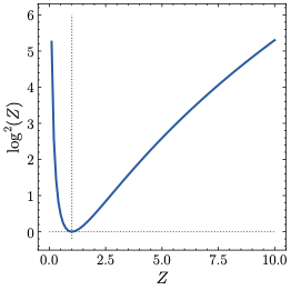
The z-loss term from Eq. ([eq:zloss]) is illustrated on the left hand side of Fig. 1. It incentivizes the model to create logits that fulfill $`Z \approx 1`$. To explore how this affects the logits themselves, we start by noting that there are two distinct mechanisms that can lead to a large z-loss $`\mathcal{L}_z`$, corresponding to $`Z \to 0`$ and $`Z \to \infty`$, respectively.
Lemma 1. *An infinite z-loss $`\mathcal{L}_z`$ corresponds to one of the following two (mutually exclusive) scenarios:
\begin{align}
&(i) \ &\exists~j \in [1, V]: l_j \to + \infty& \nonumber \\
&(ii) \ &\forall~j \in [1, V]: l_j \to - \infty& \nonumber
\end{align}
```*

</div>

<div class="proof">

*Proof.* *(i)* The statement is equivalent to $`Z \to \infty`$, from
which follows $`\mathcal{L}_z \to \infty`$. *(ii)* The statement is
equivalent to $`\forall~j \in [1, V]: \exp \left( l_j \right) \to 0`$,
which in turn is equivalent to $`Z \to \infty`$. From this follows
$`\mathcal{L}_z \to \infty`$. ◻

</div>

Both conditions in Lemma <a href="#lemma:1" data-reference-type="ref"
data-reference="lemma:1">1</a> have in common that the largest logit
diverges. They can be succinctly unified by the following statement.

<div id="theorem_zloss" class="proposition">

**Proposition 2**. *An infinite z-loss $`\mathcal{L}_z`$ corresponds to
``` math
\begin{align}
\max_j l_j \to \pm \infty
\end{align}
```*

</div>

<div class="proof">

*Proof.* Follows directly from
Lemma <a href="#lemma:1" data-reference-type="ref"
data-reference="lemma:1">1</a>. ◻

</div>

Consequently, z-loss prevents any *single* logit from positively
diverging, and all logits from negatively diverging *collectively*.
Notably, it does *not* prevent any single logit from diverging
negatively.

## Output Embeddings and Logits

Following the discussion on z-loss, we examine the relationship between
the output embeddings $`e_i`$ and logits $`l_i`$. In particular, we
consider their means and ranges. This will serve as a basis for the
subsequent introduction of our output embedding centering methods.

The connection between the mean word embedding
``` math
\begin{align}
\mu&= \frac{1}{V} \sum_{i=1}^V e_i
\label{eq:mu}
\end{align}and the mean logit
\begin{align}
\overline{l}
&= \frac{1}{V} \sum_{i=1}^V l_i
\label{eq:meanlogit}
\end{align}is expressed by the following lemma.
Lemma 3. *The mean logit is proportional to the mean embedding:
\begin{align}
\overline{l}&= \mu\mathpalette\mathbin{\vcenter{\hbox{\scalebox{h}{$\m@th.5\bullet$}}}}
\label{eq:mean_logit_expression}
\end{align}
```*

</div>

<div class="proof">

*Proof.*
``` math
\begin{align}
\overline{l}
&\stackrel{(\ref{eq:lmhead_logits})}{=} \frac{1}{V} \sum_{i=1}^V \left( e_i \mathpalette\mathbin{\vcenter{\hbox{\scalebox{h}{$\m@th.5\bullet$}}}} \right)
= \left( \frac{1}{V} \sum_{i=1}^V e_i \right) \mathpalette\mathbin{\vcenter{\hbox{\scalebox{h}{$\m@th.5\bullet$}}}}
\stackrel{(\ref{eq:mu})}{=} \mu\mathpalette\mathbin{\vcenter{\hbox{\scalebox{h}{$\m@th.5\bullet$}}}} \nonumber
\end{align}Note that in the second step, the linearity of the dot product was used. ◻
The impact of the word embeddings on the range of the logits is summarized by the following lemma.
Lemma 4. *The logits $`l_j`$ are globally bounded by
\begin{align}
- \max_i \| e_i \| \cdot \| h \| \leq l_j \leq \max_i \| e_i \| \cdot \| h \|
\label{eq:bounds_logit_expression}
\end{align}
```*

</div>

<div class="proof">

*Proof.* Follows directly from
$`l_j \stackrel{(\ref{eq:lmhead_logits})}{=} e_i \mathpalette\mathbin{\vcenter{\hbox{\scalebox{h}{$\m@th.5\bullet$}}}} = \| e_i \| \| h \| \cos \alpha_i`$,
where $`\alpha_i`$ is the angle between $`e_i`$ and $`h`$. ◻

</div>

In summary, the mean output embedding directly impacts the mean logit,
and the norms of the output embeddings define the range of the logits.
Hence, controlling the output embeddings provides a means to control the
logits. This insight lays the foundation for *output embedding
centering* (OEC). The idea behind OEC is to ensure that the mean output
embedding $`\mu`$ (cf. Eq. (<a href="#eq:mu" data-reference-type="ref"
data-reference="eq:mu">[eq:mu]</a>)) is bound to the origin, suppressing
the common shift of the embeddings
(cf. Sec. <a href="#sec:introduction" data-reference-type="ref"
data-reference="sec:introduction">1</a>) and uncontrolled logit growth.
OEC comes in two variants, *$`\mu`$-centering* and *$`\mu`$-loss*, which
we will introduce next.

## $`\mu`$-centering

OEC can be implemented in a deterministic, hyperparameter-free manner by
subtracting the mean output embedding $`\mu`$ from each output embedding
$`e_i`$, creating new output embeddings $`e_i^\star`$ after each
optimization step:
``` math
\begin{align}
e_i^\star &= e_i - \mu
\label{eq:output_embedding_centering}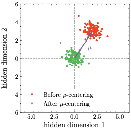
\end{align}This variant, called $`\mu`$-centering, is illustrated in the center panel of Fig. 1. It has some simple implications that can be summarized as follows:
Proposition 5. Let $`l`$ and $`\overline{l^\star}`$ denote the mean output logits before and after $`\mu`$-centering, respectively.
-
*The mean output logit after $`\mu`$-centering is zero:
MATH\begin{align} \overline{l^\star}= 0 \end{align} ```*Click to expand and view more -
*The output logits standard deviation is not affected by $`\mu`$-centering:
MATH\begin{align} \sigma_{l^\star}= \sigma_l \end{align} ```*Click to expand and view more -
The output probabilities and the loss are not affected by $`\mu`$-centering.
Proof. (i) Follows from Lemma 3 and Eq. ([eq:output_embedding_centering]). (ii) Follows from the shift-invariance of the standard deviation. (iii) Follows from the shift-invariance of the softmax. ◻
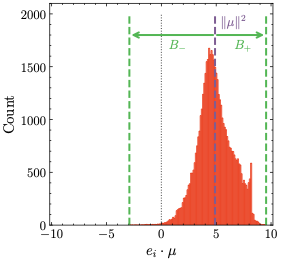
However, $`\mu`$-centering also has a less obvious, yet considerably more important, effect: it reduces the global logits bound subject of Lemma 4, thereby suppressing the unlimited growth of $`| l_i |`$ that can lead to divergences. Before we formalize this statement in Theorem 6, let us introduce some notation and build up an intuition for how this works in detail. We start by considering the dot products between each individual output embedding and the mean output embedding:
\begin{align}
e_i \mathpalette\mathbin{\vcenter{\hbox{\scalebox{\mu}{$\m@th.5\bullet$}}}}
\label{eq:output_embedding_dot_products}
\end{align}A histogram of these dot products is shown on the right hand side of Fig. 1.
 />
/>  />
/>  />
/>
As one can see, the typical distribution of the dot products approximates a skewed normal distribution centered around $`\| \mu\|^2`$. More importantly, it is bounded between $`\| \mu\|^2 - B_-`$ and $`\| \mu\|^2 + B_+`$ for some suitably chosen positive parameters $`B_-`$ and $`B_+`$. Under certain conditions (to be specified below), $`\mu`$-centering reduces the bounds for the dot products. This in turn leads to reduced bounds for the norm of the embeddings and the output logits. We will concretize and formalize this in the following theorem now.
Theorem 6. *Let $`B_-, B_+\in \mathbb{R}`$ be bounds such that
\begin{align}
\| \mu\|^2 - B_-\leq e_i \mathpalette\mathbin{\vcenter{\hbox{\scalebox{\mu}{$\m@th.5\bullet$}}}}\leq \| \mu\|^2 + B_+
\label{eq:bounds_before_oec}
\end{align}where $`\mu`$ represents the mean output embedding. Define the (non-negative) ratio
\begin{align}
B_{\rm ratio}&= \frac{\max(B_-, B_+)}{\max(B_-- \| \mu\|^2, B_++ \| \mu\|^2)}
\label{eq:Bratio_definition}
\end{align}and denote the mean output logits before and after $`\mu`$-centering by $`l`$ and $`\overline{l^\star}`$, respectively. Finally, $`e_i^\star`$ are the output embeddings after $`\mu`$-centering. Then
\begin{align}
B_{\rm ratio}\leq 1
\quad \Leftrightarrow \quad
\max \big| l_i^\star\big| \leq \max \big| l_i \big|
\label{eq:theorem_oec_condition}
\end{align}
```*

</div>

<div class="proof">

*Proof.* The bounds of
$`e_i^\star \mathpalette\mathbin{\vcenter{\hbox{\scalebox{\mu}{$\m@th.5\bullet$}}}}`$
after $`\mu`$-centering are
``` math
\begin{align}
- B_-&\leq e_i^\star \mathpalette\mathbin{\vcenter{\hbox{\scalebox{\mu}{$\m@th.5\bullet$}}}}\leq B_+
\label{eq:bounds_after_oec}
\end{align}From Eq. ([eq:bounds_before_oec]) and Eq. ([eq:bounds_after_oec]) we conclude that the respective bounds for the maximum of the absolute values of the dot products are
\begin{align}
\max_i \big| e_i \mathpalette\mathbin{\vcenter{\hbox{\scalebox{\mu}{$\m@th.5\bullet$}}}}\big| &= \max(B_-- \| \mu\|^2, B_++ \| \mu\|^2) \nonumber \\
\max_i \big| e_i^\star \mathpalette\mathbin{\vcenter{\hbox{\scalebox{\mu}{$\m@th.5\bullet$}}}}\big| &= \max(B_-, B_+)
\end{align}respectively. Hence, Eq. ([eq:Bratio_definition]) can be written as
\begin{align}
B_{\rm ratio}&= \frac{\max_i \big| e_i^\star \mathpalette\mathbin{\vcenter{\hbox{\scalebox{\mu}{$\m@th.5\bullet$}}}}\big|}{\max_i \big| e_i \mathpalette\mathbin{\vcenter{\hbox{\scalebox{\mu}{$\m@th.5\bullet$}}}}\big|}
\label{eq:Bratio_alternative}
\end{align}We will first prove the sufficiency ($`\Rightarrow`$) part of Eq. ([eq:theorem_oec_condition]). $`B_{\rm ratio}\leq 1`$ is equivalent to
\begin{align}
\max_i \big| e_i^\star \mathpalette\mathbin{\vcenter{\hbox{\scalebox{\mu}{$\m@th.5\bullet$}}}}\big| \leq \max_i \big| e_i \mathpalette\mathbin{\vcenter{\hbox{\scalebox{\mu}{$\m@th.5\bullet$}}}}\big|
\label{eq:theorem_oec_part1}
\end{align}which can also be written as
\begin{align}
\max_i \big| e_i^\star \mathpalette\mathbin{\vcenter{\hbox{\scalebox{\hat{\mu}}{$\m@th.5\bullet$}}}}\big| \leq \max_i \big| e_i \mathpalette\mathbin{\vcenter{\hbox{\scalebox{\hat{\mu}}{$\m@th.5\bullet$}}}}\big|
\label{eq:theorem_oec_part2}
\end{align}with the unit vector $`\hat{\mu}= \mu/ \| \mu\|`$. Let us now consider $`e_i^\star`$ and decompose it into the sum
\begin{align}
e_i^\star = e_i^{\star\parallel} + e_i^{\star\perp}
\end{align}of two vectors
\begin{align}
e_i^{\star\parallel} &= \left( e_i^\star \mathpalette\mathbin{\vcenter{\hbox{\scalebox{\hat{\mu}}{$\m@th.5\bullet$}}}}\right) \cdot \hat{\mu}
\label{eq:ei_decomposition_parallel} \\
e_i^{\star\perp} &= e_i^\star - \left( e_i^\star \mathpalette\mathbin{\vcenter{\hbox{\scalebox{\hat{\mu}}{$\m@th.5\bullet$}}}}\right) \cdot \hat{\mu}
\end{align}parallel and perpendicular to the mean embedding. This leads to
\begin{align}
\max_i \| e_i^\star \|^2
&= \max_i \| e_i^{\star\parallel} + e_i^{\star\perp} \|^2 \nonumber \\
&= \max_i \| e_i^{\star\parallel} \|^2 + \max_i  \| e_i^{\star\perp} \|^2
\label{eq:theorem_oec_decomposition}
\end{align}since $`e_i^{\star\parallel} \mathpalette\mathbin{\vcenter{\hbox{\scalebox{e}{$\m@th.5\bullet$}}}}_i^{\star\perp} = 0`$. The same decomposition can be conducted for $`e_i`$. However, the perpendicular component is not affected by $`\mu`$-centering, $`e_i^{\star\perp} = e_i^{\perp}`$, and neither is the second summand in Eq. ([eq:theorem_oec_decomposition]). Hence, we can write
\begin{align}
&\max_i \| e_i^\star \|^2 - \max_i \| e_i \|^2 \nonumber \\
&= \max_i \| e_i^{\star\parallel} \|^2 - \max_i \| e_i^\parallel \|^2 \nonumber \\
&= \max_i \big| e_i^\star \mathpalette\mathbin{\vcenter{\hbox{\scalebox{\hat{\mu}}{$\m@th.5\bullet$}}}}\big| - \max_i \big| e_i \mathpalette\mathbin{\vcenter{\hbox{\scalebox{\mu}{$\m@th.5\bullet$}}}}\big| \nonumber \\
&\leq 0
\end{align}where in the last two steps, Eq. ([eq:ei_decomposition_parallel]) and Eq. ([eq:theorem_oec_part1]) were used, respectively. Thus,
\begin{align}
\max_i \| e_i^\star \|^2
&\leq \max_i \| e_i \|^2
\end{align}The same holds for the (non-squared) norm of the mean embedding, which in turn leads to the right hand side of Eq. ([eq:theorem_oec_condition]) via Lemma 4:
\begin{align}
\max_i | l_i^\star | \leq \max_i | l_i |
\label{eq:Bratio_proof_rhs}
\end{align}The proof for the necessity ($`\Leftarrow`$) part of Eq. ([eq:theorem_oec_condition]) can be obtained by reversing the logic from Eq. ([eq:theorem_oec_part1]) to Eq. ([eq:Bratio_proof_rhs]). ◻
Importantly, the condition on $`B_{\rm ratio}`$ in Eq. ([eq:theorem_oec_condition]) is empirically fulfilled for all our experiments with the standard language modeling head, see App. 9.
$`\mu`$-loss
Instead of $`\mu`$-centering, we can also enforce OEC approximately by adding a regularization $`\mu`$-loss of the form
\begin{align}
\mathcal{L_\mu} &= \lambda \cdot \mu^\top \mu
\label{eq:mer}
\end{align}Here, $`\lambda \in \mathbb{R}^+`$ is a hyperparameter that is set to
\begin{align}
\lambda = 10^{-4}
\label{eq:lambda_default}
\end{align}by default, as in the case of z-loss (see Eq. ([eq:zloss])).
Proposition 7. *An infinite $`\mu`$-loss $`\mathcal{L}_\mu`$ corresponds to
\begin{align}
\max_j \big| l_j \big| \to \pm \infty
\label{theorem_muloss}
\end{align}
```*

</div>

<div class="proof">

*Proof.* Follows directly from
Eq. (<a href="#eq:mer" data-reference-type="ref"
data-reference="eq:mer">[eq:mer]</a>). ◻

</div>

Note the subtle difference compared to z-loss and
Proposition <a href="#theorem_zloss" data-reference-type="ref"
data-reference="theorem_zloss">2</a>: Absolute logits
$`\big| l_j \big|`$ appear in the limit instead of the logits $`l_j`$
themselves. Hence, $`\mu`$-loss suppresses the positive or negative
divergence of any single logit.
Tab. <a href="#tab:regularization_methods_effect" data-reference-type="ref"
data-reference="tab:regularization_methods_effect">1</a> summarizes the
methods discussed in this section, and the means by which they prevent
logit divergence.

<div id="tab:regularization_methods_effect">

<table>
<caption>Overview of methods and means by which logit divergences are
suppressed. Note that suppression of single divergences implies
suppression of collective divergences, but not vice versa.</caption>
<tbody>
<tr>
<td style="text-align: left;"></td>
<td style="text-align: center;"></td>
<td colspan="2" style="text-align: center;">suppressed divergence</td>
</tr>
<tr>
<td style="text-align: left;">name</td>
<td style="text-align: center;">type</td>
<td style="text-align: center;">positive</td>
<td style="text-align: center;">negative</td>
</tr>
<tr>
<td style="text-align: left;">z-loss</td>
<td style="text-align: center;">regularization</td>
<td style="text-align: center;">single</td>
<td style="text-align: center;">collective</td>
</tr>
<tr>
<td style="text-align: left;"><span
class="math inline"><em>μ</em></span>-loss</td>
<td style="text-align: center;">regularization</td>
<td style="text-align: center;">single</td>
<td style="text-align: center;">single</td>
</tr>
<tr>
<td style="text-align: left;"><span
class="math inline"><em>μ</em></span>-centering</td>
<td style="text-align: center;">centering</td>
<td style="text-align: center;">single</td>
<td style="text-align: center;">single</td>
</tr>
</tbody>
</table>

</div>

The theoretical advantages of $`\mu`$-loss and $`\mu`$-centering over
z-loss are the suppression of single negative logit divergences, their
simplicity, and the fact that they have a theoretical foundation that
addresses the root cause of the problem. Potential additional advantages
of $`\mu`$-centering over the regularization methods are that it is
hyperparameter-free and deterministic instead of stochastic. In
contrast, the regularization methods might offer more flexibility
compared to $`\mu`$-centering.

# Experiments

Our approach to studying training stability with regard to output logit
divergence primarily follows . In particular, we train dense decoder
models with a modern Transformer architecture on 13.1 billion tokens for
100000 steps, using 7 different learning rates:
``` math
\begin{align}
\eta \in \{ \text{3e-4, 1e-3, 3e-3, 1e-2, 3e-2, 1e-1, 3e-1} \}
\label{eq:eta}
\end{align}However, there are also a number of key differences. We use FineWeb and the GPT-2 tokenizer with a vocabulary size of $`V = 50304`$. Our 5 model sizes,
\begin{align}
N \in \{ 16{\rm M}, 29{\rm M}, 57{\rm M}, 109{\rm M}, 221{\rm M} \}
\label{eq:model_sizes}
\end{align}and the corresponding specifications (e.g. widths, number of layers and attention heads) are taken from . In addition, we use SwiGLU hidden activations and a non-truncated Xavier weight initialization . Further details on model architecture and hyperparameters are provided in App. 8. For each of the 7 x 5 = 35 combinations of learning rate and model size defined by Eq. ([eq:eta]) and Eq. ([eq:model_sizes]), we train four different models: A baseline model with the standard language modeling head (Sec. 1), and models using z-loss, $`\mu`$-loss as well as $`\mu`$-centering (Sec. 2). In order to compare the variants, we evaluate the dependency of the test loss on the learning rate and the dependency of learning rate sensitivity on the model size, with the latter defined as in :
\begin{align}
        {\rm LRS} &= \mathbb{E}_{\eta} \left[ \min (\mathcal{L}(\eta) , \mathcal{L}_0) - \min_\eta \mathcal{L} \right]
        \label{eq:lr_sensitivity}
\end{align}Here, $`\eta`$ are the learning rates from Eq. ([eq:eta]) and $`\mathcal{L}_0`$ denotes the loss at initialization time. Additionally, we investigate the dependency of a few other metrics on the learning rate for the purpose of analyzing the functionality of the different methods. Firstly, we consider the norm $`\| \mu\|`$ of the mean embedding (see Eq. ([eq:mu])). Secondly, we compute sample estimates for the mean logit $`\overline{l}`$ (see Eq. ([eq:meanlogit])), the logits standard deviation
\begin{align}
\sigma_l&= \frac{1}{V} \sum_{j=1}^V \left( l_j - \overline{l}\right)^2 \ ,
\end{align}as well as the maximum absolute logit
\begin{align}
\max_j |l_j| \ ,
\end{align}using $`5 \cdot 10^5`$ logit vectors created from the test data. Finally, the time $`t`$ to train a model on 4 A100 GPUs using data parallelism is compared.
Results
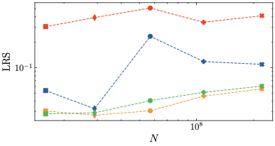
Training Stability
The main results of our experiments are shown in Tab. 4 and Fig 2.
| (i) Optimal Loss (↓) | |||||
|---|---|---|---|---|---|
| N | baseline | z-loss | μ-loss | μ-centering | |
| 16M | 3.84 | 3.84 | 3.84 | 3.84 | |
| 29M | 3.59 | 3.58 | 3.59 | 3.58 | |
| 57M | 3.37 | 3.37 | 3.37 | 3.37 | |
| 109M | 3.20 | 3.20 | 3.20 | 3.20 | |
| 221M | 3.05 | 3.05 | 3.05 | 3.05 | |
| (ii) Learning Rate Sensitivity (↓) | |||||
|---|---|---|---|---|---|
| N | baseline | z-loss | μ-loss | μ-centering | |
| 16M | 0.306 | 0.054 | 0.031 | 0.028 | |
| 29M | 0.391 | 0.033 | 0.027 | 0.029 | |
| 57M | 0.508 | 0.235 | 0.031 | 0.041 | |
| 109M | 0.344 | 0.118 | 0.046 | 0.051 | |
| 221M | 0.412 | 0.109 | 0.056 | 0.061 | |
| (iii) Additional Training Time (↓) | |||||
|---|---|---|---|---|---|
| N | baseline | z-loss | μ-loss | μ-centering | |
| 16M | 0.0% | 6.4% | 0.4% | 0.6% | |
| 29M | 0.0% | 4.3% | 0.7% | 0.5% | |
| 57M | 0.0% | 2.5% | 0.6% | 0.4% | |
| 109M | 0.0% | 1.5% | 0.4% | 0.4% | |
| 221M | 0.0% | 0.8% | 0.2% | 0.3% | |
 />
/>
 />
/>
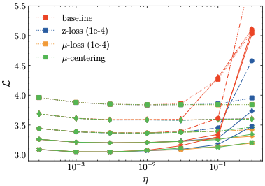
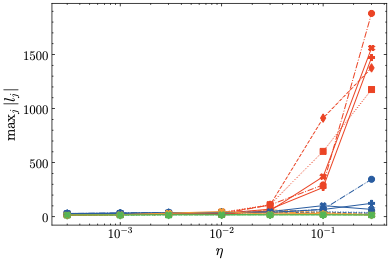
The top table (i) demonstrates that the optimal loss $`\min_\eta \mathcal{L}`$ for each model size is virtually the same for all methods. As expected, the top figure shows that the non-regularized baseline is the first to diverge with larger learning rates. Interestingly, z-loss leads to occasional divergences as well, given a large enough learning rate2. Meanwhile, none of the models using our methods diverge to any significant extent. This is also reflected in subtable (ii) of Tab. 4, which shows that $`\mu`$-loss and $`\mu`$-centering exhibit a lower learning rate sensitivity than z-loss, for all models sizes. In addition, subtable (iii) reveals that our methods are computationally cheap, such that the training time is minimally affected.
Analysis
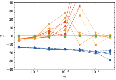
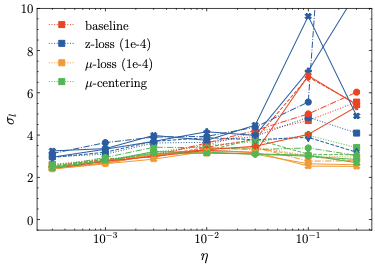
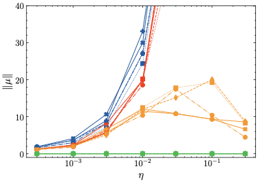
The additional metrics mentioned at the end of Sec. 3 are visualized in Fig. 3.
 />
/>  />
/>
 />
/>  />
/>
Firstly, regarding the logits mean (top left), we find that $`\mu`$-centering and $`\mu`$-loss center the logits at and around 0, respectively. Similarly, z-loss indirectly controls the logits mean, although at negative values. In contrast, the logits mean diverges at higher learning rates for the baseline, in accordance with the loss divergence observed in Fig. 2. Secondly, the standard deviation (top right) is the same for $`\mu`$-centering and the baseline barring slight statistical differences, at least for lower learning rates for which the baseline training converges. This is consistent with the theoretical prediction, see Proposition 5. In contrast, z-loss and $`\mu`$-loss—since they are regularization methods—change the logit standard deviation slightly. Thirdly, the mean embedding norm is shown on the bottom left. As expected, $`\mu`$-centering maintains a norm of zero while both baseline and z-loss grow at higher learning rates, indicating that z-loss fails to prevent anisotropic embeddings. Meanwhile, $`\mu`$-loss constrains the mean embedding norm to relatively small values. Finally, as predicted by Theorem 6, both $`\mu`$-centering and $`\mu`$-loss restrict the logit bound such that the maximum logit remains stable. Similarly, z-loss also implicitly restricts the maximum logit, albeit to a lesser degree than our methods, which explains the divergence observed for training using z-loss. In contrast, the maximum logit grows extremely large for the baseline models. In summary, these results are in accordance with the theoretical predictions from Sec. 2.
Hyperparameter Sensitivity
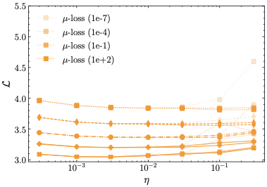
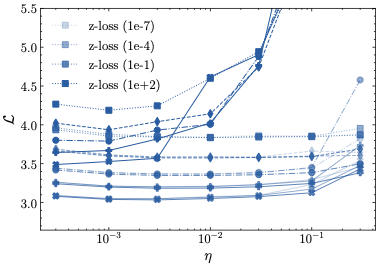
So far, the regularization hyperparameters have been set to their default value $`\lambda = 10^{-4}`$ for both regularization methods, z-loss (cf. Eq. ([eq:zloss])) and $`\mu`$-loss (cf. Eq. ([eq:lambda_default])). We now vary the regularization hyperparameter
\begin{align}
\lambda &\in \{ 10^{-7}, 10^{-4}, 10^{-1}, 10^{2} \}
\label{eq:lambda_ablations}
\end{align}for those methods, and determine the optimal loss and learning rate sensitivity as in Sec. 4 for each choice of $`\lambda`$. The results are presented in Tab. [tab:overview_comparison] and Fig. 8.
0.4 $`\mathbf{\mu}`$-loss
| (i) Optimal Loss (↓) | ||||
|---|---|---|---|---|
| N | 10−7 | 10−4 | 10−1 | 102 |
| 16M | 3.84 | 3.84 | 3.84 | 3.81 |
| 29M | 3.59 | 3.59 | 3.58 | 3.56 |
| 57M | 3.37 | 3.37 | 3.37 | 3.36 |
| 109M | 3.20 | 3.20 | 3.20 | 3.20 |
| 221M | 3.05 | 3.05 | 3.05 | 3.05 |
| (ii) Learning Rate Sensitivity (↓) | ||||
|---|---|---|---|---|
| N | 10−7 | 10−4 | 10−1 | 102 |
| 16M | 0.182 | 0.031 | 0.031 | 0.054 |
| 29M | 0.052 | 0.027 | 0.034 | 0.040 |
| 57M | 0.110 | 0.031 | 0.038 | 0.033 |
| 109M | 0.125 | 0.046 | 0.048 | 0.034 |
| 221M | 0.129 | 0.056 | 0.056 | 0.055 |
0.4 z-loss
| (i) Optimal Loss (↓) | ||||
|---|---|---|---|---|
| N | 10−7 | 10−4 | 10−1 | 102 |
| 16M | 3.84 | 3.84 | 3.83 | 4.19 |
| 29M | 3.59 | 3.58 | 3.57 | 3.94 |
| 57M | 3.37 | 3.37 | 3.35 | 3.79 |
| 109M | 3.20 | 3.20 | 3.18 | 3.64 |
| 221M | 3.05 | 3.05 | 3.03 | 3.49 |
| (ii) Learning Rate Sensitivity (↓) | ||||
|---|---|---|---|---|
| N | 10−7 | 10−4 | 10−1 | 102 |
| 16M | 0.037 | 0.054 | 0.032 | 1.156 |
| 29M | 0.044 | 0.033 | 0.043 | 1.780 |
| 57M | 0.107 | 0.235 | 0.047 | 1.392 |
| 109M | 0.076 | 0.118 | 0.059 | 2.150 |
| 221M | 0.131 | 0.109 | 0.101 | 2.166 |
μ-loss
 />
/>
z-loss
 />
/>
 />
/>
 />
/>
For $`\mu`$-loss, hyperparameter tuning is notably straightforward: the regularization coefficient only needs to be sufficiently large to enforce the centering effect. In fact, for larger values ($`\lambda \ge 10^{-4}`$), the training is stable and does not exhibit a strong dependency on the exact value of $`\lambda`$. Only when $`\lambda`$ is too small ($`\lambda = 10^{-7}`$), we observe that the loss diverges for large learning rates across all model sizes.
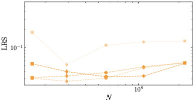
This behavior stands in contrast to z-loss, which requires more careful tuning. Severe divergences appear for $`\lambda=10^2`$, but also for lower values of $`\lambda`$ in conjunction with large learning rates. Our results indicate that the optimal value for z-loss is $`\lambda=10^{-1}`$, which is significantly larger than the previously assumed optimal value of $`10^{-4}`$. Importantly, however, even for the optimal $`\lambda`$, z-loss is outperformed by both $`\mu`$-loss and $`\mu`$-centering. This performance gap is evident in the learning rate sensitivity values for the largest model size $`N=221`$ in Tab. [tab:overview_comparison], as well as in the comparison of the rightmost points—corresponding to the largest model size—across the learning rate sensitivity plots in Fig. 8.
Conclusions
This paper establishes a link between the problems of anisotropic
embeddings and output logit divergence. We have identified the former as
the cause of the latter, and introduced $`\mu`$-centering and
$`\mu`$-loss as theoretically well-founded mitigation strategies. Our
experiments show that our methods outperform z-loss in terms of training
stability, learning rate sensitivity and hyperparameter sensitivity. The
code to reproduce our results is available at
github.com/flxst/output-embedding-centering
.
Limitations
We have only trained models up to a size of 221M parameters. In addition, our experiments use a fixed dataset, vocabulary size, token budget and set of hyperparameters. Hence, the same limitations as in apply. We have not investigated the dependency of the results on these factors, so we cannot make any reliable statements about their generalizability. Finally, while we have discussed the theoretical pros and cons of $`\mu`$-centering or $`\mu`$-loss in Sec. 2, we do not provide a clear recommendation on which method is to be preferred in practice.
Hyperparameters
All our experiments use the architecture and hyperparameters specified in Tab. 5.
| optimizer | AdamW |
| $`\beta_1`$ | 0.9 |
| $`\beta_2`$ | 0.95 |
| $`\epsilon`$ | 1e-8 |
| weight decay | 0.0 |
| gradient clipping | 1.0 |
| dropout | 0.0 |
| weight tying | false |
| qk-layernorm | yes |
| bias | no |
| learning rate schedule | cosine decay |
| learning rate minimum | 1e-5 |
| layer normalization | LayerNorm |
| precision | BF16 |
| positional embedding | RoPE |
| vocab size | 50304 (32101) |
| hidden activation | SwiGLU (GeLU) |
| sequence length | 2048 (512) |
| batch size (samples) | 64 (256) |
| batch size (tokens) | 131072 |
| training length | 100000 steps $`\approx`$ 13.1B tokens |
| warmup | 5000 steps $`\approx`$ 0.7B tokens |
| embedding initialization | Normal with standard deviation $`1/\sqrt{d}`$ |
| weight initialization | Xavier with average of fan_in and fan_out |
| (Xavier with fan_in, truncated) |
Architectural details and hyperparameters used in all our experiments. All settings match the ones from , with five exceptions. These are highlighted in bold, with the choice from being specified in parentheses.
Results for $`B_{\rm ratio}`$
As described in Sec. 3, we trained a total of 35 baseline models with a standard language modeling head (see Sec. 1), using 7 different learning rates (see Eq. ([eq:eta])) and 5 different model sizes (see Eq. ([eq:model_sizes])). Tab. 6 lists $`B_{\rm ratio}`$, as defined in Eq. ([eq:theorem_oec_condition]), individually for each of these models, while Fig. 9 shows a histogram of all its values.
| $`N`$ | 3e-4 | 1e-3 | 3e-3 | 1e-2 | 3e-2 | 1e-1 | 3e-1 |
|---|---|---|---|---|---|---|---|
| 4 | 0.97 | 0.82 | 0.75 | 0.62 | 0.66 | 0.26 | 0.65 |
| 6 | 0.98 | 0.82 | 0.92 | 0.73 | 0.49 | 0.30 | 0.44 |
| 8 | 0.96 | 0.81 | 0.79 | 0.67 | 0.60 | 0.66 | 0.57 |
| A | 0.97 | 0.74 | 0.67 | 0.74 | 0.72 | 0.61 | 0.70 |
| C | 0.95 | 0.74 | 0.84 | 0.91 | 0.68 | 0.70 | 0.70 |
$`B_{\rm ratio}`$ for all baseline models with a standard language modeling head. The numbers in the column header represent the learning rate $`\eta`$.
 />
/>
For each model, we find that the condition for Theorem 6 is fulfilled: $`B_{\rm ratio}\leq 1`$. Tab. 6 also shows that $`B_{\rm ratio}`$ tends to decrease with a larger learning rate. This indicates that the beneficial effect of $`\mu`$-centering (or $`\mu`$-loss) on the output logit bounds becomes larger, which is also in accordance with our results in Sec. 4.
📊 논문 시각자료 (Figures)
A Note of Gratitude
The copyright of this content belongs to the respective researchers. We deeply appreciate their hard work and contribution to the advancement of human civilization.Related Posts
Start searching
Enter keywords to search articles
No results found
Try using different keywords