Semantic change detection in remote sensing aims to identify land cover changes between bi-temporal image pairs. Progress in this area has been limited by the scarcity of annotated datasets, as pixel-level annotation is costly and time-consuming. To address this, recent methods leverage synthetic data or generate artificial change pairs, but out-of-domain generalization remains limited. In this work, we introduce a weak temporal supervision strategy that leverages additional temporal observations of existing single-temporal datasets, without requiring any new annotations. Specifically, we extend single-date remote sensing datasets with new observations acquired at different times and train a change detection model by assuming that real bi-temporal pairs mostly contain no change, while pairing images from different locations to generate change examples. To handle the inherent noise in these weak labels, we employ an object-aware change map generation and an iterative refinement process. We validate our approach on extended versions of the FLAIR and IAILD aerial datasets, achieving strong zero-shot and low-data regime performance across different benchmarks. Lastly, we showcase results over large areas in France, highlighting the scalability potential of our method.
💡 Summary & Analysis
1. **Key Contribution 1: Data Expansion**
This paper introduces a method to expand single-date annotated datasets like FLAIR and IAILD into bi-temporal pairs by adding new temporal acquisitions, significantly reducing the training cost for change detection models.
Key Contribution 2: Weakly Supervised Learning Framework
A weakly supervised learning framework is proposed that uses only single-date annotations to improve semantic change detection on bi-temporal image pairs without additional annotation costs.
Key Contribution 3: Strong Performance
Experiments across various datasets demonstrate significant improvements in the performance of change detection models, showcasing strong zero-shot and low-data regime results.
Detection and monitoring of changes in remote sensing data remain a
central topic within the Earth observation community over recent years .
A wide range of applications emerge from remote sensing change
detection, including natural disaster damage assessment , urban
development monitoring , or deforestation detection . In particular, the
task of bi-temporal change detection consists in finding the semantic
differences between a pair of co-registered satellite or aerial images
acquired at different dates, given a set of land cover classes of
interest.
State-of-the-art methods for this task use deep neural networks trained
on datasets of image pairs annotated with pixel-level change maps or
even semantic maps at both dates . Nevertheless, gathering such data is
both expensive and time consuming. As a result, change detection data is
often spatially or temporally clustered, and methods trained on them
hardly generalize to new, unseen locations. To address the scarcity of
labeled data, several works have attempted to train change detection
models in an unsupervised or weakly supervised fashion , learning from
much cheaper image-level annotations. However, these methods still lag
behind fully supervised approaches, particularly in the spatial accuracy
of predicted changes.
To benefit from quality semantic annotations at a larger scale, several
works attempt to leverage single-temporal annotated datasets in order to
train change detection model. This is the case of synthetic change
datasets generated from such existing data , but also of learning
frameworks considering non-overlapping images as training pairs ,
pairing images from different locations and thus generating fake change
pairs. However, such attempts do not take advantage of the growing
availability of remote sensing data. Satellite and aerial image
acquisition campaigns are indeed often programmed to occur regularly by
national GIS institutes or to last a long period of time by spatial
agencies .
In this paper, we propose to expand single-date semantic segmentation
datasets into bi-temporal collections, leveraging easily accessible
imagery. We introduce a new weakly supervised paradigm, where only
single-temporal semantic maps are available to train a change detection
network on bi-temporal pairs. Introducing this temporal variability
exposes the model to naturally occurring variations that do not
constitute semantically meaning changes, making it more robust. Because
this weak temporal supervision is by nature noisy, we propose three key
training ideas. First, we balance real bi-temporal pairs and fake
non-overlapping pairs during training. Secondly, inspired by , we
supervised fake pairs with an sIoU-based change map. Third, we
iteratively clean the extended dataset, filtering out real pairs
exhibiting land-cover changes, so that such pairs can be considered as
unchanged during training.
We validate our methodology by expanding two existing datasets, FLAIR
and IAILD . Through several experiments, we demonstrate that one can use
additional temporal acquisitions in addition to semantic segmentation
datasets to improve change detection with zero labeling cost. Our
contributions are summarized as follows:
We extend FLAIR and IAILD datasets from single-date to bi-temporal and
release them for anyone to use. We additionally curate and release a
test set for in-domain evaluation of building change detection methods
trained on our extension of FLAIR.
We develop an approach to leverage the additional, non-annotated
images for training a change detection network.
Through extensive experiments on several datasets, we show that our
method improves the performance of change detection models. Thus, we
demonstrate strong zero-shot performance, impressive low-data regime
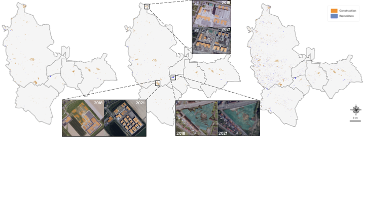
results, and compelling large-scale qualitative results, shown in
Fig. [fig:teaser].
Related Works
In this paper, we tackle the problem of detecting land cover changes in
bi-temporal remote sensing image pairs. We refer to this task as
semantic change detection (SCD).
Over the past few years, SCD in remote sensing images has gained
significant interest, leading to a large number of publications on the
topic and several field surveys . Most state-of-the-art methods rely on
deep learning in order to train 3-branch neural networks. First
introduced by Daudt et al. , such architectures output, for a given
bi-temporal image pair, a triplet consisting of two semantic maps and a
binary change map. Multiple variants improve different aspects of the
procedure, including the multitask objective , the fusion mechanisms ,
the consistency between the three outputs , the quality of the predicted
change boundaries , or the computational cost . All these methods
require pixel-level annotated image pairs in order to train a model in a
fully supervised manner. Because gathering such labeled data is costly
and time-consuming, we instead propose a weakly supervised framework
based on single-temporal annotations, leveraging new temporal images
without additional annotation cost.
Weakly supervised learning encompasses any training algorithm that
enables performing different or more complex tasks than typically
possible with the available data. However, in the context of SCD, it
specifically describes methods that infer pixel-level change predictions
from weak image-level labels . For instance, Andermatt et al. train a
SCD model with image-level labels such as “forests to agricultural
surfaces” for a given image pair. Between image- and pixel-level
supervision, other weak signals such as bounding boxes or coarse masks ,
noisy labels , and low-resolution annotations have been used to train
SCD networks. Toker et al. presented DynamicEarthNet , a dataset of
daily satellite image time series for which only the first image of each
month is annotated, with a focus on semi- rather than weak supervision.
Beyond this work, and to the best of our knowledge, weak settings in
which semantic information is completely missing for one image of the
pair are often overlooked in the literature, despite corresponding to
cases that commonly occur in practice due to the recurrent acquisition
of imagery by space and GIS agencies.
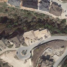
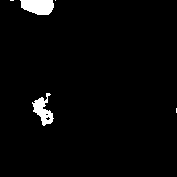
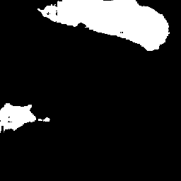
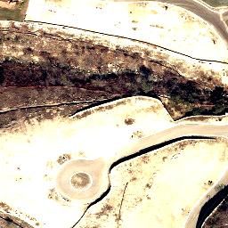
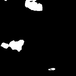
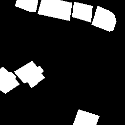
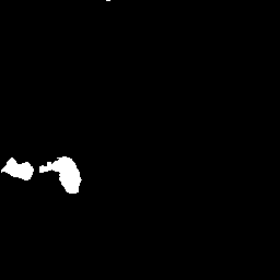
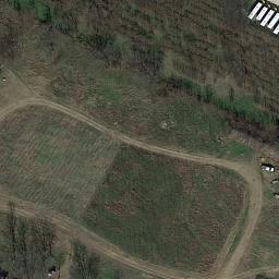
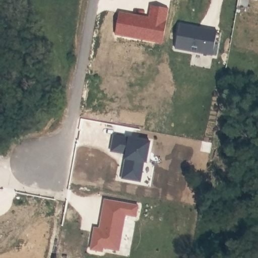
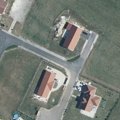
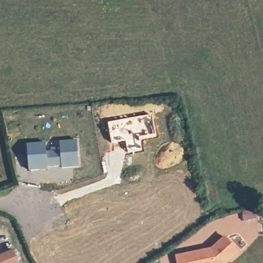
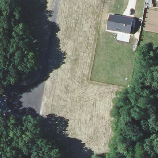
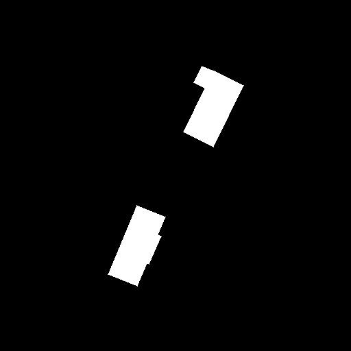
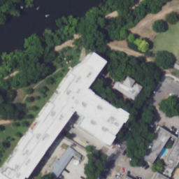
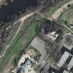
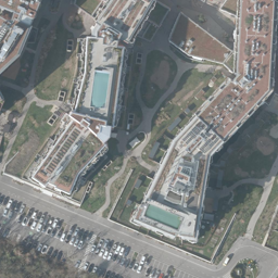
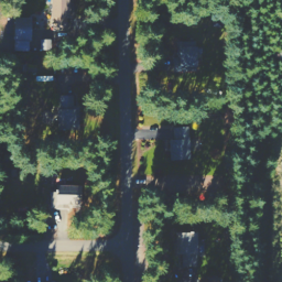
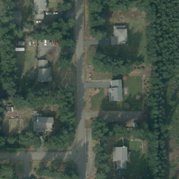
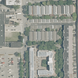
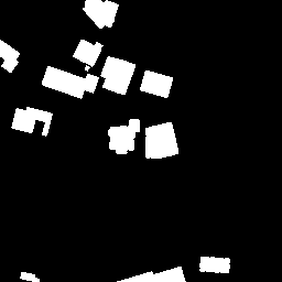
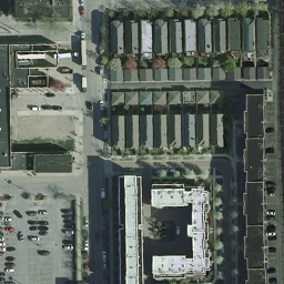
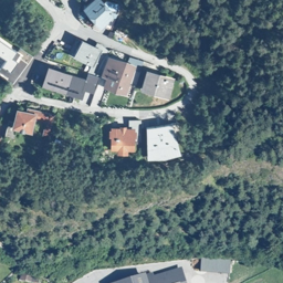
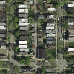
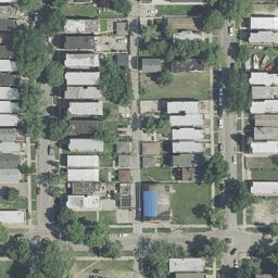
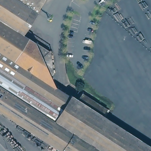
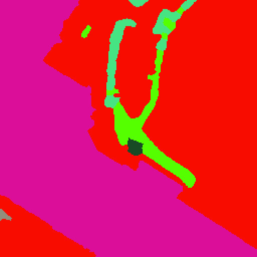
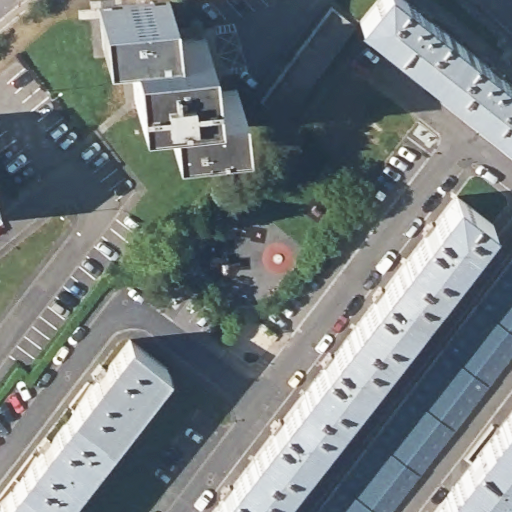
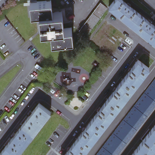
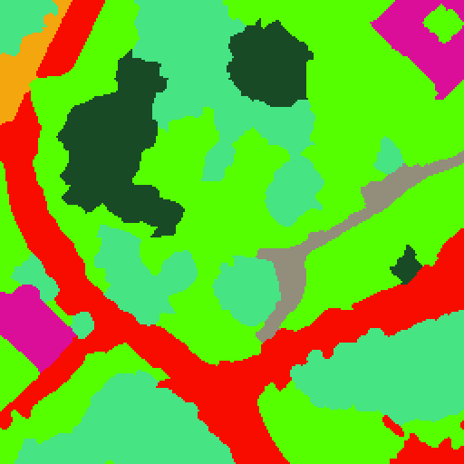
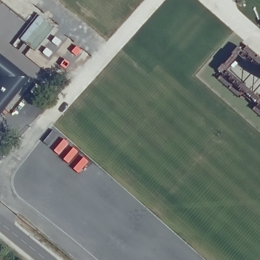
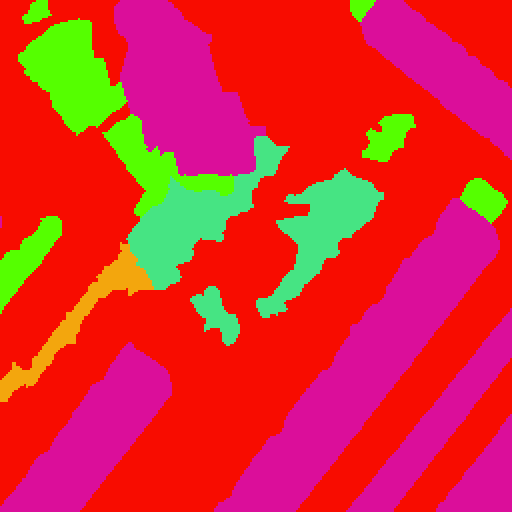
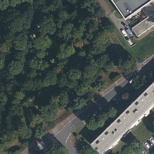
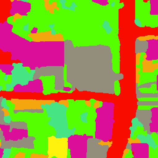
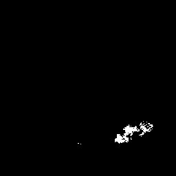
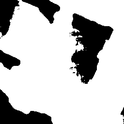
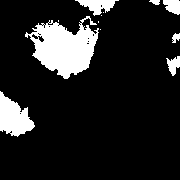
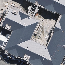
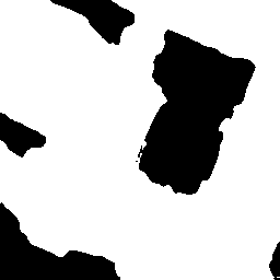
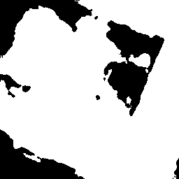
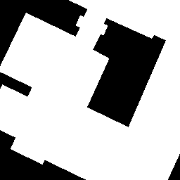
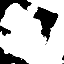
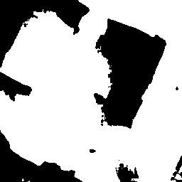
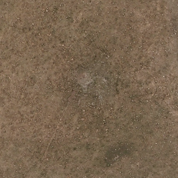
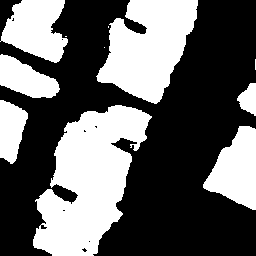
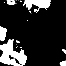
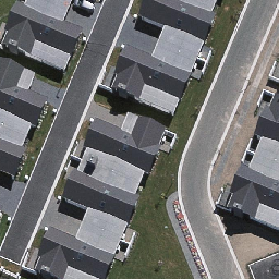
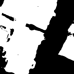
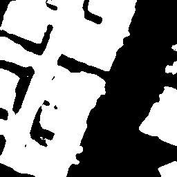
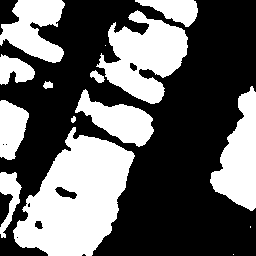
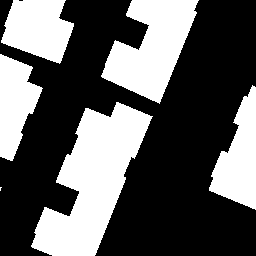
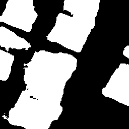
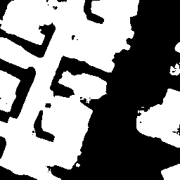
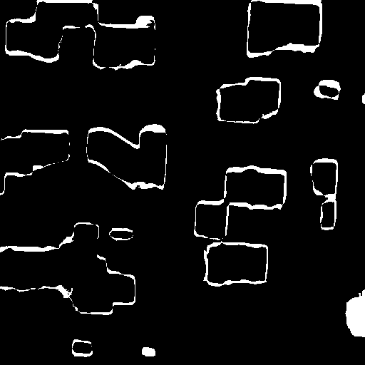
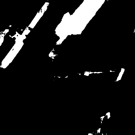
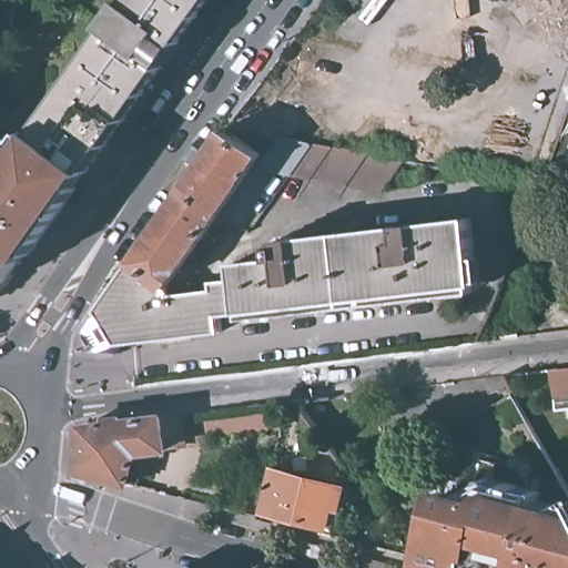
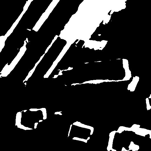
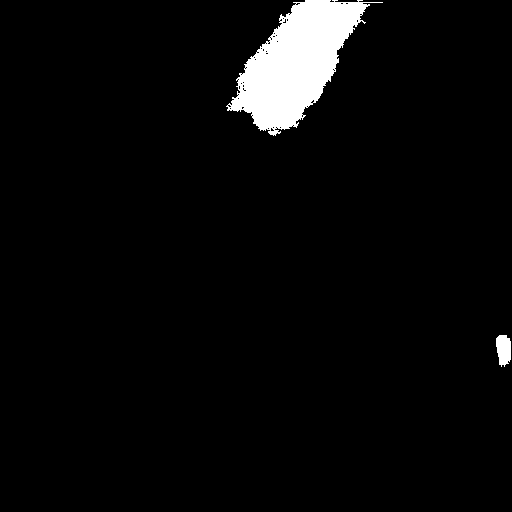
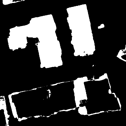
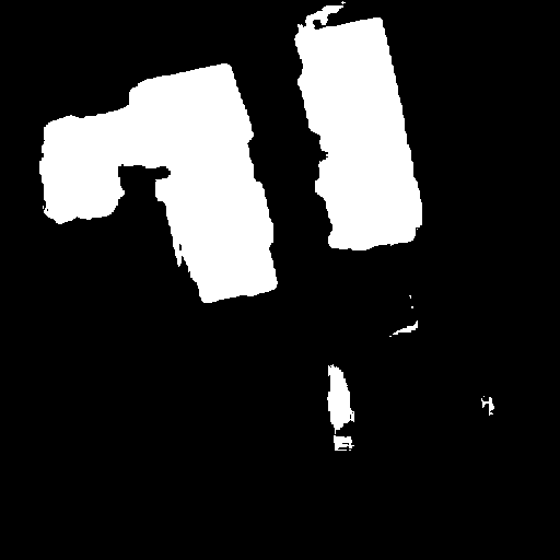
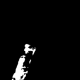
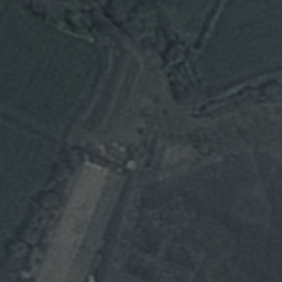
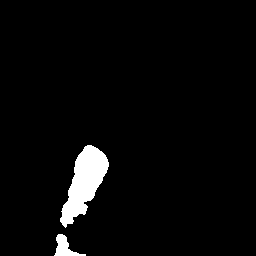
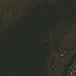
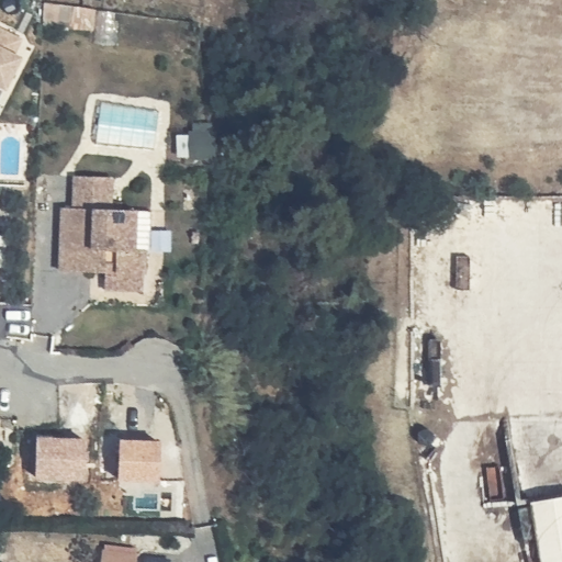
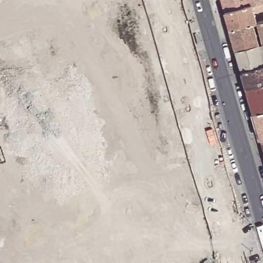
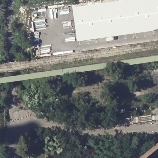
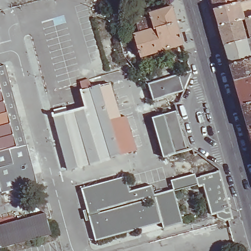
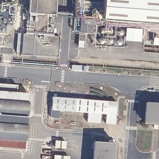
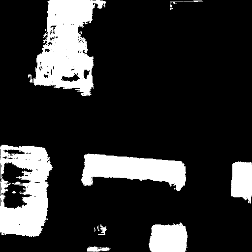
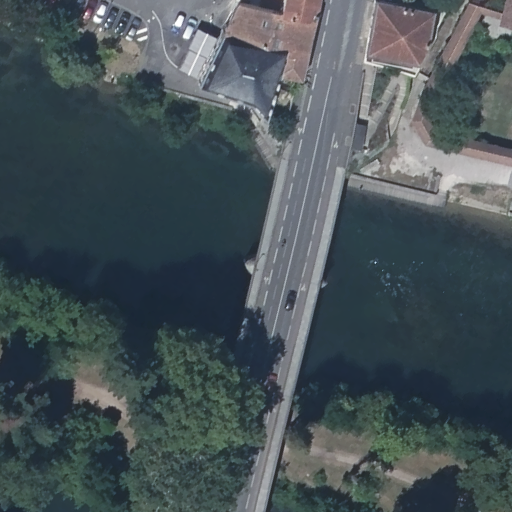
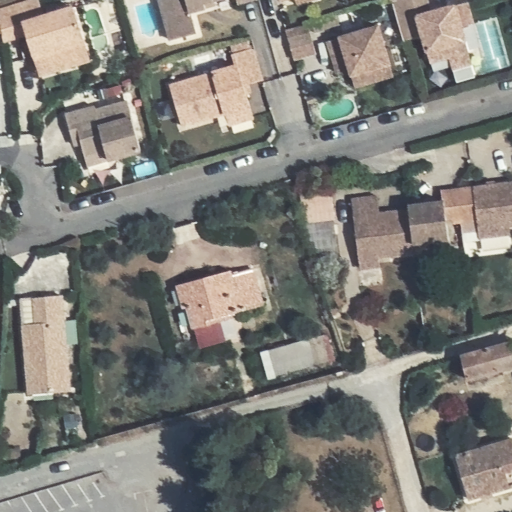
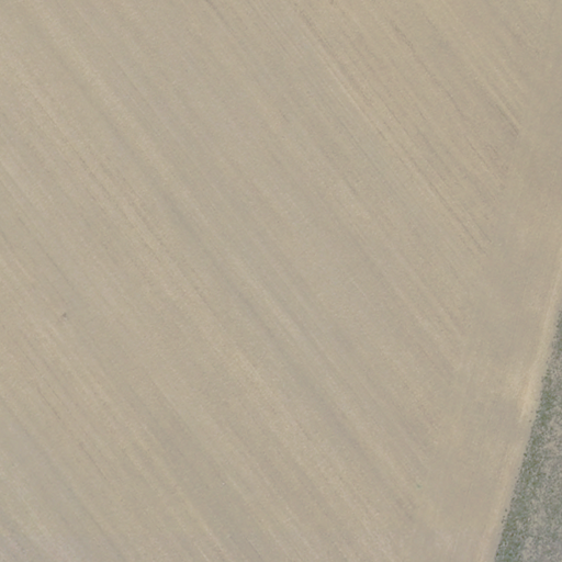
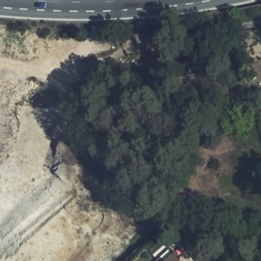
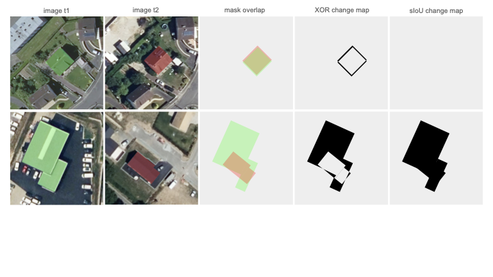
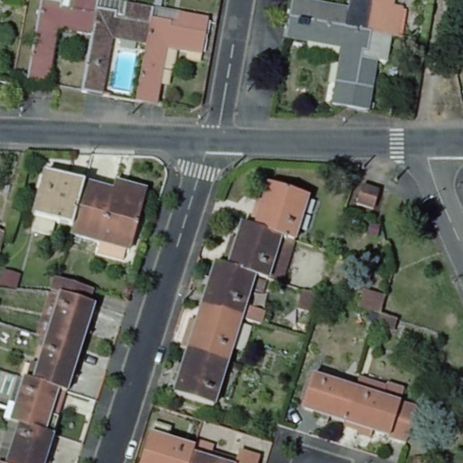
Visual examples. For each of the extended
datasets, we show example triplets (St, It, It′)
in this order from left to right, corresponding to the annotation mask,
the original image, and the added acquisition respectively. Pairs may
exhibit significant land cover changes (top row), or irrelevant changes
due to shadows or seasonal variations (middle and bottom
rows).
Due to the high cost of pixel-level change annotations, several works
have explored leveraging single-temporal semantic segmentation datasets
to enable change detection without requiring ground truth change labels.
A common approach is post-classification change detection, often
referred to as “the most obvious method of change detection” . It
compares the outputs of a single-temporal segmentation model on each
image of a bi-temporal pair. In this case, multi-temporal acquisitions
may serve as data augmentation at training time . However, this method
suffers from prediction error accumulation and lacks temporal modeling .
Other methods construct artificial change pairs by randomly pairing
images from different locations and computing change maps based on label
differences, STAR or . Another line of work consists in creating
synthetic SCD datasets based on a single-temporal land cover real-world
dataset, using techniques such as GANs , or diffusion . Building on the
observation that annotation is significantly more expensive than data
acquisition itself, we instead propose to extend existing
single-temporal datasets with new, aligned temporal acquisitions, using
their existing annotations as weak supervision for bi-temporal change
detection.
Methodology
We focus on learning to detect changes from a single-temporal satellite
or aerial image dataset annotated for the semantic segmentation task.
Based on the observation that accessing new acquisitions is less costly
than obtaining change labels, our pipeline starts by extending such
datasets temporally (Sec. 3.1). Then we leverage these new
bi-temporal pairs, along with the single-temporal annotations in order
to train a semantic change detection model
(Sec. 3.2). We detail our implementation in
Sec. 3.3.
Let $`\mathcal{D}`$ be a single-temporal dataset of $`N`$ aerial or
satellite annotated images $`I_{t_i}^i`$ in
$`\mathbb{R}^{C\times H\times W}`$ acquired at time $`t_i`$, for
$`i \in \{1, \ldots, N\}`$. $`C`$, $`H`$, and $`W`$ respectively refer
to the number of channels, height, and width of the images. Each
$`I_{t_i}^i`$ is annotated with a semantic mask $`S_{t_i}^i`$ in
$`\{1, ...,K\}^{H\times W}`$, with $`K`$ the number of semantic classes.
Now, let $`f_\theta`$ be a deep neural network with learnable parameters
$`\theta`$, returning, for a given input pair $`(I_{t}, I_{t'})`$ of
bi-temporal images, a change map of pixels whose semantic class changes
between the acquisition timestamps $`t`$ and $`t'`$. Our goal is to
train such a model $`f_\theta`$, using the dataset $`\mathcal{D}`$
extended with new, easily-available, non-annotated temporal acquisitions
$`I_{t'_i}`$.
Data
To verify our methodology, we apply it to two existing aerial datasets,
FLAIR and the Inria aerial image labeling dataset (IAILD) , spanning
areas in three countries (France, USA and Austria). Since we extend
these datasets so they contain bi-temporal pairs, we prepend their
name with “b-” to distinguish them from the original datasets.
FLAIR is based on aerial images from the French National Institute of
Geographical and Forest Information (IGN)’s BD ORTHO : a database of
aerial orthophotographies covering the French territory at 0.2 meters
per pixel (m/px). All $`512\times512`$ FLAIR image patches are annotated
with semantic maps that assign each pixel to one of 19 land cover
classes. BD ORTHO is renewed on average every three years, making it
possible to collect aerial images of the same locations at different
dates. We thus extract, for every FLAIR image, an additional observation
from the BD ORTHO database at around three years before or after the
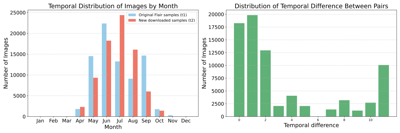
original FLAIR acquisition. b-FLAIR is challenging for weakly supervised
change detection with single-date annotations for two reasons. First,
FLAIR areas were selected for land cover diversity with no particular
temporal consideration, probably resulting in a low proportion of pairs
with relevant semantic change. Second, approximately 30% of pairs have
acquisition dates differing by two or more months, introducing seasonal
variations that, combined with varying acquisition times within the day,
may introduce significant radiometric and shadow changes.
IAILD covers urban areas in the USA and Austria. We only extended
IAILD’s training set, as its test set is not publicly available. It
consists of 180 patches of size $`5000\times5000`$ at a resolution of
0.3 m/px, annotated with binary building footprint masks. For each
location, we gathered a patch from the most recent available orthoimage
acquisition campaign released by the corresponding agency (USGS for the
USA, and the respective GIS agencies for Austrian provinces). The added
images have acquisition dates spanning 2022 to 2024, while IAILD’s
original images were acquired before 2017. Because the new acquisitions
have spatial resolutions varying from 0.15 to 0.6 m/px, we standardized
b-IAILD to 0.6 m/px. Due to IAILD’s urban focus, we expect b-IAILD to
contain more examples of changes related to artificialization and
building construction or demolition.
To verify our methodology beyond very high resolution aerial imagery, we
also created a satellite variant of b-FLAIR. For each bi-temporal pair,
we downloaded the corresponding SPOT-6/7 images from IGN’s ORTHO-SAT
database for the same acquisition year and location. The images have a
spatial resolution of 1.5 m/px, which we resampled to 1.6 m/px to obtain
$`64\times64`$ patches. The corresponding single-date semantic maps were
also resampled to the same resolution via nearest neighbor
interpolation. We refer to this satellite dataset as b-FLAIR-spot.
b-FLAIR, b-IAILD and b-FLAIR-spot thus contain triplets ($`S_{t}`$,
$`I_{t}`$, $`I_{t'}`$). We show example of such triplets in
Fig. 1. Further details on these
datasets, and additional example images can be found in the
Supplementary Material.
We evaluate competing methods on 5 datasets. For the in-domain
evaluation of methods trained on b-FLAIR and b-FLAIR-spot, we release
b-FLAIR-test and b-FLAIR-test-spot, two evaluation sets of 1730 image
pairs annotated with a binary building change mask. The images are in
the same format as FLAIR images and were acquired, processed, and
formatted following the procedure described in . The images were
extracted from 9 different French administrative departments and do not
intersect the FLAIR dataset, which allows for a sound evaluation of
methods trained on FLAIR or on our bi-temporal extensions of FLAIR. The
pairs were annotated by photointerpretation experts and verified by a
non-expert assessor. The pairs either show new building constructions,
or no building change at all ($`\thicksim`$30% of the pairs),
and no pair exhibits building destruction. For the out-of-domain
evaluation of all methods, we selected LEVIR-CD , WHU-CD , and
S2Looking , three datasets commonly used in building change detection
benchmarks. Hyperparameter studies are performed using a subset of
b-FLAIR for training, and b-FLAIR-test for evaluation. More details on
the evaluation can be found in the Supplementary Material.
Training with single date labels
Given a set of triplets
$`(S_{t_i}^i, I_{t_i}^i, I_{t_i'}^i)_{i=1,...,N}`$, our goal is to train
a bi-temporal change detection neural network $`f_\theta`$. Our
methodology can be applied to any model predicting, for an input image
pair ($`I_{t}`$, $`I_{t'}`$), a triplet ($`\hat{S}_{t}`$,
$`\hat{S}_{t'}`$, $`\hat{M}`$) respectively consisting of a semantic
mask for each frame and a binary change mask. A widely accepted
architecture for semantic change detection indeed consists of a
triple-branch network with two semantic segmentation branches and a
binary change branch. We now detail the three main components of our
training strategy: balanced batch sampling, change map generation, and
iterative refinement.
Our extended datasets typically contain a small fraction of pairs
exhibiting actual change events. Zheng et al. compensate the lack of
annotated change datasets in the literature by artificially pairing
images from different locations, using as change labels a difference of
their respective semantic masks. Building on this idea, we choose to mix
in a single batch such fake pairs with real bi-temporal pairs. We
thus introduce a parameter $`p_{\text{real}}`$ in $`[0,1]`$,
corresponding to the proportion of real pairs in each batch.
Specifically, for a batch of size $`B`$ of pairs
($`I_{t_i}^i, I_{t_i'}^i)_{i=1,...,B}`$ sampled from $`\mathcal{D}`$,
the method splits it into $`N_{\text{real}}`$ bi-temporal examples and
$`N_{\text{fake}}`$ unaligned examples, following:
MATH
\begin{equation}
N_{\text{real}} = \lfloor B \times p_{\text{real}} \rfloor~, \quad N_{\text{fake}} = B - N_{\text{real}}~.
\end{equation}
Click to expand and view more
We apply a random permutation to the $`N_{\text{fake}}`$ samples, such
that the image $`I_{t_i}^i`$ is paired with $`I_{t_j'}^j`$ with
$`j \neq i`$.
The models trained with our method usually supervise their predicted
maps ($`\hat{S}_t`$, $`\hat{S}_{t'}`$, $`\hat{M}`$) with ground-truth
maps ($`S_t`$, $`S_{t'}`$, $`M`$). In our weakly supervised setting, we
only have access to $`S_t`$. We create missing semantic and change maps
distinguishing two cases, depending on if the pair is real or fake. For
real pairs, we make the rough assumption that there is no semantically
relevant change between the two acquisitions, and define:
MATH
\begin{equation}
S_{t'} = S_t~, \quad M = 0~.
\end{equation}
Click to expand and view more
For fake pairs ($`I_{t_i}^i`$, $`I_{t_j'}^j`$), we use the semantic mask
of $`I_{t_j}^j`$ as proxy of the unavailable mask $`I_{t_j'}^j`$, again
assuming no change between the two acquisitions. In order to generate a
change mask $`M`$ from this pair of non-spatially aligned maps
$`S_{t_i}`$ and $`S_{t_j}`$, Zheng et al. apply an XOR operation,
which only consider the semantic temporal differences at the pixel
level. Instead, we choose to use an object-aware metric that considers
changes at the object level. To this end, we generate a change mask by
thresholding the sIoU between connected components of $`S_{t_i}`$ and
$`S_{t_j}`$. The sIoU is a well-adopted object-level variation of the
traditional intersection over union (IoU). Unlike the conventional IoU,
which penalizes fragmented ground truth regions by assigning each
prediction a moderate IoU score, the sIoU does not penalize predictions
for a segmentation if other predicted segmentations sufficiently cover
the remaining ground truth. This enables a robust evaluation of changes
at the object level, especially when accounting for shadow occlusions,
deformations, or label inconsistencies. Let $`\mathcal{C}_{t_i}`$ and
$`\mathcal{C}_{t_j}`$ denote the sets of connected components in
$`S_{t_i}`$ and $`S_{t_j}`$ respectively, where each component
corresponds to a semantic class. We compute the sIoU between each
component $`c^k`$ in $`\mathcal{C}_{t_i}`$, characterized by its
semantic category $`k`$, with respect to $`\mathcal{C}_{t_j}`$ as
The notation $`\left|\cdot\right|`$ denotes the size of a set in terms
of number of pixels. The term $`\mathcal{A}(c^k)`$ excludes from the
denominator any pixels belonging to other $`\mathcal{C}_{t_i}`$
components that overlap with $`c^k`$ and share the same semantic class
$`k`$, preventing interference from nearby objects. During training, we
apply this object-level comparison to each fake pair in the batch. For
each pair of semantic maps $`(S_{t_i}, S_{t_j})`$, we compute the sIoU
for all components in both directions: $`\mathcal{C}_{t_i}`$ with
respect to $`\mathcal{C}_{t_j}`$, and vice versa. A pixel location
($`x,y`$) of the binary change mask $`M`$ is labeled as a change if it
belongs to any connected component in either $`\mathcal{C}_{t_i}`$ or
$`\mathcal{C}_{t_j}`$ for which the sIoU is below a predefined threshold
$`\tau`$:
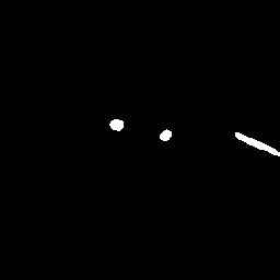
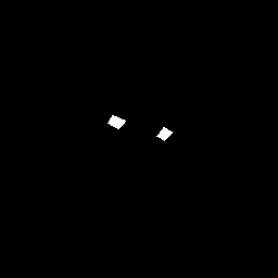
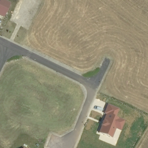
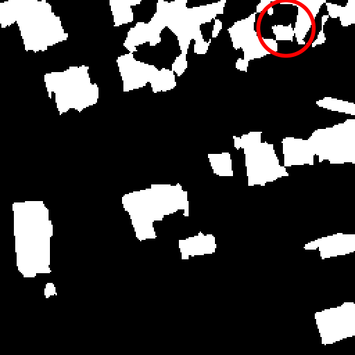
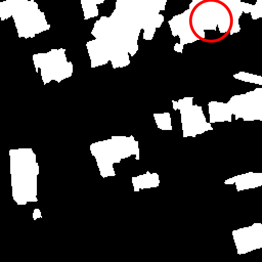
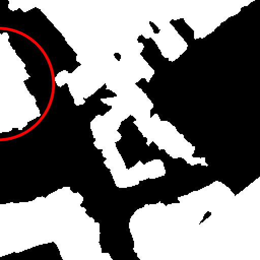
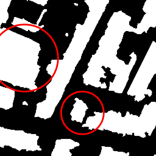
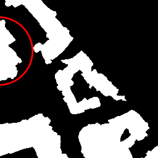
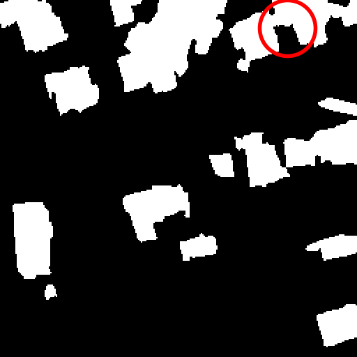
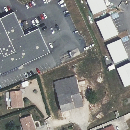
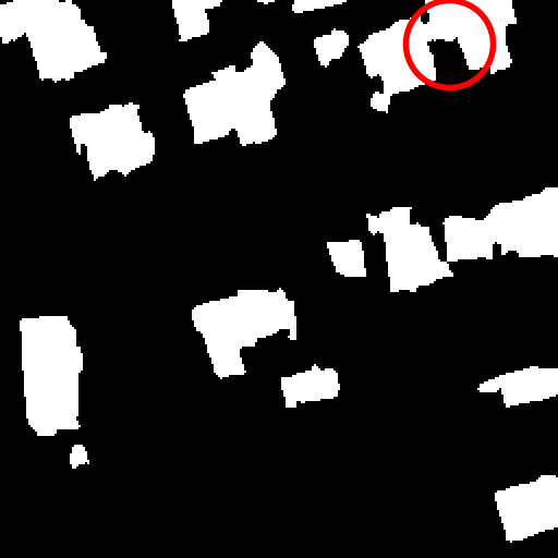
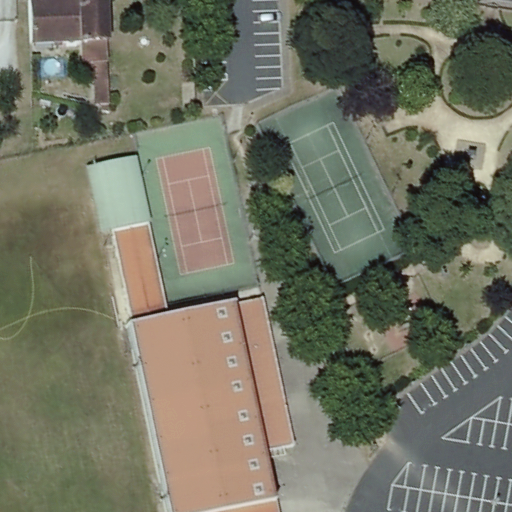
Fig. 2 provides a visual explanation of
the motivations and effects of the object-level change map generation
based on the sIoU. In particular, our method is consistent with labeling
co-registered real pairs with zero change maps, whereas XOR change maps
are sensitive to viewpoint changes.
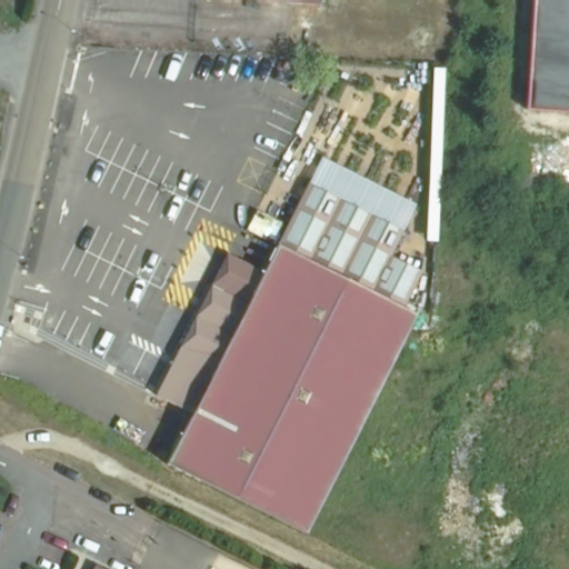
XOR vs. sIoU for change map generation from
image pairs, for the building change detection binary task. Top: a real
pair with slight viewpoint variation—XOR falsely detects changes, while
sIoU correctly shows none. Bottom: a fake pair with different
buildings—XOR misses overlapping changes, sIoU correctly marks both.
Only one building per image is labeled for clarity.
The rough assumption that real bi-temporal pairs can be labeled with a
zero change mask introduces noise in the supervision signal. Indeed,
genuine semantic changes may have occurred during the several years
separating the original and new acquisitions added in our extended
datasets. This leads to mislabeled training samples where changes are
incorrectly treated as unchanged, which can degrade model performance.
To mitigate this, we adopt an iterative refinement strategy. First, we
train a model on the entire dataset. We then use its predictions to
identify and filter out image pairs likely to contain changes. In
practice, we remove all image pairs for which the model predicts more
than 2% of changed pixels. In the next iteration, we train a model from
scratch using this cleaned dataset, therefore improving training
stability and overall prediction quality. We repeat this for
$`N_\text{iter}`$ iterations, where $`N_\text{iter}`$ is a
hyperparameter of the method. Ignoring a subset of the dataset by
removing noisy or incorrect samples, also known as data cleaning, has
been proven successful in other works .
Implementation
Recent analyses show that simple baselines like UNet remain highly
competitive for change detection despite the proliferation of complex
task-specific architectures . As architectural design is beyond the
scope of this paper, we adopt a 3-branch Dual UNet, following Benidir
et al . Note that the proposed methodology is architecture agnostic
and as such can also be applied to any 3-branch models.
We train our models in a multi-task setting, supervising the semantic
segmentation at both dates as well as the binary change detection with
corresponding focal losses. All models are trained using the AdamW
optimizer with a 1e-2 weight decay over 100 epochs and a learning rate
of 1e-4. We keep the model with the best validation IoU on the
segmentation task over the original sample $`t`$. We only use the RGB
bands of the images in the datasets, and focus on building change
detection when not explicitly stated otherwise. For example, with
FLAIR-based datasets, we ignore infrared and elevation bands, merging
all non-building classes into a “background” class. Our hyperparameters
are set to $`p_\text{real} = 0.25`$, $`\tau = 0.25`$, and
$`N_\text{iter} = 3`$.
Experiments
We compare our methodology with four frameworks that use single-temporal
semantic segmentation annotations for change detection. These include
post-classification with and without multi-temporal data augmentation,
synthetic dataset learning, and STAR , which generates fake change
pairs by pairing images from different locations in single-temporal
datasets. For post-classification, we train a UNet on the semantic
segmentation task and detect building changes by comparing bi-temporal
predictions. Bi-temporal data augmentation is achieved by using our
extended data during training. Lastly, we consider two Dual UNet
frameworks trained on synthetic datasets: SyntheWorld and FSC-180k .
We adopt F1-score (F1) and intersection over union (IoU) as evaluation
metrics for building change detection. These scores are reported as
percentages. We also report the false positive rates (FPR), and the
number and size of connected components to evaluate false alarms.
Image It
Image It′
Ground truth
Post-classif.
Post-classif.
FSC-180k
STAR
Ours
+ temp. aug.
pretraining
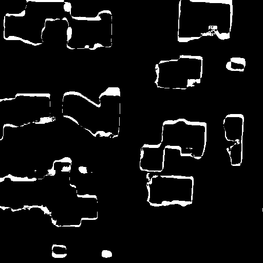
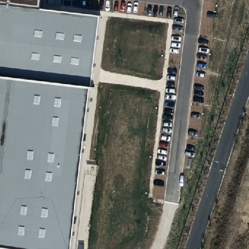
Qualitative results on b-FLAIR-test. We
compare the building change maps predicted by baseline methods and ours.
Tab. [tab:comparison_results]
reports in-domain performance on the b-FLAIR-test and b-FLAIR-test-spot
datasets (described in
Sec. 3.1), with qualitative examples in
Fig. 3. Our method achieves the
second-best score on b-FLAIR-test, while performance slightly drops on
b-FLAIR-test-spot. We attribute this to two main factors. (1) Our weak
supervision relies on temporal augmentation, which can introduce minor
misalignments or imperfect change annotations. This produces slightly
dilated predictions, smoother boundaries and less defined corners,
affecting IoU and F1 scores. (2) The model assumes most regions remain
unchanged between acquisitions, biasing predictions toward the no-change
class. Given change detection datasets are dominated by the background
class, false negatives penalize IoU and F1 more than false positives.
Beyond quantitative results,
Fig. 3 confirms that our model
is notably more robust in no-change regions, producing fewer false
positives. We argue that this behavior is desirable: in large-scale
deployments, minimizing false alarms is often more critical than
achieving perfectly sharp change boundaries. Therefore, we complement
our evaluation with an analysis of the FPR and connected components.
Tab. [tab:fpr_and_connected_components]
reports FPR, number of change connected components per image pair, and
average component size for our predictions, ground truth, and those of
Benidir et al. . Component-level evaluation treats small isolated
pixels equally to large false detections. While such small artifacts can
be easily removed through simple post-processing, larger false
detections are more challenging to handle. Following prior work , we
report results both before and after applying a 5×5 median filter on the
change maps. Across both metrics, our model produces substantially fewer
false positives, consistent with the qualitative large-scale results in
Fig. [fig:teaser], where our predictions
closely align with ground truth while FSC-180k shows numerous false
alarms.
We further evaluate zero-shot building change detection performance on
LEVIR-CD, WHU-CD, and S2Looking, as reported in
Tab. [tab:comparison_results].
Comparisons are made across models trained on the same data sources
(FLAIR, SPOT, and IAILD), with the best results highlighted for each
setting. Our method achieves the best overall performance on WHU-CD and
S2Looking, and consistently outperforms direct competitors within each
training domain. The only exception is the b-FLAIR variant on S2Looking,
which ranks second by a marginal difference. On LEVIR-CD, the
b-FLAIR-spot model surpasses its counterparts, although the b-FLAIR and
b-IAILD variants report lower performances. We also point out that these
datasets are “very” out-of-domain for models trained using FLAIR-spot
because of the difference in resolution ($`\sim1.6`$m vs $`\sim20`$cm).
Low data regime results. IoU scores on
LEVIR-CD and S2Looking datasets when fine-tuning a Dual UNet on limited
target data (1%, 10% and 30%). Each result is averaged over 10 runs.
Bold values denote the best performance for each dataset. †Results from .
Pretraining
Proportion of target data
used
2-4 dataset
1%
10%
30%
LEVIR-CD
2-4 No pre-training †
0.36
0.69
0.75
SyntheWorld†
0.41 (+14%)
0.71 (+3%)
0.77 (+3%)
FSC-180k†
0.55 (+53%)
0.73 (+6%)
0.79 (+5%)
b-FLAIR
0.60 (+67%)
0.77 (+12%)
0.81 (+8%)
b-IAILD
0.67 (+86%)
0.79 (+14%)
0.82 (+9%)
S2Looking
2-4 No pre-training†
0.10
0.27
0.38
SyntheWorld†
0.08 (-20%)
0.34 (+26%)
0.41 (+8%)
FSC-180k†
0.15 (+50%)
0.36 (+33%)
0.43 (+13%)
b-FLAIR
0.24 (+140%)
0.31 (+15%)
0.41 (+8%)
b-IAILD
0.27 (+170%)
0.37 (+37%)
0.41 (+8%)
We finetune a Dual UNet, pretrained with our methodology, on small
subsets of 1%, 10%, and 30% of training data for LEVIR-CD and S2Looking.
This evaluates the quality of the learned representations when training
with very few samples, a common practical scenario. Following the
protocol of Benidir et al. , we randomly sample training sets from the
target dataset and average results over 10 runs.
Tab. 1 reports results for our
b-FLAIR and b-IAILD models, compared with FSC-180k and SyntheWorld
from . Our approach achieves substantial improvements over the state of
the art when only minimal annotations are available (e.g., 1%), while
performance converges as more data is available.
Hyperparameters analysis
For the hyperparameters $`\tau`$ and $`p_\text{real}`$, we report the
scores of models trained on a subset of b-FLAIR.
0.35
0.65
XOR
sIoU
$`\tau`$
F1
IoU
—
76.0
61.3
0.75
74.8
59.7
0.50
73.1
57.8
0.25
77.0
62.6
Impact of $`p_\text{real}`$ and $`\tau`$. Left: Comparison of
different values for the proportion $`p_\text{real}`$ of real
bi-temporal pairs in training batches. Right: Comparison between XOR
change maps and our sIoU-based change maps computed with different
threshold $`\tau`$. Scores reported on b-FLAIR-test.
Tab. 2 shows adding
real pairs in a batch improves performance, with $`p_\text{real}=0`$
yielding the lowest scores. Performance peaks at $`p_\text{real}=0.25`$,
while higher values degrade it, likely because overrepresented real
pairs with no change bias the model toward predicting no change.
As shown in
Tab. 2, a threshold of
$`\tau=0.25`$ for sIoU-based change map generation outperforms the
logical XOR operation. On the contrary, higher thresholds
($`\tau \in \{0.5, 0.75\}`$) tend to classify components as changed
despite significant overlap between building footprints across the two
masks, resulting in noisy supervision. Note that $`\tau=1`$ reduces our
sIoU-based maps to the OR operation, which Zheng et al. demonstrated
to be inferior to XOR-based change maps for training change detection
models. Visualizations comparing these different change map generation
variants are provided in the Supplementary Material.
Performance across training iterations. F1
Score (%) and IoU (%) of a Dual UNet trained with our method over three
training iterations, and evaluated on the corresponding in-domain test
set. Best results per dataset are shown in bold.
b-FLAIR
b-FLAIR-spot
2-3(lr)4-5
F1
IoU
F1
IoU
Iteration 1
67.3
50.7
22.6
12.7
Iteration 2
78.1
64.1
21.7
12.2
Iteration 3
79.0
65.2
22.9
12.9
Our methodology relies on mixing bi-temporal image pairs with fake pairs
of unaligned images, while assuming by default that all real pairs
contain no change. This assumption is incorrect in practice in certain
cases, particularly since our extension of existing single-temporal
datasets is based on new acquisitions often captured several years
apart.
Tab. 3 therefore
demonstrates the benefit of iterative cleaning of the extended datasets,
through filtering of image pairs that would contain significant semantic
changes. For b-FLAIR, the second iteration increases F1 by over 10pt and
IoU by nearly 14pt on b-FLAIR-test, while gains at the third iteration
are smaller. We therefore set $`N_\text{iter} = 3`$ by default.
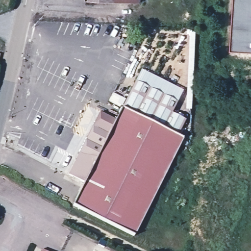
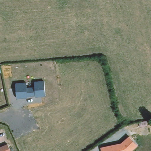
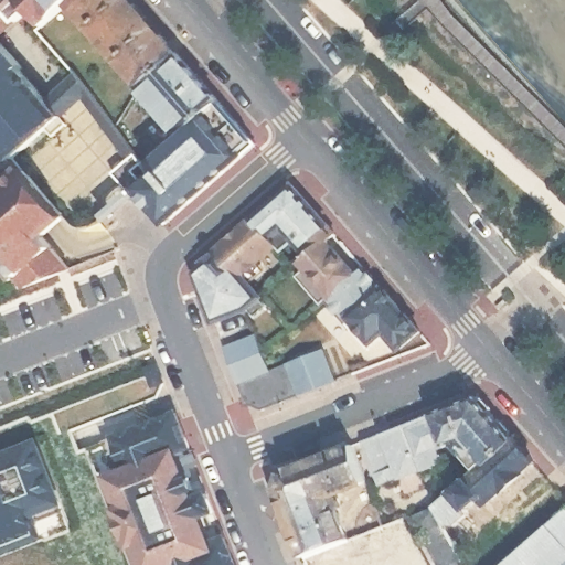
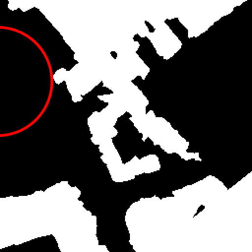
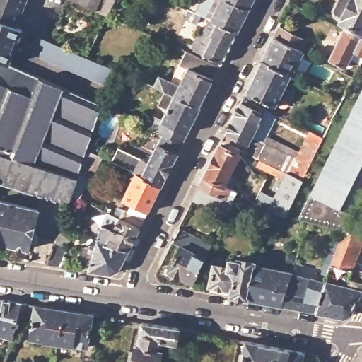
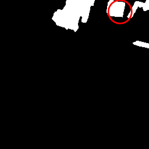
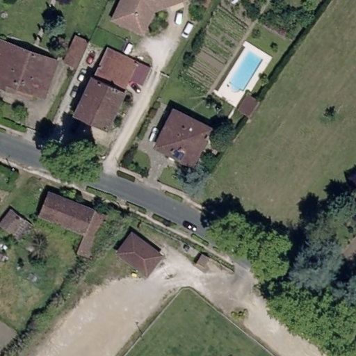
Fig. 4 illustrates filtered pairs,
including building changes and blurred sensitive areas. On b-FLAIR-spot,
successive iterations have little effect.
Samples removed during iterative
refinement. Triplets (It, It′,
M̂) removed during refinement
exhibit real building changes or blurred sensitive areas, where the
assumption M = 0 does not
hold. Such samples are correctly identified by the model and excluded
from the training set on subsequent iterations.
Conclusion
In this article, we introduced a novel approach for training remote
sensing change detection models by extending single-date datasets and
supervising changes through weak temporal supervision, without
additional annotations. We assume no change occurs between two
observations of the same location while providing change examples by
pairing images from different locations. Extensive experiments across
multiple datasets show that our methodology learns models with strong
out-of-distribution generalization, can be fine-tuned with minimal
annotations, and are robust to false positives in “in the wild”
scenarios. Qualitative results demonstrate strong alignment with ground
truth building construction and demolition maps, bridging the gap
between weak supervision and reliable large-scale change monitoring.
Overall, our framework offers a practical, annotation-efficient approach
to scalable change detection for both aerial and remote sensing
observations.
Acknowledgement
This work was funded by AID-DGA (l’Agence de l’Innovation de Défense à
la Direction Générale de l’Armement—Ministère des Armées), and was
performed using HPC resources from GENCI-IDRIS (grants
2023-AD011011801R3, 2023-AD011012453R2, 2023-AD011012458R2) and from the
“Mésocentre” computing center of CentraleSupélec and ENS Paris-Saclay
supported by CNRS and Région Île-de-France
(http://mesocentre.universite-paris-saclay.fr
).
Centre Borelli is also with Université Paris Cité, SSA and INSERM. This
work is additionally supported by RGC-GRF project 11309925, Mathematical
Formalization of GIS. We thank Etienne Bourgeat, Fabien Poilane and
Floryne Roche for their valuable assistance in data curation and
annotation.
We first provide additional details on the datasets used in this work
(Sec. 6). Then we detail our
implementation
(Sec. 7). Finally, we report
supplementary quantitative and qualitative results
(Sec. 8). Our code and
datasets will be released publicly for anyone to use.
Data
Fig. [fig:add_visual_examples]
shows further examples of triplets of bi-temporal images and their
corresponding single-temporal semantic masks, for our three extended
datasets, b-FLAIR, b-FLAIR-spot and b-IAILD. We describe them below, and
also give a brief description of the benchmark datasets we used
(LEVIR-CD, WHU-CD and S2Looking).
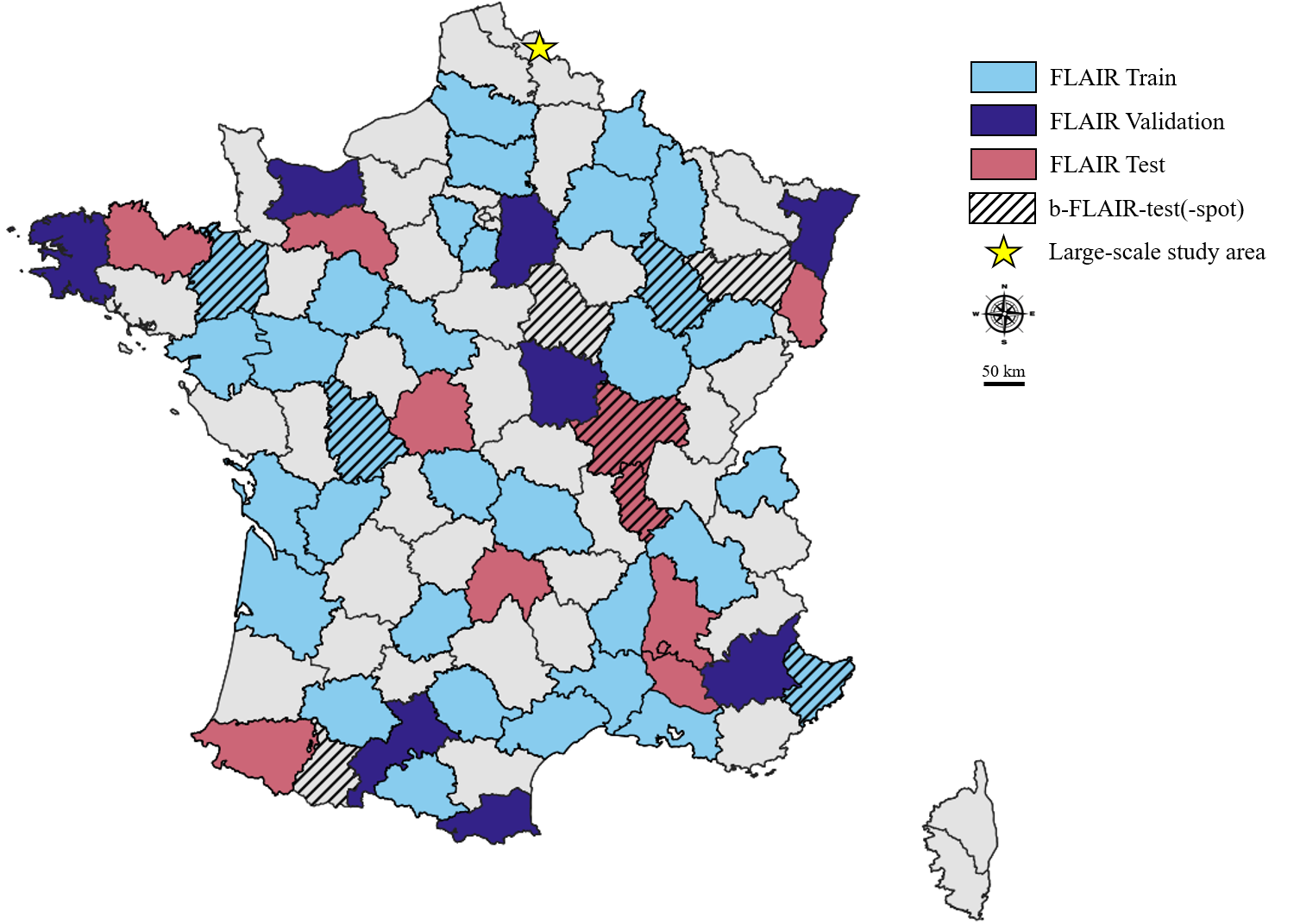
Spatial repartition of b-FLAIR-test(-spot) data
w.r.t. FLAIR, within Metropolitan France. Note that even if
pairs from b-FLAIR-test(-spot) are from departments already covered by
FLAIR, we made sure that there is no intersection between the two
datasets. We also indicate with a the location of the large-scale zone
used for Fig. 1 of the main paper.
b-FLAIR
The original FLAIR dataset is based on the French IGN’s BD ORTHO
product and its associated elevation data. For details on these data
products, their pre-processing and their formatting into the FLAIR
dataset, please refer to the FLAIR datapaper . The BD ORTHO product is
updated every three years on average at each location with new aerial
acquisitions. This allowed us to extend FLAIR dataset with a new
temporal acquisition for each of its 77,762 patches. For each patch, we
extracted a 5-band (RGB, infrared, elevation) patch from the closest
temporal acquisition of the BD ORTHO product and its associated
elevation data, following the same process as described in . We use the
same training splits as in the original paper (see
Fig. 5), except for the hyperparameter
studies for which a subset of the data is used (departments 13, 21, 44,
63, 80 for training, and 77 for validation). The average number of days
between two acquisitions is 1097 days ($`\thicksim`$3 years).
82.9% of our added images correspond to images acquired after the
corresponding original FLAIR patches, while the remaining were acquired
before. The average number of days between two acquisitions within the
same calendar year is 44 ($`\thicksim`$1.5 months), with 18% of
the pairs having more than a 3-month difference within the same calendar
year, indicating possible significant seasonal variations for a given
image pair. In addition, the differences in the time of the acquisitions
within the day—which is 153 min on average—and in the angle of
acquisition, introduce significant radiometric, geometric, and
shadow-related variations.
b-FLAIR-spot
For all patch location and acquisition date of b-FLAIR, we download a
corresponding SPOT-6/7 patch from the ORTHO-SAT database . These are RGB
images in 8 bits, at a spatial resolution of 1.5 m/px. We resized the
patches at the shape 64$`\times`$64, resulting in an effective
spatial resolution of 1.6 m/px. The ORTHO-SAT is an annual product, and
we align the acquisition year of the images of b-FLAIR-spot on the
corresponding images in b-FLAIR. This allows us to reuse FLAIR
annotations for b-FLAIR-spot, provided a nearest-neighbor resampling
from 512$`\times`$512 to 64$`\times`$64.
b-IAILD
The original IAILD public training set is composed of images from 5
cities from the USA (Austin, Chicago, Kitsap) and Austria (Tyrol,
Vienna). For each city, the dataset contains 36 tiles of size
5000$`\times`$5000 px at the spatial resolution of 30 cm/px. We
downloaded new acquisitions over the same locations from the USGS
website2 and the respective website of the Austrian provinces of
Tyrol3 and Vienna4. Years of acquisition of the new added
orthophotographies are the following : 2024 for Vienna, 2023 for
Chicago, Kitsap and Tyrol, and 2022 for Austin. Because the spatial
resolution varies across the areas of interest (15 cm/px for Vienna, 20
cm/px for Tyrol, and 60 cm/px for Austin, Chicago and Kitsap), we
resample all the downloaded tiles—as well as the original IAILD tiles—at
the common resolution of 60 cm/px. As in , we keep the first 5 tiles of
each zone for validation, and use the other 31 for training. The
resulting 2500$`\times`$2500 images are split in 100 patches of
size 256$`\times`$256, over a grid with an overlap of 6 pixels
between adjacent cells. This results in a dataset containing 15500
training pairs (3100 per area) and 2500 validation pairs (500 per area).
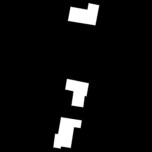
Examples triplets of our test sets for building
change detection. We show additional example triplets (It, It′,
M) in this order from top to
bottom, for b-FLAIR-test (a) and b-FLAIR-test-spot (b).
FSC-180k
STAR
Ours
Comparison with different architectures on
b-FLAIR-test. Like competing approaches, our methodology
can be applied to any 3-branch change detection
architecture.
FSC-180k
STAR
Ours
Comparison with different architectures on
WHU-CD. Like competing approaches, our methodology can
be applied to any 3-branch change detection architecture.
b-FLAIR-test & b-FLAIR-test-spot
b-FLAIR-test is composed of 1730 image pairs annotated with a binary
building change mask. The images are in the same 5-band
512$`\times`$512 format as FLAIR images and where acquired,
processed, and formatted following the procedure described in . The
images were extracted from 9 different French administrative departments
and do not intersect the FLAIR dataset, which allows for a sound
evaluation of methods trained on FLAIR or on our bi-temporal extension
of FLAIR (see Fig. 5). The pairs were annotated by
photointerpretation experts and verified by a non-expert assessor. The
pairs either show new building constructions, or no building change at
all ($`\thicksim`$30% of the pairs), but no pair exhibits
building destruction. b-FLAIR-test-spot is built from b-FLAIR-test
similarly as how we obtained b-FLAIR-spot based on b-FLAIR, i.e. by
downloading acquisition at the same date and location for each patch,
and downsampling the annotation masks. Example triplets for these two
datasets can be visualized in
Fig. 6.
LEVIR-CD, WHU-CD and S2Looking
is composed of 637 pairs of aerial images of size
1024$`\times`$1024 at the spatial resolution of 50 cm/px. We
keep the original data splits (445 images for training, 64 for
validation, and 128 for testing). LEVIR-CD’s images are from 20
different regions in the state of Texas, US, and were acquired between
2002 and 2018. The temporal gap for two acquisitions of the same
location in the dataset range from less than a year to 15 years.
is composed of 7620 pairs of aerial images of size
256$`\times`$256 at the spatial resolution of 7.5 cm/px. We keep
the original data splits (6096 images for training, 762 for validation,
and 762 for testing). WHU-CD’s images are of the area of Christchurch,
New Zealand, and were acquired in 2012 (pre-change) and 2016
(post-change).
is composed of 5000 pairs of satellite images of size
1024$`\times`$1024 at a spatial resolution between 50 cm/px and
80 cm/px. We keep the original data splits (3500 images for training,
500 for validation, and 1000 for testing). S2Looking’s images are from
15 areas of interest spread across Europe, Asia, Africa, and North and
South America. They were acquired between 2017 and 2020, with a temporal
gap ranging from 1 to 3 years between bi-temporal acquisitions.
Tab. [tab:datasets] summarizes the main
characteristics of these three datasets, as well as those of our two
datasets, b-FLAIR-test and b-FLAIR-test-spot.
Implementation details
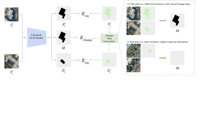
A general diagram of the proposed weak temporal supervision approach is
shown in Fig. 9. We trained the b-IAILD and
b-FLAIR-spot models on a single NVIDIA RTX 6000 GPU with batch sizes of
64 and 256, respectively. Training the b-IAILD model required
approximately 26 hours, while b-FLAIR-spot completed in about 5.5 hours.
The b-FLAIR dataset contains a significantly larger number of pixels
than the other datasets, resulting in substantially higher computational
complexity. Consequently, we trained the b-FLAIR models on a multi-GPU
setup with 32 NVIDIA V100 GPUs and a batch size of 32, where a complete
training took roughly 4 hours. For all models, we use image crops of
$`256 \times 256`$ pixels (except b-FLAIR-test, for which images are of
size $`64 \times 64`$) and normalize input images using the per-channel
mean and standard deviation computed over the entire training dataset,
following Benidir et al. . During inference and evaluation, target
images are normalized using the same statistics as the training set.
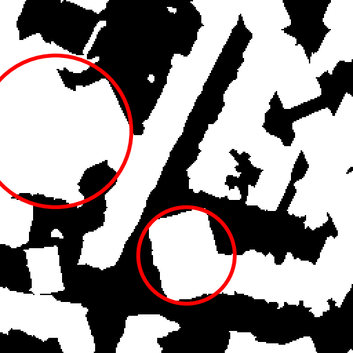
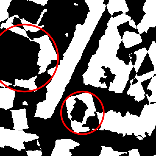
In Fig. 10, we show example of
change maps generated with our implemented sIoU-based methods. We
visually compare them to change maps computed with logical operations
(OR and XOR). While XOR-based masks leave residual change pixels around
almost-overlapping buildings, our masks ignore such pixels, though they
may correspond to an actual difference in land cover. We believe these
“cleaner”, object-based change masks constitute a better supervision in
order to train models that are less prone to false alarms.
/>
General diagram of the proposed
methodology. Our methodology can be applied to any 3-branch SCD
model, provided it can take two images at different dates as input and
produce a semantic segmentation mask for each date, and a change mask.
The semantic segmentation task is supervised through the single-temporal
available ground truth, implying a temporal augmentation on the
additional non-annotated image. The change detection task is supervised
via weak temporal augmentation, creating fake change examples
by pairing images of different locations, and no-change examples by
assuming no changes occurred between real pairs.Example of generated change maps for pairs
of images of b-FLAIR from different locations, with a focus on the
“building class”. We show maps resulting from logical operations (XOR or
OR) as well as sIoU-based maps computed for various values of the
threshold τ. We highlight with
red circles, areas for which differences in building
footprints between the two images are variably considered as changed or
not depending on the method.
Additional Results
This section provides additional quantitative and qualitative results
that complement those of the main paper.
Different architectures
Figures 7
and 8 report the performance of our
method using three different architectures: Dual UNet , SCanNet , and
A2Net . A2Net is a lightweight model with 3.52 M parameters, SCanNet
contains 27.9 M parameters, while Dual UNet is the largest architecture
with 65.05 M parameters.
Figure 7 presents the F1 scores on the
b-FLAIR-test split for the FSC-180k approach, the STAR baseline and
our method. Figure 8 reports the same evaluation in a
zero-shot setting on the WHU-CD dataset. Our method achieves competitive
performance when using Dual UNet and SCanNet backbones across both
datasets. In contrast, A2Net performs poorly on WHU-CD. We attribute
this behavior to its limited model capacity, which induces a strong bias
toward the no-change class. This observation is consistent with the
large discrepancy in parameter counts between A2Net (3.5 M) and the
larger Dual UNet (65.1 M) and SCanNet (27.9 M) architectures.
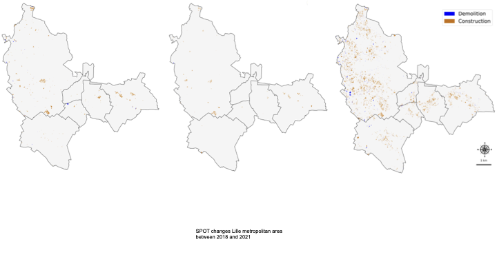
Large-scale results
In Fig. 1 of the main paper, we present large-scale results over the
metropolitan area of Lille, France (approximately 55.3 km2,
see Fig. 5 for location on France map). This
section provides additional details on the inference setup and extends
the analysis to SPOT-6/7 satellite imagery.
The large-scale inference on Lille uses BD ORTHO bi-temporal aerial
images from 2018 and 2021. We extract $`512 \times 512`$ crops with a
6-pixel overlap and feed them to our model pre-trained on b-FLAIR, as
well as to the FSC-180K model of Benidir et al. . A $`5 \times 5`$
spatial median filter is applied to the model outputs.
Motivated by the strong performance on very high-resolution aerial data,
we also evaluate our method at scale on more widely accessible satellite
imagery. We extract $`64 \times 64`$ SPOT-6/7 crops from IGN’s ORTHO-SAT
database at 1.5 m/pixel resolution with a 5% overlap. We process these
crops with the same inference pipeline and report results for both our
b-FLAIR-spot model and its STAR counterpart in
Fig. 11. As shown, the STAR model
produces many false positives, similar to FSC-180K on the BD ORTHO
experiment. In contrast, our model is substantially more robust to false
alarms and successfully highlights most large change regions, although
it remains more susceptible to false negatives.
In-domain
Out-of-Domain
3-6(lr)7-12
Filtered
Samples
b-FLAIR
b-FLAIR-spot
LEVIR-CD
WHU-CD
S2Looking
3-4(lr)5-6(lr)7-8(lr)9-10(lr)11-12
F1
IoU
F1
IoU
F1
IoU
F1
IoU
F1
IoU
b-FLAIR
Iteration 1
0
67.3
50.7
—
—
5.2
2.7
51.8
34.9
10.5
5.6
Iteration 2
484
78.1
64.1
—
—
20.3
11.3
76.1
61.4
15.4
8.3
Iteration 3
842
79.0
65.2
—
—
17.8
9.3
77.3
63.0
13.6
7.3
b-FLAIR-spot
Iteration 1
0
—
—
22.6
12.7
34.3
20.7
48.6
32.1
6.9
3.2
Iteration 2
148
—
—
21.7
12.2
35.4
21.5
47.2
30.9
5.5
2.8
Iteration 3
287
—
—
22.9
12.9
34.11
20.6
49.3
32.7
7.1
3.7
b-IAILD
Iteration 1
0
—
—
—
—
57.2
40.1
66.9
50.2
14.5
7.8
Iteration 2
49
—
—
—
—
34.4
20.8
67.9
51.4
14.7
8.0
Iteration 3
41
—
—
—
—
35.9
21.9
63.3
46.3
17.6
9.6
wl0.33wl0.33l Ground truth
& Ours & STAR
Large-scale SPOT-6/7 change detection
results. Comparison between ground truth, our b-FLAIR-SPOT
model, and the STAR approach over the metropolitan region region of
Lille, France. While our model predicts a considerable number of false
negatives, it detects most areas where larger changes were produced,
while the STAR version detects an overwhelming amount of false
positives.
Additional qualitative results
Tab. [tab:comparison_results_supp_mat]
provides additional FPR results for all evaluated methods as an
extension of the results presented in the main paper. Our method
consistently leads to less false positive than baselines, though
performing on par with them w.r.t other metrics on most datasets. This
is especially the case on in-domain datasets and on WHU-CD. In
Fig. 12, we can clearly see
that, on b-FLAIR-test-spot, our method mostly predict no change, whereas
its change predictions are accurate (see first row). On the contrary,
the other methods show a significant number of false alarms, making them
unusable in practical applications. This behavior can also be observed
with the zero-shot qualitative results on LEVIR-CD
(Fig. 13) and WHU-CD
(Fig. 14). On S2Looking
(Fig. 15), all methods globally
perform poorly due to the important domain gap with the training data.
Detailed impact of the iterative refinement
Tab. [tab:iteration_comparison_bflairspot_full]
reports the results for each iteration of our models trained on b-FLAIR,
b-FLAIR-spot, and b-IAILD, respectively. Although we set the
hyperparameter $`N_\text{iter}=3`$ based solely on in-domain dataset
results, we also report the impact of iterative refinement on
out-of-domain zero-shot performance. With the exception of the b-IAILD
model on LEVIR-CD, where the first iteration significantly outperforms
subsequent ones, removing detected change pairs from the dataset
generally benefits out-of-domain performance. The number of filtered
pairs at each iteration suggests that additional iterations could
further improve model performance. However, given the marginal
improvement between the second and third iterations on in-domain
evaluation and considering computational cost constraints, we did not
explore values of $`N_\text{iter}`$ greater than 3.
Image It
Image It′
Ground truth
Post-classif.
Post-classif.
STAR
Ours
+ temporal aug.
Qualitative results on b-FLAIR-spot-test.
We compare the building change maps predicted by baseline methods and
ours.
Qualitative zero-shot results on LEVIR-CD
for 3 randomly selected input pairs. “PC” stands for
“post-classification” and “p.t.” for “pre-training”.Qualitative zero-shot results on WHU-CD for
3 randomly selected input pairs. “PC” stands for “post-classification”
and “p.t.” for “pre-training”.Qualitative zero-shot results on S2Looking
for 3 randomly selected input pairs. “PC” stands for
“post-classification” and “p.t.” for “pre-training”.
The copyright of this content belongs to the respective researchers. We deeply appreciate their hard work and contribution to the advancement of human civilization.