Routing by Analogy kNN-Augmented Expert Assignment for Mixture-of-Experts
📝 Original Paper Info
- Title: Routing by Analogy kNN-Augmented Expert Assignment for Mixture-of-Experts- ArXiv ID: 2601.02144
- Date: 2026-01-05
- Authors: Boxuan Lyu, Soichiro Murakami, Hidetaka Kamigaito, Peinan Zhang
📝 Abstract
Mixture-of-Experts (MoE) architectures scale large language models efficiently by employing a parametric "router" to dispatch tokens to a sparse subset of experts. Typically, this router is trained once and then frozen, rendering routing decisions brittle under distribution shifts. We address this limitation by introducing kNN-MoE, a retrieval-augmented routing framework that reuses optimal expert assignments from a memory of similar past cases. This memory is constructed offline by directly optimizing token-wise routing logits to maximize the likelihood on a reference set. Crucially, we use the aggregate similarity of retrieved neighbors as a confidence-driven mixing coefficient, thus allowing the method to fall back to the frozen router when no relevant cases are found. Experiments show kNN-MoE outperforms zero-shot baselines and rivals computationally expensive supervised fine-tuning.💡 Summary & Analysis
1. **Key Contribution 1: Development of kNN-MoE** Traditional models use a static router to select expert nodes, which lacks flexibility when dealing with new inputs. The kNN-MoE overcomes this by retrieving and using optimally assigned experts from memory. This is like an autonomous car using past route data to navigate new paths.-
Key Contribution 2: Confidence-Aware Adaptive Mixing
kNN-MoE retrieves the most similar past inputs to current ones and uses them to determine a new expert assignment. The similarity score used in this process is akin to weather forecasting, where past temperature patterns are leveraged when conditions are similar. -
Key Contribution 3: Performance Improvement with Efficiency
kNN-MoE improves performance without modifying the model’s parameters, which can be likened to adding new features to software without needing an update.
📄 Full Paper Content (ArXiv Source)
 style="width:100.0%" />
The scaling of Large Language Models (LLMs) has been significantly advanced by combining Transformers with Mixture-of-Experts (MoE) architectures , which increase model capacity via sparse activation without a proportional increase in computational cost . A routing network (or “router”) dynamically activates a small subset of experts for each input token . However, the efficacy of an MoE model hinges critically on the quality of its routing decisions.
Standard routers are lightweight, parametric classifiers trained to predict expert assignments based on hidden states. Once trained, the router implements a fixed policy. While effective on in-distribution data, it lacks the flexibility to adjust routing decisions during inference. When facing inputs that deviate from the training distribution—often manifested as high perplexity—the router must extrapolate from fixed priors, potentially selecting suboptimal experts . This lack of flexibility restricts the potential of MoE models, particularly on specialized or out-of-distribution tasks.
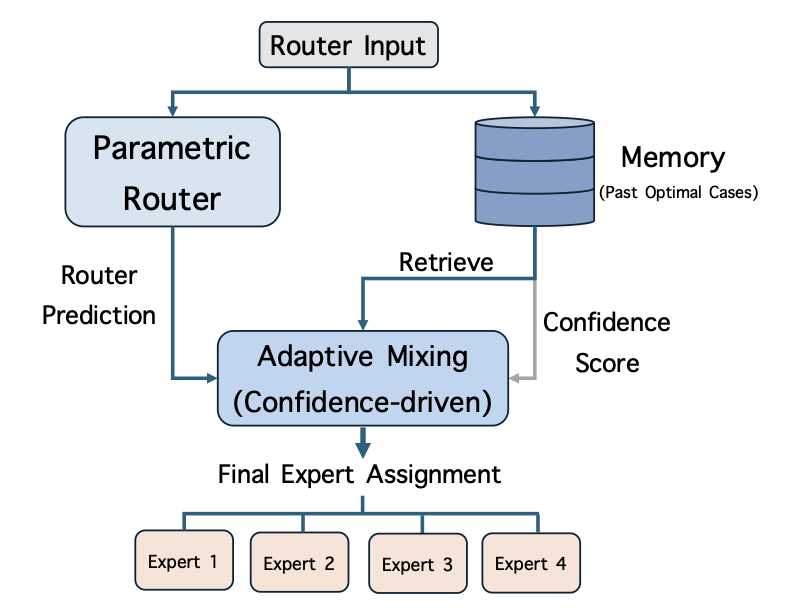
In this paper, we propose kNN-MoE, which refines routing decisions by retrieving the nearest neighbors of past router inputs and reusing their offline-computed optimal expert assignments (Figure 1). Concretely, we build a memory that stores router inputs (keys) paired with optimal expert assignments (values) obtained by maximizing the likelihood on a reference set. At test time, kNN-MoE retrieves similar keys from the memory whose expert assignments led to higher past case likelihoods and then interpolates the router prediction with the retrieved expert assignment, using similarity as a confidence score. Intuitively, when retrieved neighbors are highly similar, the method trusts the retrieved routing; otherwise, it falls back to the original parametric router, avoiding noise from irrelevant retrievals.
We evaluated kNN-MoE on three MoE models—OLMoE , GPT-OSS , and Qwen3 —across benchmarks including GPQA , SuperGPQA , MMLU , and medical tasks (USMLE and MedMCQA ). Empirical results show that kNN-MoE outperforms zero-shot baselines and achieves performance competitive with computationally intensive supervised fine-tuning, all without modifying the model parameters. Ultimately, kNN-MoE bridges the gap between static parametric routing and dynamic inference needs, offering a scalable pathway to enhance MoE adaptability without the computational burden of fine-tuning.
Related Work
Expert Assignment Optimization for MoE
Optimizing expert assignments in MoE has been demonstrated by prior work to enhance model performance. For instance, proposed C3PO, a test-time adaptation method that fine-tunes routing logits using examples correctly answered by the model; however, this approach incurs a computational cost approximately five times higher than that of the baseline .
Additionally, concurrent work includes , who proposed fine-tuning the router with an auxiliary loss. Unlike our non-parametric approach which keeps the model frozen, their method relies on permanently updating the router parameters. Similarly, proposed a test-time adaptation framework that optimizes expert assignment on-the-fly by minimizing self-supervised loss on the input context. In contrast, our framework avoids online optimization overhead by directly retrieving cached optimal assignments from a memory store.
Non-Parametric and Retrieval-Augmented LMs
Our work is closely related to non-parametric methods that augment neural networks with external data stores. A prominent line of research involves kNN-LMs , which retrieve nearest neighbor tokens from a data store of cached hidden states to interpolate the final output distribution. Similarly, Retrieval-Augmented Generation models retrieve textual chunks to condition the generation process. Furthermore, explored retrieving past high-utility decisions in reranking to guide output selection.
Mixture-of-Experts
Consider an MoE Transformer model with $`L`$ layers, where a subset of indices $`\mathcal{L}_{\text{MoE}} \subset \{1, \dots, L\}`$ corresponds to layers. For any specific layer $`\ell \in \mathcal{L}_{\text{MoE}}`$, the module consists of $`N`$ expert networks $`\{E^{(\ell)}_i\}_{i=1}^N`$ and a router $`R^{(\ell)}`$.
Let $`x^{(\ell)} \in \mathbb{R}^d`$ denote the input hidden state of the MoE module at layer $`\ell`$, which is typically the output of the preceding attention block or normalization module. The core mechanism of the MoE module employs a router to assign the input to the most relevant experts. The router is typically parameterized by a learnable weight matrix $`W_r^{(\ell)} \in \mathbb{R}^{d \times N}`$, and it generates the expert assignment (a sparse gating distribution) $`a^{(\ell)}(x^{(\ell)}) \in \mathbb{R}^N`$ via a Top-$`k`$ softmax function:
\begin{equation}
    \label{eq:router_gate}
    a^{(\ell)}(x^{(\ell)}) = \mathrm{TopK}\left(\mathrm{Softmax}(x^{(\ell)} W_r^{(\ell)})\right).
\end{equation}The final output of the MoE module, denoted as $`h^{(\ell)}`$, is computed as the linear combination of the selected experts’ outputs using the predicted expert assignment:
\begin{equation}
    \label{eq:moe_output}
    h^{(\ell)} = \sum_{i=1}^N a^{(\ell)}(x^{(\ell)})_i \cdot E^{(\ell)}_i(x^{(\ell)}).\nonumber
\end{equation}During standard inference, the router weights $`W_r^{(\ell)}`$ remain fixed. This static routing strategy may limit adaptability when the test distribution diverges from the training distribution.
Proposed Method: kNN-MoE
We propose kNN-MoE (Figure 1), a retrieval-based framework that enhances routing decisions by leveraging a memory of historical router inputs and their optimal expert assignments. We equip each MoE module $`\ell \in \mathcal{L}_{\text{MoE}}`$ with an independent memory store $`\mathcal{M}^{(\ell)}`$. We omit the layer superscript $`(\ell)`$ as the method operates identically across layers. kNN-MoE consists of two phases: (1) Memory Construction (§4.1), which builds the expert assignment memory offline; and (2) Confidence-Aware Adaptive Mixing (§4.2), which retrieves and utilizes stored expert assignments during inference.
Memory Construction
The goal of memory construction is to create a key-value store $`\mathcal{M} = \{(k_t, v_t)\}`$ for the layer, where the key $`k_t`$ is a router input and the value $`v_t`$ is the optimal expert assignment that outperforms the original router. This process involves two steps: data collection and deriving optimal expert assignments.
Data Collection
We use a reference dataset $`\mathcal{D}_{\text{ref}}`$ consisting of sequences of ground-truth tokens. Let $`\mathbf{y} = (y_1, \dots, y_T)`$ denote a sequence in $`\mathcal{D}_{\text{ref}}`$. We run the frozen MoE model on these sequences in teacher-forcing mode. For every time step $`t \in [1,T]`$, we collect the router input $`x_t`$ at the current layer and the corresponding target token $`y_t`$ from the sequence. The router input serves as the retrieval key, i.e., $`k_t = x_t`$.
Deriving Optimal Expert Assignments
Instead of storing the model’s original routing decision defined in Eq. [eq:router_gate], we seek the optimal expert assignment that maximizes the prediction probability of the ground-truth token $`y_t`$. We formulate this as an optimization problem for each token.
Let $`\pi(r) = \mathrm{TopK}(\mathrm{Softmax}(r))`$ denote the mapping from logits $`r \in \mathbb{R}^N`$ to sparse expert weights. For a specific token $`t`$, we introduce a learnable logit vector $`r_t`$ to replace the parametric output $`x_t W_r`$. We optimize $`r_t`$ to minimize the negative log-likelihood of the target token $`y_t`$:
\begin{align}
    \label{eq:gold_routing_obj}
    r_t^{*} &= \mathop{\rm arg~min}\limits_{r \in \mathbb{R}^N} \mathcal{L}_t(r), \\
    \mathcal{L}_t(r) &= - \log p_\theta\bigl(y_t \mid x_t, \text{routing}{=}\pi(r)\bigr), \nonumber
\end{align}where $`\theta`$ represents the frozen parameters of the rest of the network.
We solve Eq. [eq:gold_routing_obj] via gradient descent. We initialize $`r_t`$ with the original parametric logits, i.e., $`r_t^{(0)} = x_t W_r`$. We then perform $`S`$ steps of updates:
\begin{equation}
    r_t^{(s+1)} = r_t^{(s)} - \eta \nabla_r \mathcal{L}_t(r_t^{(s)}), ~~ \text{for } s = 0, \dots, S-1,\nonumber
\end{equation}where $`\eta`$ is the learning rate. Note that while we describe $`r_t`$ for a generic layer, this optimization is performed jointly across the entire model; specifically, the routing logits of all layers $`\{r_t^{(\ell)}\}_{\ell \in \mathcal{L}_{\text{MoE}}}`$ are updated simultaneously to minimize the loss. Additionally, the optimization and data collection processes are conducted independently across different sequences in $`\mathcal{D}_{\text{ref}}`$.
The final optimized assignment is $`a^*(x_t) = \pi(r_t^{(S)})`$. This value serves as the target value in our memory, $`v_t = a^*(x_t)`$. It represents the “optimal” choice: which experts should have been selected to best predict the next token.
Finally, the memory for the current layer is constructed as:
\begin{equation}
    \mathcal{M} = \{(x_t, a^*(x_t)) \mid t \in \mathcal{D}_{\text{ref}}\}.\nonumber
\end{equation}This process is repeated for every layer in $`\mathcal{L}_{\text{MoE}}`$.
Confidence-Aware Adaptive Mixing
During inference, for each MoE layer and each router input $`x`$, we retrieve the set of $`K`$ nearest neighbors $`\mathcal{N}(x) \subset \mathcal{M}`$ from the corresponding memory constructed in §4.1.
We formulate a non-parametric expert assignment proposal, denoted as $`a_{\text{mem}}(x)`$, by aggregating the retrieved expert assignments according to their similarity to the input. Specifically, let $`\{(k_j, v_j)\}_{j=1}^K`$ be the retrieved key-value pairs in $`\mathcal{N}(x)`$. The memory-based expert assignment is computed as:
\begin{equation}
    \label{eq:mem_gate}
    a_{\text{mem}}(x) = \sum_{j=1}^K \frac{s(x, k_j)}{\sum_{m=1}^K s(x, k_m)} \, v_j,\nonumber
\end{equation}where $`s(\cdot, \cdot)`$ is a similarity function.
To fuse the parametric router output $`a(x)`$ (as defined in Eq. [eq:router_gate]) with the non-parametric proposal $`a_{\text{mem}}(x)`$, we introduce an adaptive mixing coefficient $`\lambda(x)`$ that reflects retrieval confidence. We quantify this confidence using the average similarity of the neighbors:
\begin{equation}
    \lambda(x) = \frac{1}{K} \sum_{j=1}^K s(x, k_j).\nonumber
\end{equation}The final expert assignment is obtained by linearly interpolating between the parametric and memory-based assignments:
\begin{equation}
    \label{eq:final_gating}
    a_{\text{final}}(x) = (1 - \lambda(x)) a(x) + \lambda(x) a_{\text{mem}}(x).\nonumber
\end{equation}Finally, we use $`a_{\text{final}}(x)`$ to compute the MoE layer output $`h`$:
\begin{equation}
    h = \sum_{i=1}^N a_{\text{final}}(x)_i \cdot E_i(x).\nonumber
\end{equation}This mixing ensures that when $`\lambda(x) \approx 1`$, the model trusts the retrieved assignment to correct the router; conversely, when $`\lambda(x) \approx 0`$, it falls back to the parametric router to avoid retrieval noise.
| Benchmark | Test Source | Ref. Source | $`|\mathcal{D}_{\text{test}}|`$ | $`|\mathcal{D}_{\text{ref}}|`$ | |:—|:–:|:–:|:–:|:–:| | GPQA | GPQA Diamond | GPQA Main (filtered) | $`0.20`$k | $`0.20`$k | | MMLU | Test subset | Train subset | $`14.00`$k | $`1.81`$k | | SuperGPQA | Held-out split | Random subset | $`23.50`$k | $`3.00`$k | | USMLE | Test subset | Train subset | $`1.27`$k | $`0.20`$k | | MedMCQA | Test subset | Train subset | $`6.15`$k | $`1.00`$k |
Experiments
Experimental Settings
| Model | Method | GPQA | MMLU | SuperGPQA | USMLE | MedMCQA |
|---|---|---|---|---|---|---|
| OLMoE | Zero-shot | 27.27 | 46.77 | 13.02 | 32.81 | 35.57 |
| 5-shot | 21.72 | 33.06 | 11.09 | 31.31 | 25.36 | |
| SFT | 21.72 | 46.89 | 13.67 | 37.84 | 34.78 | |
| SFT (Router Only) | 24.24 | 45.27 | 11.66 | 31.22 | 34.23 | |
| kNN-MoE (Ours) | 29.80 | 47.81 | 13.27 | 35.04 | 37.01 | |
| GPT-OSS | Zero-shot | 43.94 | 70.20 | 23.52 | 67.29 | 56.20 |
| 5-shot | 36.87 | 63.72 | 19.95 | 60.02 | 52.76 | |
| SFT | 41.92 | 70.28 | 24.83 | 65.61 | 56.06 | |
| SFT (Router Only) | 41.41 | 69.18 | 18.83 | 65.05 | 54.89 | |
| kNN-MoE (Ours) | 45.45 | 70.28 | 24.35 | 68.31 | 57.06 | |
| Qwen3 | Zero-shot | 41.41 | 78.59 | 34.85 | 75.30 | 62.51 |
| 5-shot | 44.44 | 80.48 | 35.56 | 77.17 | 66.58 | |
| SFT | 39.90 | 79.08 | 40.20 | 80.80 | 66.60 | |
| SFT (Router Only) | 43.94 | 78.36 | 33.15 | 76.05 | 66.03 | |
| kNN-MoE (Ours) | 44.95 | 78.86 | 35.15 | 76.70 | 66.65 |
Datasets
We evaluated kNN-MoE on general reasoning and domain-specific benchmarks: GPQA, SuperGPQA, MMLU, USMLE, and MedMCQA. For each, we defined a disjoint test set $`\mathcal{D}_{\text{test}}`$ and a reference set $`\mathcal{D}_{\text{ref}}`$. The same $`\mathcal{D}_{\text{ref}}`$ was reused across all methods: kNN-MoE used it to construct the expert assignment memory, 5-shot used it as the retrieval pool for in-context examples, and supervised fine-tuning (SFT) used it as the training dataset. Table [tab:data_stats] detailed the splits.
Models
We employed three representative MoE models: OLMoE
(allenai/OLMoE-1B-7B-0125-Instruct) , GPT-OSS (openai/gpt-oss-20b) ,
and Qwen3 (Qwen/Qwen3-30B-A3B-Instruct-2507) . These models were
selected because they incorporated modern MoE architectural designs and
were computationally feasible to run within our research budget.
Baselines
We compared kNN-MoE against two categories of baselines. First, we included Zero-shot and 5-shot as standard, cost-effective inference baselines. Second, and importantly, we compared against SFT. Since kNN-MoE leveraged the reference set $`\mathcal{D}_{\text{ref}}`$ to improve performance, SFT served as the primary methodological baseline: similar to kNN-MoE, it utilized the reference set $`\mathcal{D}_{\text{ref}}`$ to optimize performance in an offline stage (training), ensuring that the inference process remained efficient. This made SFT the most direct comparison for evaluating the efficacy of our offline memory construction.
-
Zero-shot: Zero-shot used the original MoE model with its parametric routers $`R^{(\ell)}`$ and a zero-shot QA prompt.
-
5-shot: For each test instance in $`\mathcal{D}_{\text{test}}`$, we constructed a 5-shot prompt by retrieving five examples from the reference set $`\mathcal{D}_{\text{ref}}`$ whose input questions were most similar to the test question. Concretely, we encoded all questions using the
Qwen3-Embedding-0.6Bsentence embedding model and selected the five reference questions with the highest cosine similarity to the test question. These examples, together with their correct answers, were concatenated before the test question to form the in-context prompt. -
SFT: For SFT, we trained on $`\mathcal{D}_{\text{ref}}`$ using standard cross-entropy loss over the correct answers. We applied LoRA adapters to all linear layers. We set the maximum number of training epochs to $`3`$, split $`\mathcal{D}_{\text{ref}}`$ into an 85% training split and a 15% validation split, and selected the checkpoint with the lowest validation loss. During training and inference, SFT used a zero-shot QA prompt.
-
SFT (Router Only): We fine-tuned only the router parameters $`\{W_r^{(\ell)}\}_{\ell \in \mathcal{L}_{\text{MoE}}}`$ on $`\mathcal{D}_{\text{ref}}`$, while freezing all expert and non-router parameters. The training objective was the same supervised cross-entropy loss as in SFT. We used the same training protocol (including training epochs, data splitting, and checkpoint selection methods) and prompt as SFT.
See Appendix 8 and 9 for details on prompt templates and SFT training, respectively.
Note on Other Methods
We excluded token-level retrieval methods like kNN-LM from the main comparison due to the lack of efficient implementations compatible with modern LLM architectures. Furthermore, we deferred the comparison with C3PO to the Discussion section (§6.7). The rationale was that C3PO operated as a test-time adaptation method, performing computationally intensive optimization during inference for each input. In contrast, kNN-MoE aligned with the SFT paradigm by shifting the computational burden to an offline memory construction, allowing for fast inference. Thus, we treated C3PO as a distinct category of method with different latency-accuracy trade-offs.
Implementation Details of kNN-MoE
We used FAISS for retrieval and built one index per MoE layer, using the router inputs $`\{x_t\}`$ stored in that layer’s memory $`\mathcal{M}`$ as keys. We used a single hyperparameter $`K`$ (neighbors per router) and shared it across layers; by default, we set $`K=1`$ based on validation (§6.3). We set the learning rate to $`\eta = 2 \times 10^{-2}`$ and used a single gradient descent step ($`S=1`$) for each token. We found that using more steps (e.g., $`S=3`$ or $`S=10`$) yielded very similar performance while incurring a substantially higher construction cost; we provided an ablation over $`S`$ in §6.4. The similarity function was an RBF kernel $`s(x, k) = \exp(-\gamma \|x - k\|^2)`$, with $`\gamma`$ set heuristically based on the average nearest neighbor distance in the memory.
Evaluation
We reported accuracy (%) on $`\mathcal{D}_{\text{test}}`$ for all datasets, using the official benchmark answers. To ensure a fair comparison, we kept the answer parsing identical across all methods.
Results
Table [tab:main_results] summarizes the main results across the three MoE models. Our findings are as follows:
Comparison with Zero-shot and SFT (Router Only)
Across all models and datasets, kNN-MoE consistently improves over both Zero-shot and SFT (Router Only). These trends indicate that refining expert assignment via retrieved cases is more effective than solely relying on the fixed parametric router, even without any task-specific parameter updates during inference.
Comparison with 5-shot
Compared to 5-shot, kNN-MoE exhibits more stable behavior across models. On Qwen3 30B, both 5-shot and kNN-MoE can improve over Zero-shot; but for GPT-OSS and OLMoE, 5-shot often degrades performance relative to Zero-shot. A likely reason is that concatenating the five nearest reference examples substantially lengthens the input sequence, pushing these models into length regimes where their performance is less robust and amplifying the effect of retrieval noise.
Comparison with SFT
While kNN-MoE outperforms SFT in certain scenarios, its relative performance varies. In settings with limited reference sets (GPQA and USMLE), SFT occasionally underperforms compared to Zero-shot. We attribute this degradation to potential overfitting induced by the small dataset size. In contrast, our kNN-MoE consistently outperforms Zero-shot in these data-scarce settings.
Conclusion
Overall, we conclude that kNN-MoE provides a robust routing refinement for MoE models: it outperforms zero-shot and the router-only SFT baseline, and it is competitive with SFT.
Discussion
Why Case-Based MoE Works
Our main hypothesis is that retrieval is most beneficial when the parametric router is uncertain, which is often correlated with increased perplexity. To test this, we bucketed test instances into three equal-sized groups based on the perplexity (PPL) of the original model (with zero-shot prompt) (High / Mid / Low PPL), and reported the accuracy gain of kNN-MoE over Zero-shot baseline within each bucket. Table 1 reports results on OLMoE.
| Benchmark | High PPL | Mid PPL | Low PPL |
|---|---|---|---|
| GPQA | +6.15 | +2.99 | -1.52 |
| SuperGPQA | +0.17 | +0.65 | -0.06 |
| MMLU | +2.07 | +1.15 | -0.13 |
| USMLE | +6.32 | +1.41 | -1.13 |
| MedMCQA | +6.04 | +1.13 | +0.56 |
Accuracy gains (kNN-MoE minus Zero-shot) bucketed by perplexity (PPL) of the original model (Zero-shot), using OLMoE.
kNN-MoE usually yields the largest gains on High-PPL instances across all benchmarks (e.g., +6.15 on GPQA and +6.32 on USMLE), while the improvements on Mid-PPL instances are smaller but still consistently positive. In contrast, the gains on Low-PPL instances are close to zero and can become slightly negative on some datasets. The slight degradation on a subset of Low-PPL instances suggests that kNN-MoE can occasionally introduce noise when the router prediction is strong.
Overall, we hypothesize that the strong correlation between perplexity and kNN-MoE gains stems from the fact that higher perplexity indicates a greater deviation of the input from the router’s data distribution. Consequently, the expert assignment predicted by the router becomes unreliable, whereas kNN-MoE improves the assignment.
| Method | GPQA | MMLU | USMLE |
|---|---|---|---|
| kNN-MoE | 29.80 | 47.81 | 35.04 |
| kNN-MoE (Selective) | 30.30 | 47.85 | 35.41 |
Performance comparison on OLMoE between standard kNN-MoE and a Selective variant. The Selective variant falls back to the zero-shot baseline for inputs in the lowest perplexity tercile.
Inspired by this observation, we investigated a variant termed kNN-MoE (Selective). This variant dynamically deactivates retrieval for inputs where the Zero-shot baseline is confident (specifically, the bottom 33% of test instances by perplexity) and falls back to the parametric router. As shown in Table 2, this strategy yields marginal improvements (e.g., +0.50% on GPQA). However, it introduces significant computational overhead, as it requires a preliminary forward pass to estimate baseline perplexity. Given the negligible performance gain relative to the added cost, we retained the standard kNN-MoE as our primary approach.
Impact of Reference Set Size $`|\mathcal{D}_{\text{ref}}|`$
| $`|\mathcal{D}_{\text{ref}}|`$ | OLMoE | GPT-OSS | Qwen3 | |:——————————-|:—–:|:——-:|:—–:| | $`0`$ | 35.57 | 56.20 | 62.51 | | $`0.25`$k | 35.99 | 56.41 | 66.01 | | $`0.50`$k | 36.87 | 56.92 | 66.68 | | $`1.00`$k | 37.01 | 57.06 | 66.65 |
Accuracy (%) of kNN-MoE on MedMCQA as a function of the reference set size $`|\mathcal{D}_{\text{ref}}|`$ used for memory construction. $`|\mathcal{D}_{\text{ref}}|=0`$ corresponds to Zero-shot (no memory).
We next varied the size of the reference set used to build the per-layer memory and evaluate kNN-MoE on MedMCQA. Table 3 shows that larger memories generally improve performance for all three models. When $`|\mathcal{D}_{\text{ref}}|=0`$, kNN-MoE degenerates to the zero-shot baseline. As $`|\mathcal{D}_{\text{ref}}|`$ increases, accuracy improves monotonically, with diminishing returns beyond roughly $`0.5`$k–$`1`$k examples.
Impact of the Number of Neighbors ($`K`$)
| $`K`$ | OLMoE | GPT-OSS | Qwen3 |
|---|---|---|---|
| $`1`$ | 37.01 | 57.06 | 66.65 |
| $`3`$ | 36.89 | 56.55 | 65.76 |
| $`5`$ | 36.02 | 56.74 | 65.98 |
| $`10`$ | 36.34 | 56.11 | 65.19 |
Accuracy (%) of kNN-MoE on MedMCQA using different numbers of neighbors $`K`$.
We investigated the sensitivity of kNN-MoE to the value of $`K`$. Table 4 presents the accuracy on MedMCQA for varying $`K \in \{1, 3, 5, 10\}`$. Contrary to typical non-parametric approaches where aggregating multiple neighbors (e.g., $`K \ge 5`$) helps reduce variance and smooth out noise, we observe that performance consistently peaks at $`K=1`$ across all three models. As $`K`$ increases, accuracy generally degrades.
We interpret this essentially as a negative result regarding the benefit of neighbor aggregation in the context of MoE routing. This phenomenon suggests that the optimal expert assignments responsible for positive outcomes are rare within the memory $`\mathcal{M}`$. In other words, for a given query, there is often only a single (or very few) historical case that provides a truly beneficial routing signal. Consequently, forcing the retrieval of additional neighbors ($`K > 1`$) likely incorporates cases with lower relevance or conflicting expert assignments. Instead of reinforcing the correct decision, these additional neighbors dilute the strong signal provided by the nearest neighbor, thereby introducing noise that harms the final model performance. Based on this finding, we adopt $`K=1`$ as the default setting for all other experiments.
Impact of Gradient Descent Steps ($`S`$)
| $`S`$ | OLMoE | GPT-OSS | Qwen3 |
|---|---|---|---|
| $`1`$ | 37.01 | 57.06 | 66.65 |
| $`3`$ | 37.05 | 57.12 | 66.58 |
| $`10`$ | 36.98 | 57.01 | 66.71 |
Accuracy (%) of kNN-MoE on MedMCQA with varying gradient descent steps $`S`$ used for memory construction.
We studied the impact of the number of gradient descent steps $`S`$ used during the Memory Construction phase (§4.1) to derive the optimal expert assignment. Intuitively, more optimization steps should lead to a lower negative log-likelihood on the reference tokens, potentially yielding higher-quality targets for the memory. We compared the performance of kNN-MoE constructed with $`S \in \{1, 3, 10\}`$ steps.
Table 5 summarizes the results on MedMCQA. We observe that increasing $`S`$ beyond a single step yields negligible improvements in downstream accuracy. We hypothesize that the initial gradient direction $`\nabla_r \mathcal{L}_t(r_t^{(0)})`$ already captures the most critical information regarding which experts are under-utilized or should be promoted. Since the memory stores discrete optimal assignment values $`v_t`$, slight refinements to the logits $`r_t`$ in subsequent steps ($`S>1`$) may not significantly alter the top-k ranking or the resulting routing distribution used as targets. Crucially, the computational cost of memory construction scales linearly with $`S`$. Setting $`S=1`$ allows for rapid memory construction (as shown in §6.6) without compromising model performance. Therefore, we adopted $`S=1`$ as the default setting for efficiency.
Impact of Choice of $`s(\cdot, \cdot)`$
| $`s(\cdot, \cdot)`$ | OLMoE | GPT-OSS | Qwen3 |
|---|---|---|---|
| RBF | 37.01 | 57.06 | 66.65 |
| Cosine | 36.69 | 56.01 | 66.65 |
Accuracy (%) of kNN-MoE on MedMCQA using different similarity functions $`s(\cdot, \cdot)`$.
We analyzed the sensitivity of kNN-MoE to the choice of the similarity function $`s(x, x')`$. Specifically, we compared our default RBF kernel, which relies on Euclidean distance, against cosine similarity, which measures the cosine of the angle between vectors. Table 6 presents the results on MedMCQA. We observe that the RBF kernel outperforms or matches cosine similarity.
We conjecture that this disparity stems from the way each metric handles vector magnitude. Cosine similarity normalizes the input vectors, effectively projecting them onto a unit hypersphere and discarding the information encoded in their norms: $`s_{\text{cosine}}(x, k) = \frac{x \cdot k}{\|x\| \|k\|}`$. In contrast, the RBF kernel depends on the distance $`\|x - k\|^2`$, which inherently preserves information about the scale (magnitude) of the router inputs. The superior performance of RBF on OLMoE and GPT-OSS suggests that for these architectures, the magnitude of the router input vector $`x`$ likely exhibits significant variance and carries discriminative signals for expert assignment—information that is discarded when using cosine similarity. Conversely, the insensitivity of Qwen3 to the results with different metrics imply that its router inputs may be more uniform in magnitude or that its routing policy is primarily direction-dependent.
Memory Construction and Inference Costs
We investigated the memory construction and inference costs of kNN-MoE. Table 7 compares the preparation time on OLMoE with $`|\mathcal{D}_{\text{ref}}|=1.00`$k, all conducted on a single NVIDIA A100 80GB. Constructing the kNN-MoE memory took 0.46 hours, which was substantially faster than both SFT and SFT (Router Only). This speedup is mainly driven by optimizing token-specific routing logits (rather than updating model parameters) and using only one gradient descent step per token.
| $`|\mathcal{D}_{\text{ref}}|`$ | SFT | SFT (Router Only) | kNN-MoE | |:——————————-|:—–:|:—————–:|:——-:| | $`1.00`$k | 1.34h | 1.33h | 0.46h |
Memory construction time on OLMoE with $`|\mathcal{D}_{\text{ref}}|=1`$k. Other reference sizes scale approximately linearly with $`|\mathcal{D}_{\text{ref}}|`$.
At inference time, kNN-MoE incurs additional latency due to per-token nearest neighbor retrieval. Table 8 reports the average latency per example as a function of $`|\mathcal{D}_{\text{ref}}|`$. As expected, latency increases with $`|\mathcal{D}_{\text{ref}}|`$ because each router query searches a larger index. With $`|\mathcal{D}_{\text{ref}}|=1.00`$k and $`K=1`$, the overhead remains moderate (e.g., OLMoE increases from 1.27s to 1.70s per example). These results motivate future directions that reduce retrieval cost via memory pruning or compression.
| $`|\mathcal{D}_{\text{ref}}|`$ | OLMoE | GPT-OSS | Qwen3 | |:——————————-|:—–:|:——-:|:—–:| | $`0`$ | 1.27s | 2.32s | 5.99s | | $`0.25`$k | 1.33s | 2.44s | 6.19s | | $`0.50`$k | 1.54s | 2.51s | 6.41s | | $`1.00`$k | 1.70s | 2.98s | 6.83s |
Inference speed (seconds per example) using different reference set sizes $`|\mathcal{D}_{\text{ref}}|`$.
Comparison with C3PO
| Method | GPQA | MMLU | USMLE |
|---|---|---|---|
| Zero-shot | 27.27 | 46.77 | 32.81 |
| C3PO | 24.24 | 48.04 | 32.93 |
| kNN-MoE | 29.80 | 47.81 | 35.04 |
Performance comparison with the state-of-the-art method C3PO using the OLMoE model. kNN-MoE demonstrates superior sample efficiency on smaller datasets (GPQA, USMLE).
We compared kNN-MoE with C3PO , a state-of-the-art test-time routing adaptation method. Table 9 presents the accuracy on OLMoE across three benchmarks with varying reference set sizes. We observe distinct behaviors depending on the availability of reference data. On benchmarks with limited reference sets, (GPQA and USMLE), C3PO yields marginal gains or even performance degradation compared to the zero-shot baseline. In contrast, kNN-MoE achieves consistent improvements in these data-scarce regimes. However, on MMLU, which provides a larger reference set ($`|\mathcal{D}_{\text{ref}}| \approx 1.81`$k), C3PO outperforms kNN-MoE.
We attribute these findings to the difference in sample efficiency. C3PO relies on a filtering mechanism that only utilizes reference examples correctly predicted by the baseline model to guide the router update. This significantly reduces the effective training signal when the reference set is small or the task is difficult. Conversely, kNN-MoE exploits all retrieved neighbors by computing the optimal expert assignment that maximizes the likelihood of the ground-truth token, regardless of the original model’s correctness. This capability allows kNN-MoE to extract richer supervision signals from small datasets, making it more robust for specialized domains with limited data.
Conclusions and Future Work
We introduced kNN-MoE, a routing framework that augments each parametric router in an MoE model with a non-parametric memory of optimal expert assignments derived offline from a labeled reference set. By retrieving nearest neighbors in the space of router inputs and interpolating their expert assignments with the router prediction using a similarity-based confidence coefficient, kNN-MoE improves routing decisions without updating model parameters. Across three MoE models and five challenging benchmarks, kNN-MoE consistently outperforms Zero-shot and router-only SFT, and it is competitive with SFT while requiring substantially less preparation time.
There are several promising directions for future work. First, we will investigate accelerating retrieval by pruning the memory or compressing the stored router inputs (keys), for example, by reducing the vector dimensionality or applying quantization, aiming to reduce index size and distance computation while preserving accuracy. Second, we will extend kNN-MoE to settings where the reference set is unlabeled: we can use LLM-as-a-judge to generate pseudo labels on the reference set, and then apply the same likelihood maximization procedure to construct optimal expert assignments from these pseudo labels.
Limitations
The primary limitation of our current framework lies in its dependence on a labeled reference set ($`\mathcal{D}_{\text{ref}}`$) that shares a similar distribution with the target test data. Our experimental success is predicated on the assumption that such accessible, high-quality data is available. However, in practical, open-ended deployment scenarios, acquiring domain-specific labeled data can be challenging or expensive. Consequently, this dependency may restrict the applicability of kNN-MoE in strictly zero-resource settings or when facing severe distribution shifts where no relevant historical cases exist. As mentioned in Section 7, leveraging “LLM-as-a-judge” to generate pseudo-labels offers a potential pathway to mitigate this constraint by utilizing unlabeled data; however, we leave the validation of this semi-supervised approach to future work.
Additionally, while kNN-MoE avoids the high cost of parameter updates, the non-parametric retrieval mechanism introduces necessary overheads. Specifically, the inference latency increases due to neighbor search (as shown in Table 8), and the memory storage requirements scale linearly with the size of the reference set. While currently manageable for the scales investigated in this paper, these factors may necessitate further optimization, such as memory quantization or index pruning, for deployment in strictly resource-constrained environments.
Prompt Templates
To ensure reproducibility, we provide the exact prompt templates used for our Zero-shot and 5-shot inference baselines. Please note that the templates below illustrate the case for multiple-choice questions with four options (A–D). For questions with a different number of options, the list of choices is adjusted accordingly while maintaining the same overall format.
Zero-shot Prompt
For all models and test sets in the Zero-shot setting, we formatted the
input question and options using the template below. The placeholders
{question} and {choices} are substituted with the specific instance
data.
What is the correct answer to this question: {question}
Choices:
(A) {choices[0]}
(B) {choices[1]}
(C) {choices[2]}
(D) {choices[3]}
Answer with the format: The correct answer is (X).
5-shot Prompt
For the 5-shot setting, we constructed the prompt by concatenating five retrieved expert examples followed by the target question. Similar to the zero-shot case, the example below assumes four choices per question.
Here are some example expert multiple-choice questions. After the examples, answer the final question.
Question: {s1.question}
Choices:
(A) {s1.choices[0]}
(B) {s1.choices[1]}
(C) {s1.choices[2]}
(D) {s1.choices[3]}
The correct answer is ({s1.answer})
… [3 more examples] …
Question: {s5.question}
Choices:
(A) {s5.choices[0]}
(B) {s5.choices[1]}
(C) {s5.choices[2]}
(D) {s5.choices[3]}
The correct answer is ({s5.answer})
Question: {target.question}
Choices:
(A) {target.choices[0]}
(B) {target.choices[1]}
(C) {target.choices[2]}
(D) {target.choices[3]}
Training Implementation Details
Our supervised fine-tuning baselines—SFT and SFT (Router Only)—were implemented based on the TRL library1. In the SFT (Router Only) setting, we constrained the optimizer to update only the router parameters.
Table [tab:hyperparams] summarizes the hyperparameters used for training.
| Configuration | Value |
|---|---|
| Optimization | |
| Optimizer | AdamW |
| Batch Size | 16 |
| Weight Decay | 0.01 |
| Learning Rate Schedule | Linear Decay |
| LoRA Parameters | |
| Rank (r) | 32 |
| Alpha (α) | 32 |
| Dropout | 0.0 |
| Bias | None |
| Hardware | |
| GPU | 1 × NVIDIA A100 (80GB) |
📊 논문 시각자료 (Figures)