Robust and Efficient Zeroth-Order LLM Fine-Tuning via Adaptive Bayesian Subspace Optimizer

Several strategies have been proposed to reduce memory burden. Parameter-efficient fine-tuning (PEFT) methods, including LoRA (Hu et al., 2022) and Adapters (Houlsby et al., 2019), freeze the base model and only update a small set of additional parameters. But these methods still rely on backpropagation and may underperform full fine-tuning on difficult tasks. An alternative direction is zeroth-order (ZO) optimization, which estimates gradients using only forward passes. MeZO (Malladi et al., 2023) demonstrated that this approach can match the memory footprint of inference, while achieving reasonable accuracy. The catch? ZO methods converge slowly and require significantly more iterations than their first-order counterparts, due to the high variance inherent in finite-difference gradient estimates. This raises a question: how can we achieve a better tradeoff between convergence speed and memory usage? We observe that the existing ZO methods have three main weaknesses. First, most existing ZO optimizers essentially perform updates along a single random direction within each batch. Even with increased forward passes and perturbation directions, they process each perturbation in isolation, simply averaging or using them independently-throwing away information about how these measurements relate to each other. Second, the noise level in ZO estimates varies significantly during training, yet most methods do not account for this effect. This rigidity leads to poor adaptation: updates may oscillate wildly around local minima, jump out of the basin, and finally cause training collapse. Moreover, reduced-precision training (fp16/bf16) can cause these methods to collapse or suffer substantial performance degradation, as we show in Figure 1 and Table 3.

We propose Bayesian Subspace Zeroth-order Optimization (BSZO) to address these limitations. The main idea is to treat gradient estimation as an inference problem. At each step, we sample k random directions to form a lowdimensional subspace (Zhang, 2025) and model the projected gradient as a latent variable. Instead of treating each finite-difference query as providing an independent estimate, we use Kalman filtering to aggregate observations-essentially asking: given what we have measured so far, what is our best guess of the true gradient? This Bayesian formulation accounts for measurement noise and produces more accurate estimates from the same number of forward passes. We further introduce an adaptive mechanism that tracks prediction residuals and adjusts the noise variance on the fly, allowing the algorithm to respond to changing curvature conditions during training.

Our contributions can be summarized as follows:

1. We propose BSZO, a zeroth-order optimizer that uses Bayesian inference to aggregate gradient information across multiple perturbation directions within a subspace. To our knowledge, this is the first application of Bayesian inference and Kalman filtering to ZO optimization for LLMs.

2. We design a residual-based adaptive scheme that enables BSZO to adjust the parameter update scale adaptively without manual tuning.

3. We analyze the convergence of BSZO and show that the rate improves by a factor of k/γ compared to standard ZO methods.

4. Experiments on multiple LLMs and benchmarks show that BSZO achieves strong performance across diverse tasks while remaining robust under low-precision training and maintaining memory consumption comparable to MeZO.

Zeroth-Order Optimization for LLMs. Classical derivative-free methods achieve strong sample efficiency via surrogate modeling, but their per-iteration cost grows rapidly with dimension, making them impractical at LLM scale (Zhang, 2025). The SPSA estimator (Spall, 1992) offers a scalable alternative by approximating gradients through random perturbations. Building on this, MeZO (Malladi et al., 2023) introduced memory-efficient ZO fine-tuning for LLMs, matching inference-time memory by regenerating perturbations from random seeds. Follow-up methods target different bottlenecks: Sparse-MeZO (Liu et al., 2024) restricts updates to influential parameters, HiZOO (Zhao et al., 2025) leverages diagonal Hessian estimates for adaptive preconditioning, LOZO (Chen et al., 2024) exploits low-rank gradient structure, and TeZO (Sun et al., 2025) captures temporal correlations across iterations. Despite these advances, most methods adhere to the “one batch, one update” paradigm, overlooking the possibility that multiple function evaluations within a batch could support multiple parameter updates. Moreover, some of these methods incur substantial memory overhead; while still lower than full fine-tuning, this conflicts with the original motivation of ZO optimization-minimizing memory consumption. Since low-precision fine-tuning is essential in memory-constrained scenarios, the robustness of these methods also warrants further evaluation.

Population-Based Gradient Estimation. An alternative strategy evaluates multiple perturbations per iteration and aggregates them into a single update. Evolution Strategies (Salimans et al., 2017) and Augmented Random Search (Mania et al., 2018) popularized this paradigm in reinforcement learning. However, these methods typically require a large number of function evaluations per batch to obtain reliable gradient estimates. Given that each forward pass through an LLM is already computationally expensive, such sample-intensive approaches become impractical for language model fine-tuning. This raises a natural question: how can we extract more information from a limited number of function evaluations? Our work addresses this by treating finite-difference measurements as noisy linear observations of the underlying gradient and applying Bayesian inference to fuse information across directions.

Bayesian Inference for Optimization. Bayesian methods provide a principled way to integrate observations with prior knowledge while quantifying uncertainty. Kalman filtering (Kalman, 1960) is the canonical example: it sequentially updates a Gaussian belief over a hidden state as new measurements arrive. Gaussian processes extend this idea to function-space modeling and underpin Bayesian optimization (Shahriari et al., 2016;Rasmussen & Williams, 2006).

Our work adapts the Kalman perspective to ZO gradient estimation: we model the projected gradient as a hidden state, interpret each perturbation query as a noisy linear measurement, and update a posterior that pools information across all sampled directions within an iteration. Leveraging the flexibility of the Bayesian framework, we further design an adaptive residual mechanism that effectively fuses both historical and current-batch information. This yields improved gradient estimates without additional memory overhead.

In this section, we present the Bayesian Subspace Zerothorder Optimization (BSZO) algorithm, which controls the step size of subspace by the Bayesian method.

We consider the stochastic optimization problem:

where θ ∈ R n denotes the model parameters, D is the training dataset, and L(θ; ξ) is the loss on a minibatch ξ.

We denote the optimal value by L * := min θ L(θ).

Assumption 3.1. The function L is L-smooth, i.e., there exists L > 0 such that for all θ, θ ′ ∈ R n ,

Equivalently,

Assumption 3.2. The stochastic gradient ∇L(θ, ξ) has bounded variance, i.e., there exists σ 2 g ≥ 0 such that:

RANDN(n, s): returns n-dim Gaussian vector seeded by s Definition 3.4. The one-side difference of L along the displacement d ∈ R k in subspace B on minibatch ξ is defined as follows:

where ε > 0 is a small constant.

For the L(θ + εBd), the subspace gradient can be obtained through the chain rule:

where g := ∇L is the real gradient of L. In order to keep numerical accuracy controllable, we introduce the concept of normalized subspace gradient as g := B ⊤ g = gs ε ∈ R k . Lemma 3.5. For any direction d ∈ R k of subspace B, the expectation of one-side difference ŷ(d) satisfies:

where ν represents comprehensive noise term. The justification of the variance definition is provided in Appendix B.2. Then, we adopt a Bayesian approach by placing a Gaussian prior on g, i.e., g ∼ N (0, σ 2 p I k ) which make the posterior computable in closed-form (Kalman, 1960).

According to the standard Bayesian linear regression theory (Rasmussen & Williams, 2006), after m perturbations and observations (d (1) , ŷ(1) ), . . . , (d (m) , ŷ(m) ), the posterior g|Y ∼ N (µ (m) , Σ (m) ) is also a Gaussian distribution, where

Here, D = [d (1) , . . . , d (m) ] ⊤ ∈ R m×k is the design matrix, Y = [ŷ (1) , . . . , ŷ(m) ] ⊤ ∈ R m is the observation vector, and R = diag(σ 2 e ∥d (1) ∥ 2 , . . . , σ 2 e ∥d (m) ∥ 2 ) is the noise covariance matrix. When m > k or Σ is already full-rank, we set the new sampling direction to the principal eigenvector of the covariance matrix, i.e., d (j) = v max (Σ (j-1) ). After getting the posterior mean µ (m) , we can use it as the final displacement in subspace B, which means the parameters updated by:

where η > 0 is learning rate. In this way, we can use the finite k forward passes to update the parameters k times, with µ (k) controlling the step size in subspace. This means that, for the same batch, the parameters move along a “diagonal” direction rather than a single direction.

Corollary 3.6. Under coordinate-axis sampling, i.e., m = k and d (i) = e i (the i-th standard basis vector), then the posterior mean and covariance reduce to:

where γ :=

is the shrinkage factor. Corollary3.6 simplifies the form of the posterior distribution, thereby making the analysis and update easier. Thus, we adopt coordinate-axis sampling as the default sampling strategy in BSZO (for the first k sampling directions).

Theorem 3.7. Let ∆θ = -ηBµ (k) . Under Assumptions 3.1 and Assumption3.2, we have:

The above theorem shows that the expected update direction aligns with the negative gradient under coordinate-axis sampling. Furthermore, the analysis of the expected direction under adaptive sampling is provided in Theorem B.6 (Appendix B.5).

Clearly, the choice of γ is crucial. We observe that the norm of the projected gradient estimated via finite differences remains stable during the early and middle stages of optimization, but tends to grow in later stages due to numerical precision limitations, which restricts the achievable convergence accuracy. To this end, we design a residual-based mechanism that adaptively adjusts σ e after the τ -th sample:

where α ∈ (0, 1) is the smoothing factor.

Corollary 3.6 shows that under coordinate-axis sampling, the posterior covariance Σ degenerates into a diagonal matrix with a single distinct eigenvalue, implying that any axis-aligned direction may serve as the adaptive sampling

direction when j > k. The residual-based adaptation breaks this degeneracy by differentiating the diagonal entries of Σ, thereby producing a meaningful adaptive sampling direction. However, the diagonal structure implies that the adaptive sampling direction always coincides with one of the coordinate axes, which can lead to redundant computation. To address this, we cache the (d, y) pairs from the first k samples within each batch. When j > k, we directly reuse the cached pair corresponding to the largest diagonal entry of Σ, eliminating the need for an additional forward pass. This extra sample leverages the updated residual to more precisely correct the step size along the direction of greatest uncertainty. In practice, we set m = k + 1 by default.

The main procedure of BSZO is summarized in Algorithm 1. Following MeZO (Malladi et al., 2023), we store perturbation vectors via random seeds rather than explicitly, requiring only O(k 2 ) additional space. A basic version without caching is provided in Algorithm 2 (Appendix A), which supports arbitrary initial sampling directions and additional adaptive sampling steps. In this version, the adaptive sampling performs extra forward passes to obtain new function values. Typically, the result of this forward pass coincides with the cached value. However, under reduced precision (fp16 or bf16), certain GPU operations use nondeterministic algorithms (PyTorch Team, 2024), causing function evaluations to differ across calls even with identical inputs and random seeds. Moreover, due to numerical errors, parameters do not fully recover after perturbation and restoration. As a result, the extra forward pass in the basic version yields a value different from the cached one, better reflecting the local landscape at the perturbed point and leading to improved performance (as confirmed in Section 5.3).

To examine this effect, we include the coordinate-axis sampling variant of Algorithm 2 as an experimental baseline (denoted as BSZO-B). as:

where tr(Σ) ≤ σ 2 g (Assumption 3.2). The justification for this definition is provided by Lemma B.5 in Appendix B.2. For analytical tractability, we assume that σ e is fixed (taking the worst-case noise across batches gives the same result). The convergence of BSZO is characterized by the following theorem:

Theorem 4.2. Under Assumptions 3.1 and 3.2, let ñ = n + k + 1 be effective dimension. Suppose m = k and η < 2 Lγ ñ . Then, after T iterations, the following inequality holds:

Lγ ñ , then β = 1/2, which simplifies Theorem 4.2 to:

where

According to Corollary 4.3, the convergence rate of BSZO is improved by the factor of subspace dimension k. Although γ slightly reduces the convergence rate, it is crucial for training stability. We also analyze the convergence under adaptive sampling in Theorem B.7 (Appendix B.6).

In this section, we evaluate the performance of BSZO and BSZO-B (Section 3.4) on various fine-tuning tasks in dif- ferent language models, comparing them with several baselines: MeZO (Malladi et al., 2023), MeZO-Adam (Malladi et al., 2023), HiZOO (Zhao et al., 2025), and LOZO (Chen et al., 2024). Our experiments show that both variants achieve excellent robustness and strong accuracy across most scenarios, requiring only the GPU memory needed for forward propagation, making them more cost-effective than HiZOO and MeZO-Adam.

Language Models. The experiments in this paper center on two categories of models: masked Language Models (mLMs) and decoder-only Large Language Models (LLMs).

For mLMs, we adopt RoBERTa-large (355M) (Liu et al., 2019) as the backbone model. For decoder-only LLMs, we select OPT-1.3B and OPT-13B (Zhang et al., 2022), as well as Mistral-7B (Jiang et al., 2023).

Datasets. We full fine-tune the above models on tasks from the GLUE (Wang et al., 2018), SuperGLUE (Wang et al., 2019) and TREC (Li & Roth, 2002) Hyperparameters. For BSZO and BSZO-B, we set the default subspace dimension k = 2 and the number of samples m = k + 1. This results in 3 forward passes per step for BSZO (with caching) and 4 for BSZO-B (without caching). BSZO matches HiZOO’s forward pass count. As discussed in Section 3.4, we report results for both BSZO and BSZO-B across all models, with particular focus on comparing them under reduced precision (Mistral-7B in fp16 and OPT-13B in bf16) to examine the caching effect. Other methods use their default hyperparameters. Given the slower convergence of zeroth-order methods, all experiments are trained for up to 20,000 steps (Zhang et al., 2024), with early stopping applied when validation performance does not improve for 8 evaluations (4,000 steps). For every experiment, we set the perturbation scale to ε = 10

Table 5 shows ablation results on OPT-1.3B for two design choices of BSZO: subspace dimension k and sample count m. In Table 5(a), when m = k, RTE accuracy climbs from 60.29% (k = 1) to 67.51% (k = 4), while SST-2 peaks at k = 8 (93.23%), suggesting that increasing k generally improves performance. In OPT-13B (bf16), where adaptive noise brings improvements on 5 out of 6 tasks, with RTE gaining 6.13%.

In this work, we introduce BSZO, which is the first zerothorder optimizer that applies Kalman filtering to aggregate gradient information across multiple perturbation directions for LLM fine-tuning. By treating finite-difference measurements as noisy observations of the true gradient, BSZO builds a posterior distribution over the projected gradient and refines it through Bayesian updates. We design a residual-based adaptive mechanism to adjust the perturbation scale adaptively without manual tuning. Our theoretical analysis shows that BSZO improves the convergence rate by a factor of k/γ over standard ZO methods. Experiments on RoBERTa, Mistral, and OPT show that BSZO achieves strong accuracy across various tasks, remains stable under fp16/bf16 precision where existing methods often collapse, and keeps memory usage close to inference-only baselines.

Our implementation is available at https://github. com/AeonianQuill/BSZO. Datasets used in this work (GLUE, SuperGLUE, TREC) are publicly accessible and should be downloaded separately. Pre-trained models can also be obtained from Hugging Face.

This paper presents work whose goal is to advance the field of machine learning. There are many potential societal consequences of our work, none of which we feel must be specifically highlighted here. Proof. Key insight: Using the same mini-batch ξ for both evaluations causes the noise to be correlated, not independent.

(a) Conditional variance derivation:

For fixed ξ, Taylor expand the random loss L(θ; ξ) at θ 0 :

Since both evaluations use the same ξ, the base term L(θ 0 ; ξ) cancels:

For coordinate-axis sampling d = e i , we have Bd = z i ∼ N (0, I n ).

Taking expectation over B:

By the trace trick:

Proof. (a) Norm concentration:

By Chebyshev inequality or sub-Gaussian concentration:

(b) Approximate orthogonality:

For independent z i , z j ∼ N (0, I n ), the inner product z ⊤ i z j = n l=1 z il z jl is a sum of n independent random variables with:

This shows that random Gaussian vectors are approximately orthogonal in high dimensions.

Lemma B.4 (Isserlis’ Theorem Application). For z ∼ N (0, I n ) and symmetric matrices A, B:

In particular, for A = I n and B = Σ:

Proof. By Isserlis’ theorem (Wick’s theorem), for z ∼ N (0, I n ):

Expanding the quadratic forms:

Taking expectation:

For symmetric A, B: tr(AB ⊤ ) = tr(AB), thus:

Setting

The observation model ŷ(d) = d ⊤ g + ν with ν ∼ N (0, σ 2 e ∥d∥ 2 ) is justified as follows. Lemma B.5 (Effective Noise Decomposition). The effective noise variance decomposes as:

where σ 2 ε is the finite-difference approximation error and tr(Σ) is the gradient noise variance.

Proof.

Step 1: Decomposition of the observation.

For coordinate-axis sampling with d = e i , the direction in parameter space is z i = Bd = Be i (the i-th column of B), where z i ∼ N (0, I n ).

The observation can be decomposed as:

where:

• g = ∇L(θ) is the true gradient

is the finite-difference truncation error, independent of ζ and z i

Step 2: Identifying the noise term.

The observation noise is defined as

Step 3: Conditional variance (given z i ).

Since ζ and ϵ i are independent:

Step 4: Unconditional variance (taking expectation over z i ).

Using the trace trick from Lemma B.2(b):

Therefore, the effective noise variance is:

Proof of Theorem 4.2.

Step 1: Single-step descent.

By Assumption 3.1 (L-smoothness):

where g t = ∇L(θ t ) and ∆θ t = -ηB t µ (k) t .

Step 2: Inner product term.

The parameter update becomes:

Computing the expectation of the inner product. Since E[ζ] = 0, E[ϵ i ] = 0, and ζ, ϵ i are independent of B t :

The second term:

The first term:

Step 3: Second moment (detailed computation).

Step 2, B t µ

Cross term vanishes: Since ϵ i is independent of B t and g, and E[ϵ i ] = 0:

First term: We compute E[∥B t B ⊤ t g∥ 2 ] by first conditioning on B t , then taking expectation over B t . (A) Given B t , taking expectation over ζ (using

where

Diagonal terms (i = j): E[(z ⊤ i g) 2 ∥z i ∥ 2 ] = (n + 2)∥g∥ 2 (by Lemma B.4). Off-diagonal terms (i ̸ = j): By independence of z i and z j :

Thus:

Diagonal (i = j): By Lemma B.4, E[∥z∥ 2 • z ⊤ Σz] = (n + 2)tr(Σ).

Off-diagonal (i ̸ = j): By independence of z i and z j :

Thus:

Second term: For the finite-difference noise:

Total second moment:

Step 4: Combining.

Substituting into the descent inequality:

Thus:

Collecting terms in ∥g t ∥ 2 :

Step 5: Telescoping sum.

When η < 2 Lγ ñ , we have β(η) > 0. Rearranging:

Summing over t = 0, . . . , T -1 and dividing by T :

Proof of Theorem 3.7.

Step 1: Posterior mean unbiasedness.

By Corollary 3.6, for coordinate-axis sampling (d (i) = e i ), the posterior mean is:

where γ =

Each observation satisfies y (i) = e ⊤ i g + ν (i) = gi + ν (i) , where g = B ⊤ g is the true normalized subspace gradient and ν (i) is zero-mean noise.

Taking conditional expectation given B and g (so g * = B ⊤ g is fixed):

Thus:

Step 2: Conditional expectation of update.

The parameter update is ∆θ = -ηBµ (k) . Taking conditional expectation:

Step 3: Expectation over subspace basis.

Taking expectation over B = [z 1 , . . . , z k ] where z i iid ∼ N (0, I n ):

Computing E[BB ⊤ ]:

Therefore:

Step 4: Higher-order bias.

By Lemma B.1, the finite-difference estimator has O(εL) bias. After multiplication by ε in the update, this becomes O(ε 2 L).

Since ε is typically small (∼ 10 -3 ), we write:

This proves that the expected update direction aligns with the negative gradient, with effective learning rate η ef f = ηγk.

Theorem B.6 (Conditional Unbiasedness of Posterior Mean under Adaptive Sampling). Let µ (m) denote the posterior mean after m adaptive sampling steps. Given the subspace basis B and the true gradient g, for any adaptive sampling strategy π (where d (j) is D j-1 -measurable), we have:

In particular, if Σ (m) is deterministic given B (e.g., coordinate-axis sampling or any strategy that depends only on D m-1 ), then:

where m) is the shrinkage matrix.

Proof.

Step 1: Expression for the posterior mean.

By the standard Bayesian linear regression formula:

where Y m = [y (1) , . . . , y (m) ] ⊤ .

Step 2: Computing the conditional expectation.

Note that Σ (m) and D m are both D m -measurable. The key is to compute

For each y (j) :

The first equality holds because given d (j) , y (j) is conditionally independent of other d (i) (i ̸ = j).

Therefore:

Step 3: Substituting into the posterior mean.

Step 4: Simplifying the shrinkage matrix.

By the definition of Σ (m) :

Therefore:

Substituting:

Defining the shrinkage matrix Γ m := I k -σ -2 p Σ (m) , we obtain: . Then, after T iterations, the following inequality holds:

where:

• γ := min t γt ≥ γ is the minimum effective shrinkage factor,

• σ 2 g is the gradient noise variance, σ 2 n is the finite-difference approximation noise variance,

• ∆ 0 := L(θ 0 ) -L * .

Corollary B.8. Let η = 1 Lγ ñ . Then β = 1/2, and the convergence bound simplifies to:

Remark B.9. When n ≫ k, we have ñ ≈ n, so the noise floor σ 2 g + n ñ σ 2 n ≈ σ 2 e becomes decoupled from the dimension n.

Proof. The proof follows the same structure as Theorem 4.2, with the fixed γ replaced by the adaptive effective shrinkage factor γt .

Step 1: Single-step descent.

By Assumption 3.1 (L-smoothness):

Step 2: Inner product term under adaptive sampling.

By the adaptive sampling theorem (Theorem B.6), the expected update direction satisfies:

where γt = 1 k tr(Γ

is the effective shrinkage factor at iteration t.

Step 3: Second moment (same structure as main theorem).

Following the same derivation as Theorem 4.2, with γ replaced by γt :

The key observation is that the second moment structure remains unchanged because:

• The gradient noise σ 2 g interacts with B t to produce the ñ factor

• The finite-difference noise σ 2 n is independent of B t , producing only the n factor

Step 4: Combining and bounding.

Substituting into the descent inequality:

Since γt ≥ γ := min t γt ≥ γ (by Lemma in Theorem B.6), and assuming η < 2 Lγ ñ , we define β(η) = 1 -Lηγ ñ 2 > 0.

Rearranging:

Step 5: Telescoping sum. {1 × 10 -6 , 5 × 10 -7 , 1 × 10 -7 , 5 × 10 -8 , 1 × 10 -8 } ε 10 -4 k (Subspace dim) 2 m (Samples) 3

All Methods Early stopping patience 4,000

Table 10. Hyperparameter configurations for fine-tuning OPT-13B.

Batch size 16 Learning rate {5 × 10 -6 , 1 × 10 -6 , 5 × 10 -7 , 1 × 10 -7 , 5 × 10 -8 } ε 10 -4

Batch size 16 Learning rate {1 × 10 -4 , 5 × 10 -5 , 1 × 10 -5 , 5 × 10 -6 , 1 × 10 -6 } ε 10 -4

Batch size 16 Learning rate {1 × 10 -5 , 5 × 10 -6 , 1 × 10 -6 , 5 × 10 -7 , 1 × 10 {1 × 10 -5 , 5 × 10 -6 , 1 × 10 -6 , 5 × 10 -7 , 1 × 10 -7 } ε 10 -4 k (Subspace dim) 2 m (Samples) 3

All Methods Early stopping patience 4,000

We provide the complete raw results of 5 independent runs for each method on RoBERTa-large in Table 11. The mean and standard deviation reported in Table 1 are computed from these results.

Definition 4.1. Let Σ = Cov(ζ) be the covariance matrix of the gradient noise, the effective noise σ 2 e can be decomposed

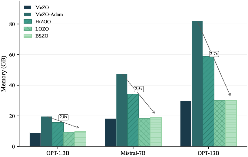
5.4. Memory and Time EfficiencyBSZO keeps memory usage low. As shown in Figure2and Table 4, BSZO’s memory footprint stays close to MeZO across three model scales-ranging from 1.00× to 1.08× of MeZO’s usage. In contrast, HiZOO and MeZO-Adam need 1.73×-1.96× and 2.16×-2.74× more memory because they store additional optimizer states (momentum, Hessian estimates). BSZO avoids this overhead by using only O(k 2 ) extra space for the posterior covariance and adaptive noise estimation.BSZO runs fast.Table 4 also reports per-step time. BSZO and LOZO are the fastest-both under 100ms per step on OPT-1.3B. HiZOO is roughly 2× slower due to Hessian estimation, and MeZO-Adam incurs extra cost from momentum updates.

5.4. Memory and Time EfficiencyBSZO keeps memory usage low. As shown in Figure2and Table 4, BSZO’s memory footprint stays close to MeZO across three model scales-ranging from 1.00× to 1.08× of MeZO’s usage. In contrast, HiZOO and MeZO-Adam need 1.73×-1.96× and 2.16×-2.74× more memory because they store additional optimizer states (momentum, Hessian estimates). BSZO avoids this overhead by using only O(k 2 ) extra space for the posterior covariance and adaptive noise estimation.BSZO runs fast.

5.4. Memory and Time EfficiencyBSZO keeps memory usage low. As shown in Figure2and Table 4, BSZO’s memory footprint stays close to MeZO across three model scales-ranging from 1.00× to 1.08× of MeZO’s usage. In contrast, HiZOO and MeZO-Adam need 1.73×-1.96× and 2.16×-2.74× more memory because they store additional optimizer states (momentum, Hessian estimates). BSZO avoids this overhead by using only O(k 2 ) extra space for the posterior covariance and adaptive noise estimation.

5.4. Memory and Time EfficiencyBSZO keeps memory usage low. As shown in Figure2

5.4. Memory and Time EfficiencyBSZO keeps memory usage low. As shown in Figure

5.4. Memory and Time Efficiency

noise under bf16 precision on OPT-1.3B. As k grows, the gap between w/ and w/o adaptive noise becomes more pronounced: at k = 8, the adaptive variant leads by 8.67% on RTE, indicating that adaptive noise yields substantial gains in low-precision settings. Table 5(d) validates this on

School of Mathematics, Sun Yat-sen University, Guangzhou, China. Correspondence to: Zhihong Huang stswzh@mail.sysu.edu.cn.Preprint. January 19,