Logics-STEM Empowering LLM Reasoning via Failure-Driven Post-Training and Document Knowledge Enhancement
📝 Original Paper Info
- Title: Logics-STEM Empowering LLM Reasoning via Failure-Driven Post-Training and Document Knowledge Enhancement- ArXiv ID: 2601.01562
- Date: 2026-01-04
- Authors: Mingyu Xu, Cheng Fang, Keyue Jiang, Yuqian Zheng, Yanghua Xiao, Baojian Zhou, Qifang Zhao, Suhang Zheng, Xiuwen Zhu, Jiyang Tang, Yongchi Zhao, Yijia Luo, Zhiqi Bai, Yuchi Xu, Wenbo Su, Wei Wang, Bing Zhao, Lin Qu, Xiaoxiao Xu
📝 Abstract
We present Logics-STEM, a state-of-the-art reasoning model fine-tuned on Logics-STEM-SFT-Dataset, a high-quality and diverse dataset at 10M scale that represents one of the largest-scale open-source long chain-of-thought corpora. Logics-STEM targets reasoning tasks in the domains of Science, Technology, Engineering, and Mathematics (STEM), and exhibits exceptional performance on STEM-related benchmarks with an average improvement of 4.68% over the next-best model at 8B scale. We attribute the gains to our data-algorithm co-design engine, where they are jointly optimized to fit a gold-standard distribution behind reasoning. Data-wise, the Logics-STEM-SFT-Dataset is constructed from a meticulously designed data curation engine with 5 stages to ensure the quality, diversity, and scalability, including annotation, deduplication, decontamination, distillation, and stratified sampling. Algorithm-wise, our failure-driven post-training framework leverages targeted knowledge retrieval and data synthesis around model failure regions in the Supervised Fine-tuning (SFT) stage to effectively guide the second-stage SFT or the reinforcement learning (RL) for better fitting the target distribution. The superior empirical performance of Logics-STEM reveals the vast potential of combining large-scale open-source data with carefully designed synthetic data, underscoring the critical role of data-algorithm co-design in enhancing reasoning capabilities through post-training. We make both the Logics-STEM models (8B and 32B) and the Logics-STEM-SFT-Dataset (10M and downsampled 2.2M versions) publicly available to support future research in the open-source community.💡 Summary & Analysis
1. **Data and Algorithm Integration**: Viewing the SFT-RL pipeline as a distribution matching problem allows for better integration of data and algorithms to enhance model performance, akin to combining good ingredients to make great food. 2. **Failure-driven Post-training**: Generating data around failure regions guides models to perform better, similar to how students improve by focusing on their weaknesses. 3. **Data Curation Engine**: Combining public and synthetic datasets significantly improves the reasoning abilities of models, much like mixing different ingredients to create a new dish.📄 Full Paper Content (ArXiv Source)
 />
/>
Introduction
In the past years, large language models (LLMs) like OpenAI’s o1 series , QwQ , and DeepSeek-R1 have demonstrated strong performance on challenging reasoning tasks in the field of mathematics and broader STEM. The reasoning capabilities in these models typically emerge from post-training techniques such as supervised fine-tuning (SFT) and/or reinforcement learning (RL) based on strong foundation models. However, while many models are open-sourced, the underlying post-training pipeline and training data curation remain undisclosed, creating both challenges and opportunities for future work.
More recently, the open-source community has made substantial efforts to develop data-construction recipes and algorithmic strategies for cultivating advanced reasoning capabilities in small-scale models, leading to a series of notable works such as Klear-Reasoner , Ring-Lite , MiMo , OpenThoughts , Llama-Nemotron , and AceReason-Nemotron , among others . However, despite these empirical successes, the community still lacks a unified framework to guide data curation and exploitation through post-training algorithms. It is widely recognized in the LLM community that “data is the new oil”, and the algorithm can only succeed when it effectively captures the desired data distribution. This motivates a central question in training reasoning models:
What does it take to build a Data-algorithm Co-design Engine for
Reasoning Models in terms of Effectiveness, Efficiency, and
Scalability?
In this report, we address this question from both theoretical and engineering perspectives. We first provide a data-centric view of the widely adopted SFT-RL pipeline by framing it as a distribution-matching problem. We hypothesize that the first-stage SFT builds a strong proposal distribution that one draws samples for following usage; and the second stage post-training, no matter SFT or RL, shifts the model towards a gold-standard target distribution behind desirable properties such as reasoning ability.
Building on this formulation, we push the boundaries of reasoning models by: (i) implementing a rigorous data curation pipeline to produce a scalable, broad-coverage, and high-quality long CoT dataset as a foundational proposal distribution; (ii) designing an optimized post-training pipeline that utilizes the curated data effectively and efficiently to improve the model’s reasoning capabilities.
Specifically, we curate reasoning data from publicly available datasets and further augment it with synthetic examples generated from documents parsed by Logics-Parsing . Coupled with a fine-grained, difficulty-aware stratified sampling strategy, extensive experiments show that our curated Logics-STEM-SFT-Dataset already equips LLMs with strong foundational reasoning capabilities. Moreover, we adopt a failure-driven post-training paradigm to further align the model with the gold-standard reasoning distribution. Concretely, after the first-stage SFT, we perform targeted knowledge retrieval and synthesize data around the model’s failure regions to guide a second-stage SFT or RL. This yields two alternative pipelines: SFT–RL and SFT–SFT. We systematically test our method under both SFT-RL and SFT-SFT pipelines and show that our approach substantially improves the model’s reasoning ability.
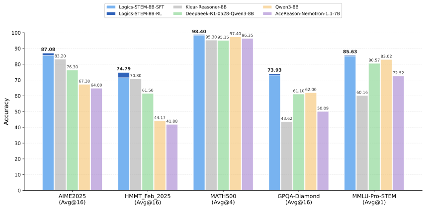
Consequently, we present Logics-STEM, a reasoning model finetuned from Qwen3 that achieves outstanding performance on multiple key reasoning benchmarks. At 8B scale, as shown in 1, Logics-STEM-8B outperforms Klear-Reasoner-8B, DeepSeek-R1-0528-Distill-8B and Qwen3-8B, scoring 90.42% on AIME2024, 87.08% on AIME2025, 74.79% on HMMT2025, 62.5% on BeyondAIME and 73.93% on GPQA-Diamond.
In summary, the contributions of our work are listed as follows.
-
We formulate the SFT-RL pipeline as a distribution matching problem and design a failure-driven post-training framework that leverages targeted knowledge retrieval and data synthesis around model failure regions to effectively and efficiently guide SFT and RL.
-
We design a data curation engine that effectively utilizes publicly available data and augments it with synthetic examples generated from documents. We then produce Logics-STEM-SFT-Dataset, a high-quality and diverse dataset that represents one of the largest‑scale open-source long chain-of-thought corpora at 10M scale.
-
Our reasoning model, Logics-STEM, outperforms other open source models of comparable size on STEM reasoning benchmarks. We release Logics-STEM (8B and 32B) at both the SFT and RL stages, along with the open version of Logics-STEM-SFT-Dataset, to support further research and development within the open-source community.
SFT-RL pipeline as a distribution matching
After pre-training, SFT followed by RL has become a widely adopted recipe for improving LLMs’ reasoning ability . SFT is typically used to familiarize the model with long chain-of-thought (CoT) reasoning traces, while RL further aligns the model with human preferences or sharpens the policy distribution to produce more satisfactory responses with fewer samples . From this perspective, the overall post-training procedure can be viewed as optimizing an expected objective estimated via Monte Carlo sampling. Let the training data consist of pairs $`(x, y)`$, where $`x`$ is the prompt and $`y`$ is the target output (e.g., a long-CoT response ending with a boxed final answer). Denote by $`y^t`$ the $`t`$-th token in $`y`$1. We write the sample-level supervised loss as $`\ell_\theta(x, y)`$ (e.g., the negative log-likelihood, NLL), where $`\theta`$ are the model parameters. The training objective is then,
\begin{equation}
\label{eq:pop_risk}
\text{(Expected Risk)}\quad {\mathcal{L}}^*(\theta)=\mathbb{E}_{(x,y)\sim P^*}\big[\ell_\theta(x,y)\big],
\end{equation}where $`P^*(x,y)`$ denotes the (unknown) ideal target distribution over $`(x,y)`$. However, $`P^*`$ is rarely directly accessible in practice, as it corresponds to a “perfect” or gold-standard distribution for solving reasoning tasks. Instead, one only observes a surrogate dataset $`{\mathcal{D}}`$, which is drawn from some distribution $`P_0(x,y)`$ with $`P_0 \neq P^*`$. This dataset is typically assembled from diverse sources without a unified curation criterion, as we elaborate in 3. Consequently, $`P_0`$ can differ substantially from $`P^*`$, inducing a distribution mismatch between the available training data and the ideal target distribution that would best support reasoning.
The mismatch between target and training distribution.
Practically, a biased optimization is done through minimizing $`\mathbb{E}_{(x,y)\sim P_0}\big[\ell_\theta(x,y)\big]`$ via Monte Carlo estimation, for which one samples mini-batches $`\{x_i, y_i\}_{i=1}^B`$ from $`P_0`$ and approximate the expectation by the empirical mean. To eliminate the bias between target and training, we first look at the issues that cause high expected risk. We consider an importance sampling formula and reformulate [eq:pop_risk] as
\begin{equation}
\label{eq:iw_grad_form}
{\mathcal{L}}^*(\theta)
=\mathbb{E}_{(x,y)\sim P^*}\big[\ell_\theta(x,y)\big]=
\mathbb{E}_{(x,y)\sim P_0}\!\left[
\underbrace{\frac{P^*(x,y)}{P_0(x,y)}}_{\text{Density Ratio}}\underbrace{\,\ell_\theta(x,y)
}_{\text{Sample-wise Loss}}\right],
\end{equation}The high risk of $`{\mathcal{L}}^*`$ is caused by two issues: 1) high density ratio $`\frac{P^*(x,y)}{P_0(x,y)}`$, which means the region is underestimated or rarely seen in training but important in the target distribution; and 2) high sample-wise loss $`\ell_\theta(x,y)`$, which means the model completely fails in these samples.
Remark: From the formula above, we hypothesize that: 1) the first stage SFT is trying to fit the model to a good proposal distribution $`P_0`$, and 2) the second stage RL is trying to explore the region that has a high density ratio and shifts the distribution towards the golden distribution.
We elaborate on the remark a bit. SFT fits the model to $`P_0`$ through a large-scale dataset $`{\mathcal{D}}\sim P_0`$, which provides good proposal distribution with broad coverage and grants the model with general reasoning abilities. However, at this stage, the mismatch between $`P_0`$ and $`P^*`$ would make the optimization biased, thus performing suboptimally on specific tasks. The second stage training is used to implicitly eliminate the bias. For instance, a vanilla policy gradient can be considered as fitting a distribution depending on the advantage function $`A(x,y)`$ ,
\begin{equation}
P^\prime(y \mid x) \propto P_0(y \mid x) e^{\beta A(x,y)},
\end{equation}where $`\beta`$ is the regularization weight. With a proper selection, $`P^\prime`$ can be considered as a good surrogate for the target distribution of $`P^*`$, and the second-stage RL is used to shift the distribution towards $`P^*`$. We provide a detailed discussion in Appendix 9.3.
With this understanding, the second-stage RL can even be replaced by SFT with proper algorithm design, as we will illustrate theoretically in 4 and empirically in 5. As such, we propose two key principles for building a data-algorithm co-design engine for strong reasoning models:
(1) Stage-1 SFT should produce a strong proposal distribution. To this end, we empirically design a data engine that generates high-quality training data, guided by practical experience and engineering insights. 3 details this data engine.
(2) Stage-2 post-training should efficiently shift the model toward the target distribution. In 4, we propose a more effective and efficient way to leverage data to shift the model toward $`P^*`$. Specifically, we introduce a failure-driven resampling for second-stage post-training, enabling target-oriented optimization to enhance reasoning ability.
Reasoning Data Engine
The central goal of the first-stage SFT is to build a diverse, effective, and scalable data engine that learns a proposal distribution $`P_0`$ tailored to reasoning tasks. To this end, we construct long CoT datasets that are rich in reasoning content and generalize well across a wide range of reasoning benchmarks to ensure the $`P_0`$ has a broad support. As shown in 2, our pipeline collects questions from selected sources and produces high-quality reasoning question-response pairs through a series of curation steps.
 style="width:100.0%" />
Data Curation Pipeline
Data Collection.
Previous studies have demonstrated the effectiveness of open-source data. To fully leverage open-source data and ensure diversity, we aggregate questions from a wide range of highly regarded and frequently cited sources on Huggingface2, as listed in Appendix 7.1. For the purpose of preventing potential quality risks, all early synthetic subsets and multi-modal subsets are excluded. Additional, we utilize DEGISNER to incorporate synthetic datasets from books and webpages (DLR-Book and DLR-Web in ) to further scale dataset volume and enhance diversity. All PDF-format documents are parsed into plain text by Logics-Parsing and subsequently processed through the DESIGNER synthesis pipeline.
Annotation.
To unify data curation for the SFT and to further accommodate the subsequent RL with verifiable reward (RLVR) stages, we prompt Qwen3-235B-Instruct-25073 to annotate each sample (including question, meta-data, solution, and answer) across multiple dimensions: (1) whether the question is valid and unambiguous, (2) the discipline and domain associated with the question, (3) the educational level of the question, (4) the answer type, and (5) the verifiable answer (if exists). Samples that do not pass the validity and unambiguity check are subsequently filtered out. Details of annotation are provided in Appendix 7.2.
Deduplication.
To ensure diversity, deduplication is performed at multiple granularities, including both exact and near-duplicate removal. Firstly, we generate an MD5 fingerprint for each question and eliminate redundant samples with identical fingerprints across all sources. Moreover, we apply MinHash-based deduplication using 24 bands with a bandwidth of 10 to identify and eliminate near-duplicate samples. Specifically, within each group of samples sharing the same MinHash bucket, samples with valid questions and verifiable answers are prioritized for retention. Ultimately, approximately two-thirds of the data (about 10 million instances) are retained.
Decontamination.
We perform decontamination against the evaluation benchmarks to eliminate potential contamination in the training data, employing both MinHash-based and N‑gram based methods. Any training sample sharing the same MinHash bucket or an identical 13‑gram with evaluation samples is removed.
Response Distillation.
To balance computational efficiency and response accuracy,
Qwen3-235B-A22B-Thinking-25074 serves as the teacher model to distill
reasoning responses for each question. Generation configurations are
detailed in Appendix 7.3. To suppress systematic bias
during subsequent training, we discard responses that exhibit
degenerative repetition. Concretely, any response with an n-gram
duplication ratio exceeding a predefined threshold is excluded from the
training dataset. Optional further answer verification is conducted
using math-verify library5. In cases where responses do not match
the standard verifiable answers, the teacher model is employed to
regenerate the response once more. The strategy of filtering out
incorrect responses is not adopted, as empirical results indicate that
it leads to degraded performance, consistent with the conclusion of
OpenThoughts .
Weighted Stratified Sampling
Despite the implementation of extensive filtering strategies, the volume
of data generated by our pipeline remains a significant challenge for
model training, thereby necessitating further data sampling. Inspired by
OpenThoughts , we employ a difficulty-based weighted stratified
sampling strategy on STEM-related data to achieve a balance between
reasoning density and data diversity. Specifically, token length of the
response is adopted as a natural and effective proxy for question
difficulty. Our subsequent experiment corroborates the finding of
OpenThoughts that length-based sampling outperforms annotation-based
alternatives.
However, we further observe that purely length-based sampling leads to
degraded model performance on relatively elementary benchmarks (See
Section 5.2.1). To address this
issue, we adopt a stratified sampling strategy for data mixing. In
practice, we compute the quantiles of response token lengths and retain
all samples above the 75th percentile. Samples between the 50th and 75th
percentiles are downsampled by 50%, while those between the 20th and
50th percentiles are downsampled by 10%. This approach ensures a high
reasoning density within the training set while maintaining overall data
diversity.
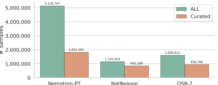
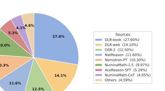
The curated Dataset Statistics
After these fine-grained steps, we obtain Logics-STEM-SFT-Dataset-7.2M before stratified sampling. To the best of our knowledge, it is among the largest open-source long chain-of-thought corpora that is high-quality, diverse, and most importantly, ready for direct use. The overall data flow is shown in 3. We further report the source dataset distribution in 5, and summarize dataset statistics before and after curation for the large-scale open-source sources in 4, highlighting our curation engine’s emphasis on both data quality and diversity. After stratified sampling, we obtain Logics-STEM-SFT-Dataset-2.2M, comprising 1.05M math samples and 1.14M broader-STEM samples distilled from a teacher model to preserve strong reasoning traces.
 style="width:100.0%" />
 />
/>
 />
/>
Failure-Driven Post-training via Knowledge Enhancement
The widely used post-training pipeline consists of two stages: SFT followed by second-stage RL. From our distribution-matching perspective (2), the second stage aims to better approximate the target distribution, and can be implemented via either SFT or RL. Accordingly, in this section we introduce a failure-driven post-training pipeline that is both effective and efficient. Our paradigm is theoretically grounded to better fit the gold-standard distribution for reasoning ability, and is sample-efficient as it correctly leans towards the regions that contribute most to distribution matching.
Algorithmic Design
First-stage Supervised Fine-tuning
Once the data are ready to use, we conduct the first-stage SFT. Considering the token-level decomposition and the supervised loss as the negative log-likelihood (NLL), the training will yield an optimized parameter $`\theta_1`$,
\begin{equation}
\label{eq:stage1-sft}
\theta_1=\arg\min_{\theta}\;\mathbb{E}_{(x,y)\sim P_0}\big[\ell_\theta(x,y)\big],
\quad
\ell_\theta(x,y)=-\sum_{t=1}^{T}\log \pi_\theta\!\left(y^t\mid x,y^{<t}\right).
\end{equation}where $`T`$ denotes the sequence length, $`\pi_\theta(y^t|x, y^{ Although SFT improves LLM performance by fitting the model to a proposal
distribution $`P_0`$, it remains limited on complex reasoning tasks,
especially high-difficulty, cross-domain STEM problems where models
often fail to produce correct answers. This problem reveals that there
is still a distance between $`P_0`$ and $`P^*`$. Thus, to solve the
mismatch between $`P_0`$ and $`P^*`$, we conduct a second-stage
post-training via the following steps: evaluation $`\rightarrow`$
knowledge retrieval $`\rightarrow`$ data synthesis $`\rightarrow`$
continued training. The evaluation helps us identify the regions
$`(x,y)`$ that cause high overall loss (failure regions). Once the
failure region is found, we retrieve from external documents for
knowledge enhancement and synthesize more query-response pairs to
provide more samples and compensate for the density ratio
in [eq:iw_grad_form]. Then, a
second-stage training is done to minimize $`\ell_\theta(x,y)`$ in that
region. After the first-stage SFT and obtaining $`\theta_1`$, the model has
already gained the basic information. To find the regions (i.e.,
query-response pairs) that the model underestimated (high density ratio
between $`P^*`$ and $`P_0`$) or highly biased (high sample-wise loss
$`\ell_\theta(x,y)`$), we evaluate the model on a distribution
constructed from gold-standard evaluation tasks (such as AIME2025 ,
MMLU etc.) denoted as a distribution $`Q`$, and collect failure cases
from this evaluation distribution. We define a failure function
$`w_{\theta_1}(x)\in\mathbb{R}_+`$ to evaluate the value of the current
sample to the model training, which in our implementation is a binary
indicator of verified incorrectness: This induces a failure-driven query distribution which increases the sampling probability of regions where the current
model performs poorly. Under the assumption that $`Q`$ is a proper
surrogate for $`P^*`$, we can show that the new query distribution can
better minimize the expected risk
in [eq:iw_grad_form]. We left the
proof in Appendix 9. Failure resampling alone does not explicitly provide missing knowledge,
as it cannot expand the support of $`P_0`$, and thus can only provide a
better approximation to the existing set. We therefore introduce an
external document corpus $`\mathcal{K}=\{d\}`$ to enhance the
second-stage training, where $`d`$ denotes the external knowledge
document instances. This external document corpus can be retrieved to
further scale up the training dataset. We formalize retrieval as sampling via a kernel. Let $`\varphi(\cdot)`$
be an embedding model and define similarity (via cosine similarity) as
$`s(x,d)=\langle \varphi(x),\varphi(d)\rangle`$, we can define the
conditional sampling distribution over external documents in the
knowledge base as where $`\tau`$ is the temperature to adjust the distribution. In
practice, to enhance the sparsity of retrieval to improve efficiency, we
use a top-$`k`$ truncated variant looks like: Intuitively, $`K_{\tau,k}(d\mid x)`$ specifies how likely a failure case
$`x`$ “activates” a related knowledge document $`d`$, thereby
transferring sampling mass from failure regions to their neighborhoods
in the knowledge space. Given a retrieved document instance $`d`$, we synthesize a new training
example $`(x',y')`$ via powerful LLMs such as DeepSeek R1 . We view
synthesis as another conditional kernel
$`G((x^\prime, y^\prime)\mid d)`$ and apply an acceptance filter
$`a(x^\prime, y^\prime)\in\{0,1\}`$ (e.g., answer-consistency
verification), yielding
$`G_{\mathrm{acc}}(x^\prime, y^\prime\mid d)\propto G(x^\prime, y^\prime\mid d)\,a(x^\prime, y^\prime)`$. Combining failure sampling, retrieval, and synthesis, we obtain the
synthetic data distribution: or equivalently, Thus, the second stage trains on a distribution that mixes
$`P_\text{syn}`$ and $`P_0`$ with percentage $`\lambda`$. Rather than
relying on implicit distribution matching via RL, we argue that SFT can
be used for explicit distribution matching in the second stage, yielding
the following training objective: Equivalently, this is done via sampling datapoints from $`P_0`$ and
$`P_\text{syn}`$ through a percentage of $`\lambda`$. We prove the
following theorem to show that, under mild conditions, the
failure-driven post-training yields better expected loss. Theorem 1 ((Informal) Failure-driven training minimizes the expected
loss.). *Let $`\nabla {\mathcal{L}}^*(\theta)`$ be the ideal target
graident, $`\nabla {\mathcal{L}}_{1}(\theta)`$ be the stage-2 gradient
under the synthetic distribution $`P_{1}`$, and
$`\nabla {\mathcal{L}}_0(\theta)`$ be the gradient under the original
distribution $`P_0`$. Assuming the gradient is normalized such that
$`\|\nabla {\mathcal{L}}_1(\theta)\|=\|\nabla {\mathcal{L}}_0(\theta)\|`$
and $`Q\approx P*`$, the failure-driven construction of $`P_1`$ makes
the gradients better aligned with the target gradient, i.e., Then, for sufficiently small learning rate $`\eta`$, one stage-2
optimization step using $`P_{1}`$ yields no larger target risk than
using $`P_0`$: The vanilla RL objective is Practically, we test our model using GRPO and DAPO , which we defer the
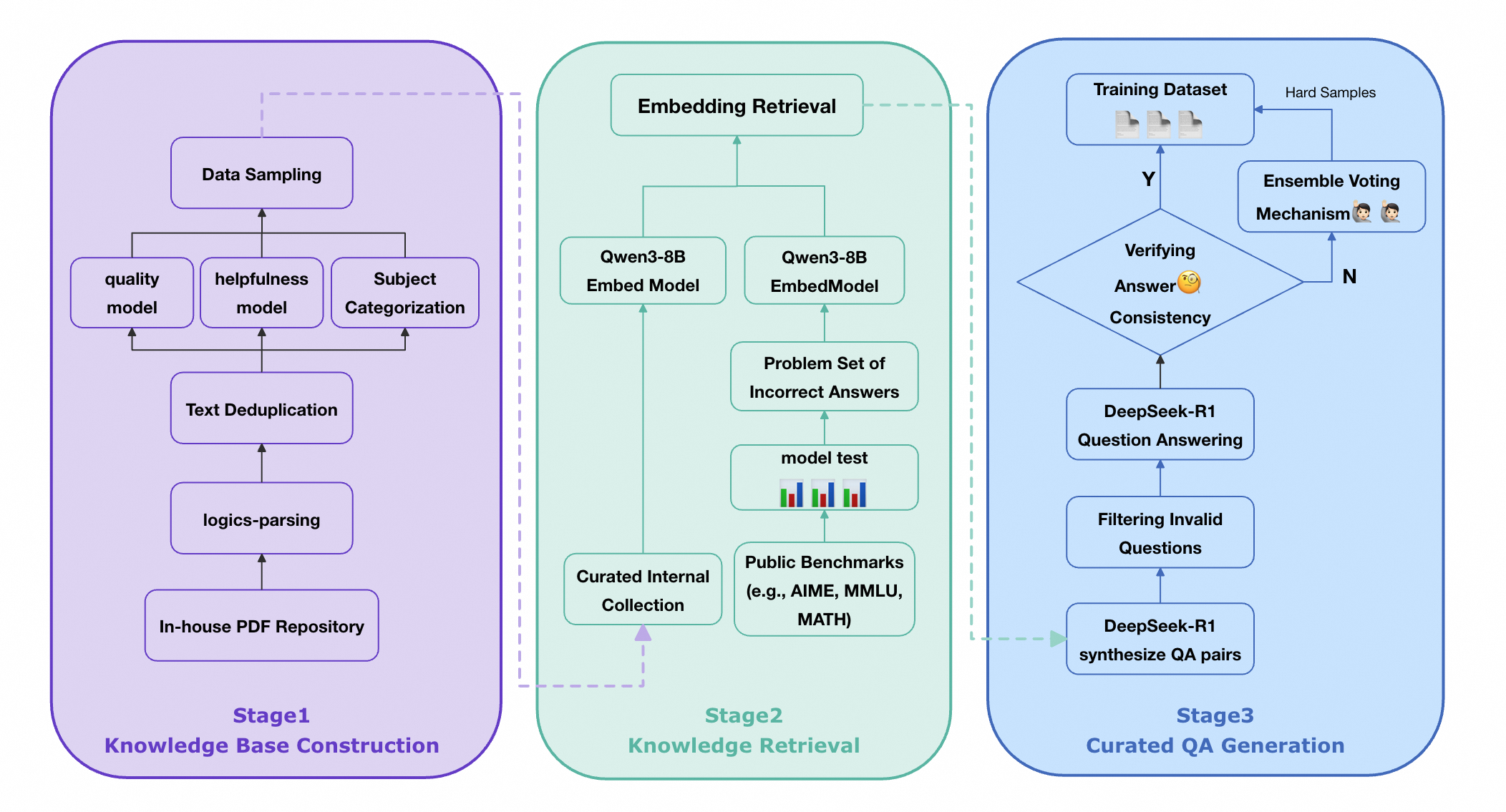
introduction in 4.2.4. We then introduce our engineering implementation. The central tenet of
second-stage training and data usage is to identify the underestimated
region from the failure cases and remediate them using external,
high-fidelity knowledge sources. This is done through three steps: 1)
knowledge base construction, 2) knowledge retrieval engine, and 3)
curated question-answer (QA) pair generation. The overall pipeline is
illustrated
in 7. Notably, data employed in the
second stage is generated automatically without any human annotation. We curated an internal multi-source PDF corpus encompassing academic
papers, technical monographs, authoritative textbooks, and technical
reports. To preserve both structural fidelity and semantic integrity, we
employed LogicsParsing(),a proprietary, high-precision PDF parsing tool,
to convert raw documents into structured HTML format. Subsequently, we
applied a multi-dimensional quality filtering mechanism: A text quality model evaluated linguistic fluency; A usefulness model quantified information richness; A fine-grained subject classification model assigned domain-specific
labels. Only documents exhibiting high fluency, high knowledge density, and
unambiguous domain specificity were retained, culminating in a
high-quality, structurally coherent knowledge base. We first evaluate the SFT model on multiple established STEM benchmarks,
including AIME2025 , MATH500, MMLU that works as the gold-standard
distribution $`Q`$. We then collect questions answered incorrectly as
“knowledge deficiency” samples. These erroneous instances are then
encoded into dense vector representations using the Qwen3-8B-Embed6.
Concurrently, every document in the knowledge base is embedded using the
same model. Leveraging a vector retrieval algorithm, we retrieve the
top-30 semantically most relevant documents for each incorrect question,
ensuring high topical, conceptual, or methodological alignment between
the query and retrieved content. Utilizing the DeepSeek-R1 as the synthesis kernel
$`G((x^\prime, y^\prime)\mid d)`$, we automatically generate two
Query-Response pairs per retrieved document, each requiring deep
reasoning based on the document’s core knowledge points and logical
structure. To guarantee answer accuracy and consistency, a
dual-verification mechanism is implemented to serve as the acceptance
filter: In the first pass, a question and a preliminary answer are generated
jointly; In the second pass, the model is prompted with the question alone to
generate an independent answer; Only samples yielding identical answers across both passes are
retained as high-confidence training instances. For inconsistent cases, we aggregate additional model responses and
applied a majority-voting mechanism to determine a consensus answer;
These samples are incorporated into the training set as “hard examples.”
Furthermore, the length of the Chain-of-Thought (CoT) reasoning trace
generate during the second answer synthesis serves as a proxy indicator
for difficulty, as longer CoT sequences typically signify more complex
reasoning steps and greater challenge. This criterion facilitates the
selection of high-difficulty samples, ensuring the training data not
only possesses high reliability but also effectively stimulates the
model’s potential for advanced reasoning. Through this rigorous
pipeline, we ultimately synthesize a dataset comprising approximately
30K high-quality, high-difficulty, knowledge-aligned QA pairs. This
dataset is subsequently used to train the SFT model, resulting in
substantial improvements in robustness and generalization on complex
reasoning tasks. We test GRPO and DAPO for our framework, which defines the policy
ratio $`r_{i, t}`$ and the renormalized advantage function
$`\hat{A}_{i}`$ as, We adopt the clip-higher strategy alongside batch-level reward
normalization. Specifically, for each $`x\sim P_1(x)`$, we sample
multiple $`\{y_i\}_{i=1}^G`$, and defines the In addition to the answer correctness reward as
in [eq:rl-binary], we add format
compliance and reasoning-length reward to the RL. We use the open-source framework ROLL to compute verified rewards. For
math problems, we use We observe that even when the final answer is incorrect, longer and more
explicit CoT traces often facilitate self-correction and gradual
convergence to the correct solution. Accordingly, we encourage deeper
reasoning by assigning a length-based reward: for incorrect answers, the
reward increases monotonically with the CoT length; for correct answers,
we grant the maximum length reward by default to avoid discouraging
concise yet correct reasoning. We also find that CoT generations can be
redundant. To improve diversity and information density, we incorporate
an $`n`$-gram–based repetition penalty into the reward. Formally, let $`A\in\{0,1\}`$ indicate answer correctness, $`\ell`$ be
the reasoning-trace length, and $`\ell_{\min},\ell_{\max}`$ be length
bounds. We define the normalized length score The final length-aware reward is $`r_{\text{len}} = s(T,A)\cdot \rho,`$
where $`\rho\in(0,1]`$ is a penalty factor computed from the $`n`$-gram
repetition rate of the generated text. With systematic experiments, we show that our framework not only yields
significant gains in reasoning accuracy on STEM benchmarks but also
establishes a novel, reproducible, transferable, and highly efficient
paradigm for data construction in the post-training phase. Models are evaluated on representative reasoning benchmarks spanning
mathematics and broader STEM disciplines. For mathematical reasoning, we
assess performance on AIME2024 , AIME2025, HMMT_Feb_2025, BRUMO2025,
BeyondAIME, and MATH-500. For remaining STEM domains, we adopt
GPQA-Diamond , R-Bench , MMLU-Pro , and CMMLU as benchmarks.
Particularly for MMLU-Pro and CMMLU, we select STEM-related subsets to
specifically evaluate the model’s reasoning capabilities in STEM fields,
as detailed in 7.4. To ensure statistical robustness and mitigate sampling variability, we
conduct $`N`$ independent generations for each test instance using
zero-shot evaluation, adhering to the generation configurations detailed
in 10 by default. For
reasoning-intensive benchmarks with a limited number of test instances,
such as AIME2024, AIME2025, BeyondAIME, HMMT_Feb_2025, and GPQA-Diamond,
we perform $`16`$ generations per case. In contrast, for elementary
benchmarks or those with a larger number of test instances, we use up to
$`4`$ generations per instance. Consequently, we report Pass@1 as the
primary evaluation metric, with additional Pass@K (also referred to as
Best@N) and majority-vote accuracy (Majority@N) as supplementary
metrics. Further details of evaluation settings are described in
8.1. As shown in [tab:3,tab:4], Logics-STEM-8B-RL
significantly outperforms other reasoning models of comparable size from
the community, scoring 90.42% on AIME2024, 87.08% on AIME2025, 74.79% on
HMMT2025, 62.5% on BeyondAIME and 73.93% on GPQA-Diamond. The
consistently strong performance across diverse benchmarks further
evidences the robust domain-generalization capacity of the proposed data
curation strategy, demonstrating the effectiveness of our SFT and RLVR
strategies. Notably, Logics-STEM-8B-SFT achieves reasoning performance comparable to
state-of-the-art open-source reinforcement learning models of similar
scale, such as Klear-Reasoner-8B. This finding demonstrates our ability
to fully leverage high-quality reasoning datasets and further suggests
that, for models of small size, knowledge distillation through SFT can
be as effective as RL-centric post-training. Moreover, as evidenced by the substantial improvements in the
Majority@N on competition-level benchmarks shown in
3, the application of RLVR after supervised
fine-tuning (SFT) significantly enhances model reasoning ability by
further concentrating the probability distribution around correct
answers, even when SFT has already established a strong baseline. As explained in
3.2, further sampling over
the massive outputs of the curation pipeline is essential. Therefore we
conduct a series of ablation experiments to identify the most effective
sampling strategy. Specifically, for each sampling strategy, we
uniformly sample 200K records to construct the training set and
fine-tune the model for one epoch. Length-based sampling has been demonstrated to be an effective sampling
method ; nevertheless, our experiments demonstrate that its exclusive
use degrades the model’s elementary reasoning and generalization
capacities, as reported in
4. the ablation model trained solely
with length-based sampling incurs significant performance drops on
MATH500, MMLU-Pro-Math, and GPQA-Diamond, despite notable gains on
AIME2024, AIME2025, and HMMT2025. Another set of ablation experiments focuses on variants of stratified
sampling. We explore sampling based on the token length of response
generated by the teacher model and the annotated education level of the
question. The results in Table
4 demonstrate that the former serves as
a natural and more effective proxy for question difficulty. We therefore adopt length-based stratified sampling to mitigate
catastrophic forgetting of elementary reasoning capabilities, while
scaling the training set to strengthen advanced reasoning capabilities. To investigate how different types of benchmark-recall document
synthesis affect second-stage training, we construct training data using
two representative benchmarks: (i) Scientific QA (e.g., GPQA), (ii)
Mathematical reasoning (e.g., Math500, AIME2024/2025, and HMMT).
Following a unified data construction pipeline, we generate second-stage
training samples from incorrectly answered questions in these benchmarks
and train models independently. Experimental results demonstrate that
training data synthesized from GPQA errors not only significantly
improves GPQA evaluation performance but also delivers notable
generalization gains across mathematical reasoning benchmarks (e.g.,
AIME, HMMT). In contrast, training data derived solely from mathematical
benchmarks yields limited improvement in overall STEM capabilities. This finding suggests that the complex reasoning patterns inherent in
scientific QA tasks may possess stronger cross-domain transferability,
making them more valuable for enhancing general reasoning abilities. In this section, we examine how different settings and modules influence
the RLVR training process. We present ablation experiments with detailed
results and demonstrate how they inform the design of our final training
recipe. Our experiments cover different loss functions, including Group Relative
Policy Optimization (GRPO) (), Decoupled Clip and Dynamic Sampling
Policy Optimization (DAPO) (). We first conduct ablation studies on Qwen2.5-7B-Instruct using the
DAPO-Math-17K dataset and find that employing the DAPO objective in
conjunction with Reinforce++ as the advantage estimator yields more
stable and consistent improvements. As shown in
6, an early ablation indicates
that the DAPO loss function outperforms the GRPO Loss on our SFT model.
Therefore, the DAPO objective coupled with Reinforce++ as the advantage
estimator is adopted as the final algorithm. Following , we take advantage of dynamic data sampling strategy in our
training pipeline. Specifically, we first drop the responses that are
longer than our default maximum length, it is called overlong length
filter. Also, for the difficulty filter, for each prompt, we will
calculate the average score within the group of all its responses, if it
is lower or greater than our set threshold, the data will not be
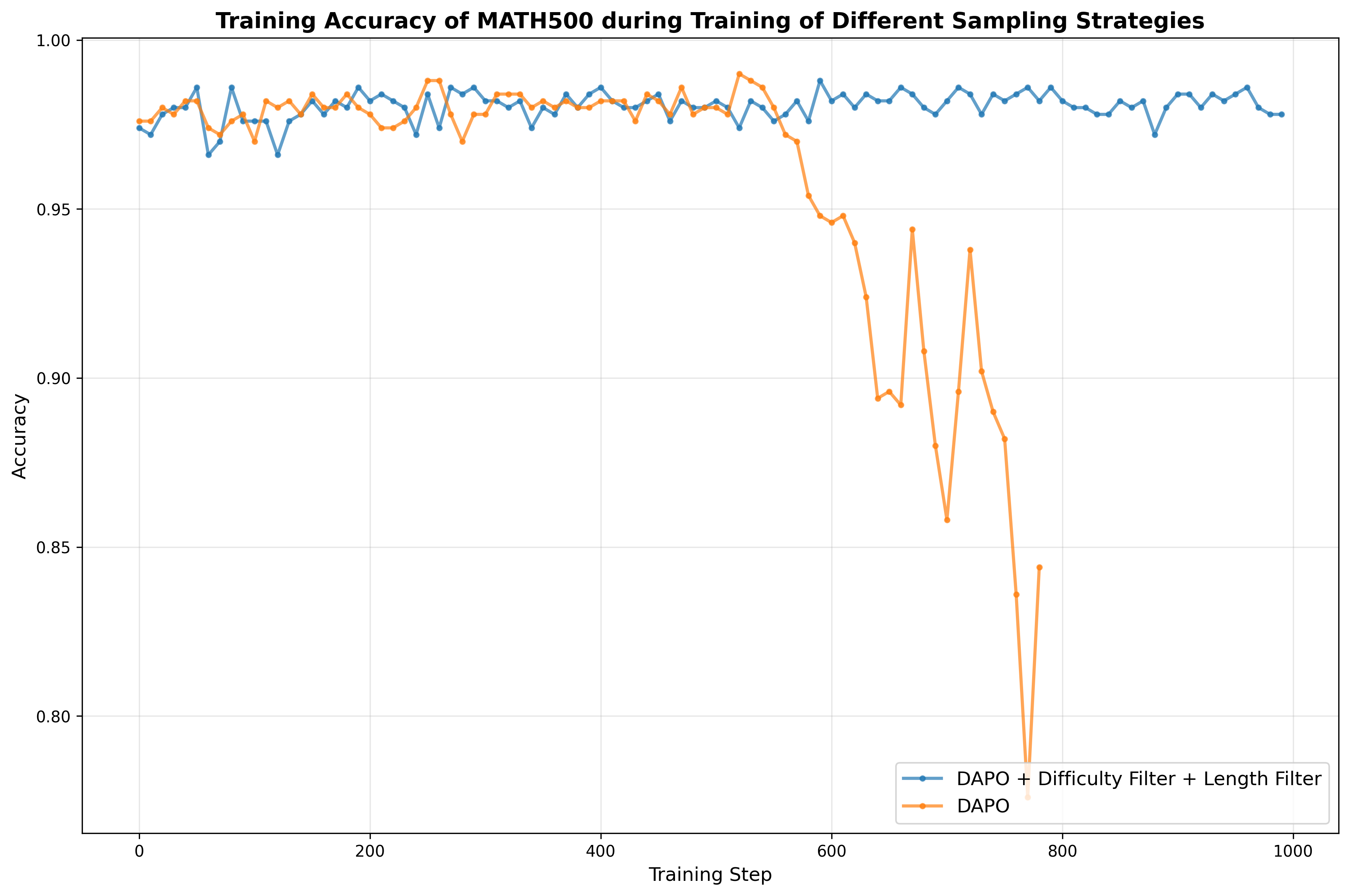
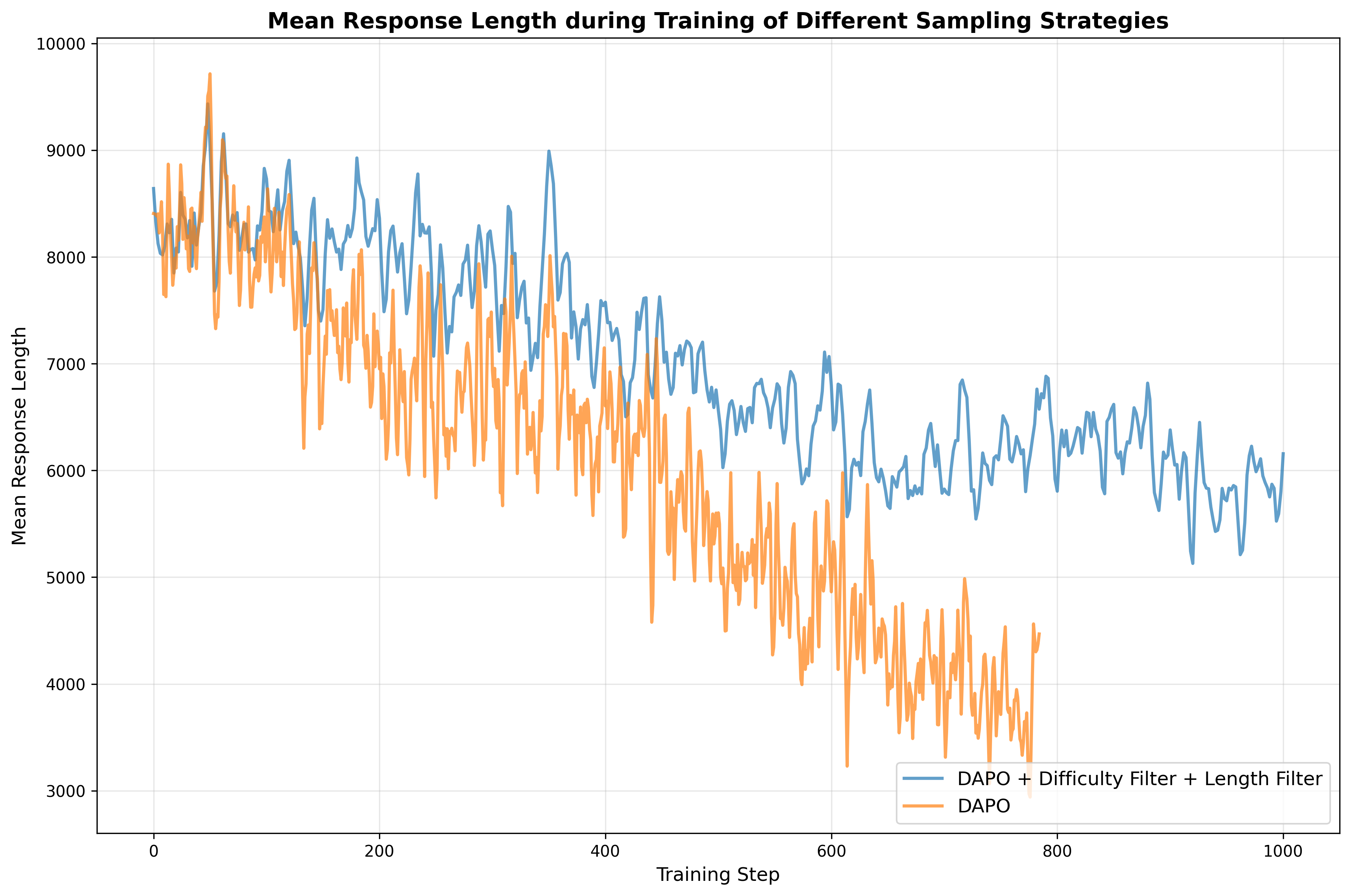
involved in the calculation of loss function. In this experiment, we conduct two groups of trials: one using our
original setting (with both the overlong-length and difficulty filters
enabled), and the other with both filters disabled. We set the lower and
upper thresholds for the average response score to 0.1 and 0.95,
respectively. As we can observe in
8, the group without a filter
tends to collapse in both the training accuracy and response length in
an early stage. Our analysis indicates that response groups with average scores that are
either too high or too low yield near-zero advantage values after
normalization, which in turn results in negligible or zero gradient
updates. Intuitively, such samples are either too “easy” or too “hard”
for the current model and provide little useful signal for learning.
Additionally, without the overlong-length filter, responses exceeding
the maximum allowed length are truncated, making it difficult to extract
the final output and leading to a short response length. Consequently,
both the overlong-length filter and the difficulty filter are essential
to ensure stable and effective training. Experimental results demonstrate that incorporating the reasoning-length
reward and repetition penalty mechanisms yields significant performance
improvements ranging from 2 to 3 percentage points on benchmark
datasets, including AIME2025, HMMT, and CMMLU. Consistent, albeit
modest, gains are also observed across all other evaluated benchmarks. In addition to the superior performance achieved by the model fine-tuned
from Qwen3-8B (as presented in
5.1.3), we also experiment with several
other models as initial models during the supervised fine-tuning (SFT)
stages. All of these experiments further confirm the effectiveness of
our data engine, as shown in 8. Firstly, we fine-tune Qwen3-8B-Base with the identical
Logics-STEM-SFT-2.2M dataset. The resulting model performs on par with,
though marginally weaker than, Logics-STEM-8B-SFT while substantially
surpassing Qwen3-8B. These gains demonstrate that our dataset is
sufficiently diverse and of high quality to support full-scale
supervised fine-tuning (SFT) in the STEM domain. Additionally, we evaluate the scalability of our approach by fine-tuning
Qwen3-32B. Remarkably, the resulting model, Logics-STEM-32B-SFT, still
exhibits substantial improvements in reasoning performance, further
corroborating the high quality of our dataset. In addition to the RLVR experiments, we conduct continual SFT
experiments using failure-driven synthetic data to assess the universal
effectiveness of the data across different post-training paradigms.
Analogous to the RLVR training setup, we conduct experiments on
Logics-8B-SFT, with training hyperparameters detailed in the Appendix.
To mitigate catastrophic forgetting, we experimentally construct
mixtures of 34K failure-driven synthetic data and existing SFT training
data at varying ratios. Notably, under an approximately 1:1 mixture of
failure-driven synthetic data and existing SFT data, the model achieves
improvements comparable to those obtained with the RLVR approach, as
presented in 9 . Due to different evaluation settings in officially reported results that
limit direct comparisons across models, we systematically assess the
effect of inference budget by independently evaluating each model under
varying context settings. As illustrated in [tab:3,tab:4], scaling up inference
budget from 32K context to 64K context leads to significant improvements
on competition-level benchmarks such as AIME2024, AIME2025, and
HMMT2025, whereas improvements on elementary benchmarks remain modest.
The observation is consistent with the intuition that more challenging
problems require deeper deliberation. Moreover, reasoning-oriented
models typically benefit more from the additional inference budget than
the vanilla Qwen3-8B baseline. In an experiment, we apply reinforcement learning on DAPO-Math-17k, a
dataset that exclusively contains numeric verifiable answers. We observe
a marked deterioration in the model’s instruction-following ability,
specifically in its capacity to respond with option letters as
instructed, which leads to significant performance degradation on
GPQA-Diamond, R-Bench, and MMLU-Pro-STEM. This observation explains the
poor performance of Klear-Reasoner-8B on these benchmarks (See
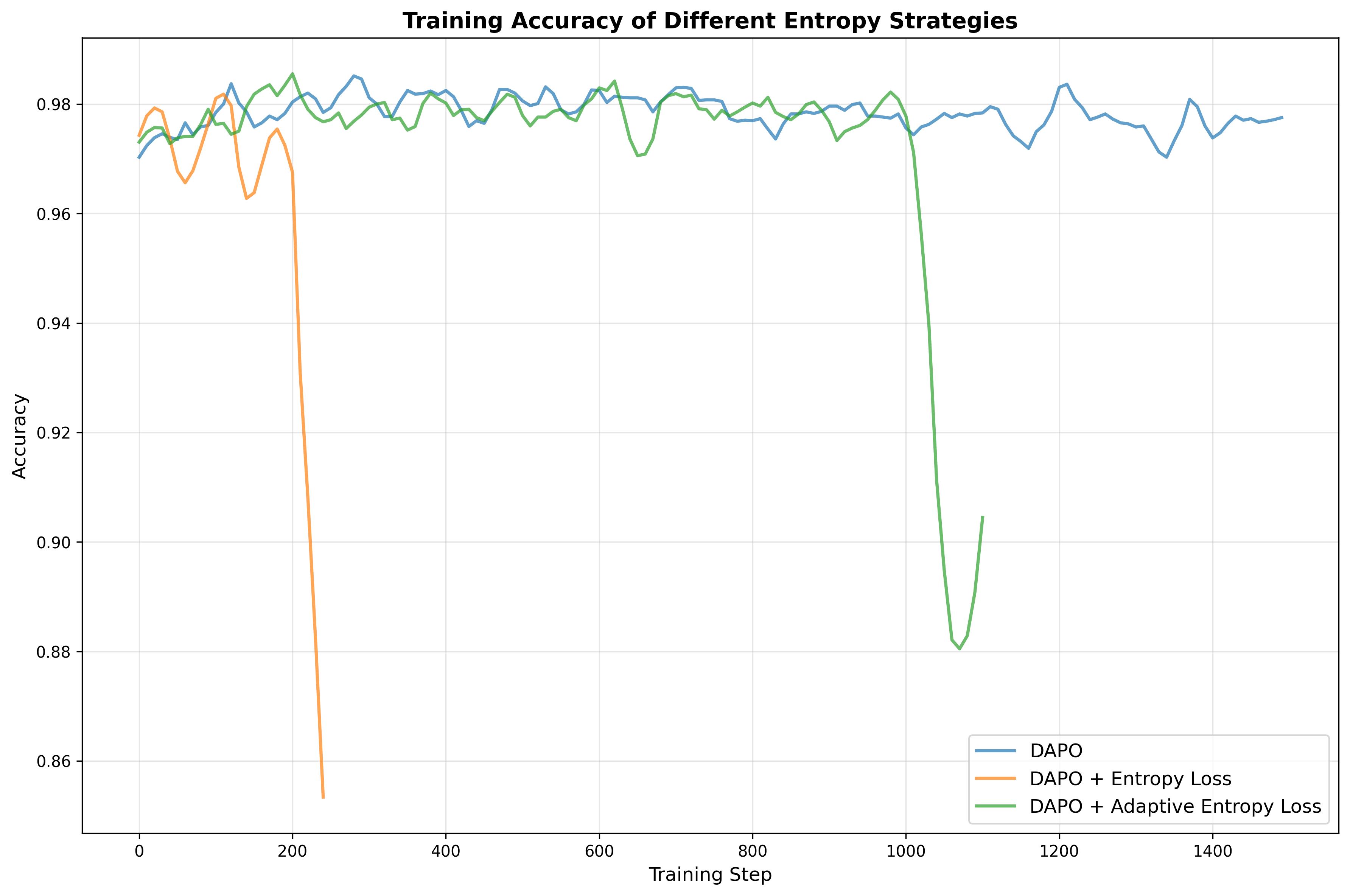
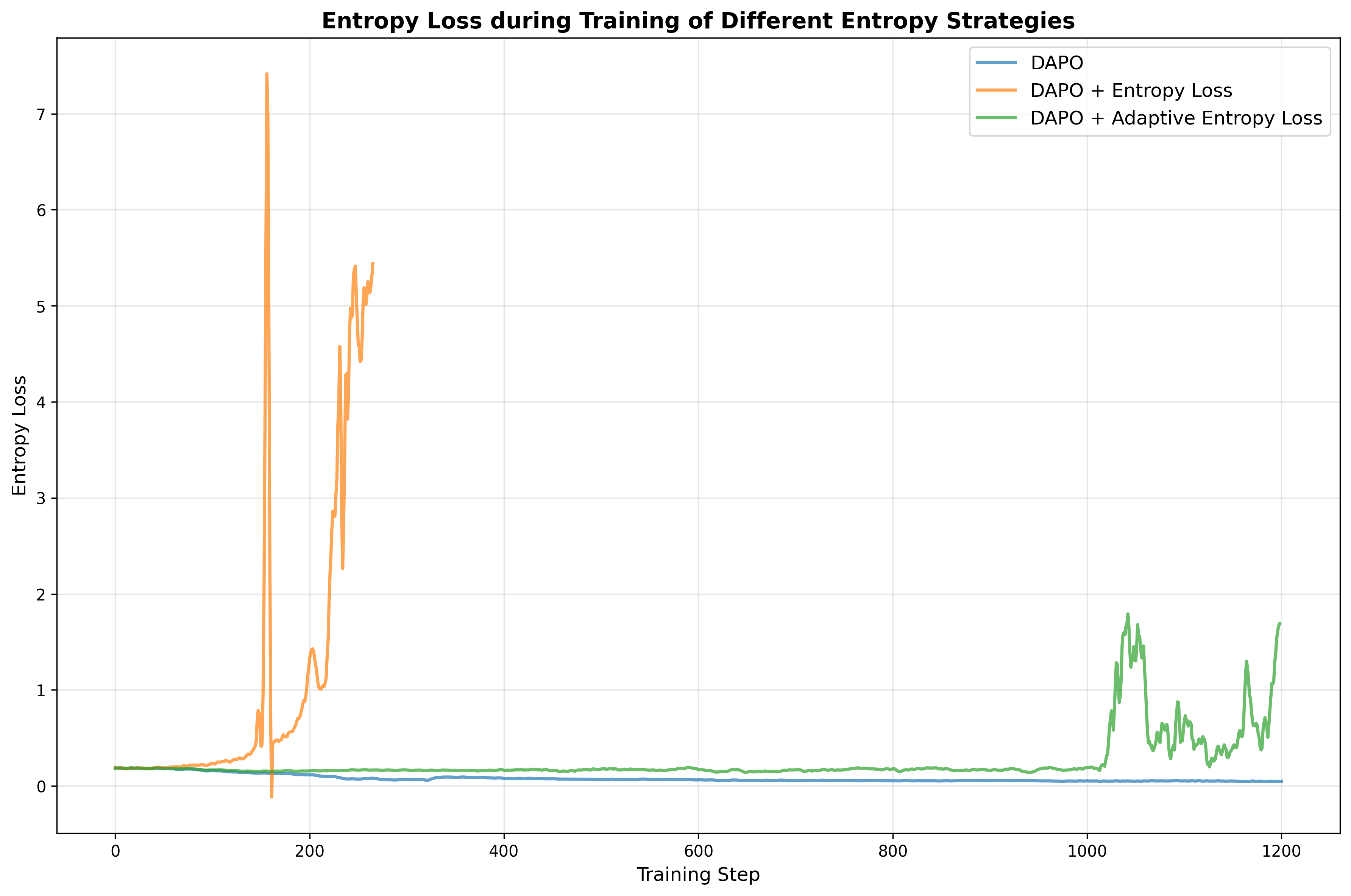
2). In our ablation study, we compare training objectives with and without
an entropy loss term, and we also explore adaptive entropy control
following the approach of , in which we stick to their hyperparameter
setting. Our experiments show that either incorporating a naive entropy
loss or implementing adaptive entropy loss requires careful
hyperparameter tuning and is prone to causing entropy explosion, as
illustrated in
9. Consequently, we exclude this
term from our final training recipe. We further investigate scaling the volume of failure-driven synthetic
data by relaxing the relevance threshold to retrieve more educational
documents associated with each failure case. However, as detailed in
[{appendix: scale
failure-driven}], this actually degrades the model’s performance. We
hypothesize that the additional documents are less strongly related to
the original failures, thereby breaking the expected scaling behavior. This technical report introduces Logics-STEM, a state-of-the-art
reasoning model specifically designed for STEM-related domains. Through
proposed data curation pipeline combined with the difficulty-based
stratified sampling strategy, we effectively select high-quality
reasoning data from both open-access sources and synthetic datasets,
thereby ensuring robust supervised fine-tuning. The further integration
of failure-driven post-training and complementary dynamic sampling leads
to substantial improvements in reasoning performance. For future work,
we plan to further investigate reinforcement learning techniques, scale
the model to larger architectures, and extend its capabilities to a
broader range of tasks, including coding and tool-integrated reasoning. We collect questions from the following highly regarded and frequently
cited datasets: NuminaMath1.5 (), OpenThoughts3 (), Mixture-of-Thoughts
(), AceReason-1.1-SFT (), AceReason-Math (), OpenScienceReasoning-2
7, OpenMathReasoning (), Llama-Nemotron-Post-Training-Dataset (),
DLR-Web (), DLR-Book (), Skywork-OR1-RL-Data (), NaturalReasoning (),
DeepMath-103K (), DAPO-Math-17k (), TheoremQA (), JEEBench (), GPQA-Main
(), GSM8K (), AIME 8, AMC 9, s1-teasers (), s1-probs (),
openaimath (). We structure and organize our reasoning data according to the following
dimensions: Questions are considered invalid and excluded from subsequent curation
if they: (1) lack required images; (2) is incomplete; (3) is
unsolvable. Data are categoried into 6 domains: Math, STEM(excluding Math),
Humanities&SocialScience, Business, Medicine&Biology, Code. Data are categorized by educational level into six tiers: elementary,
junior-secondary, senior-secondary, undergraduate, graduate, and
competition. Answer types are taxonomized as Boolean, multiple-choice, numeric,
vector/matrix, interval, expression, string, proof, textual
explanation, or other. In a narrow sense, verifiable answers include
only multiple-choice and numeric types, while in a broader sense,
verifiable answers further encompass Boolean, vector/matrix, interval,
and expression types. We adopt the recommended configuration parameters provided by Qwen team
for both response distillation and evaluation inference, as detailed in
10. Generation configuration for response generation
As described in Section 3.3, we select STEM-related subsets from
MMLU-Pro and CMMLU to evaluate the model’s reasoning capabilities in
STEM domains. To ensure consistency, we employ a uniform zero-shot evaluation protocol
across all benchmarks, where the model is instructed to enclose its
final answer within $`\backslash`$ Example Two quantum states with energies E1 and E2 have a lifetime
of $`10^-9`$ sec and $`10^-8`$ sec, respectively. We want to clearly
distinguish these two energy levels. Which one of the following options
could be their energy difference so that they can be clearly resolved? For other benchmarks, the following template is adopted: Example Let $`p`$ be the least prime number for which there exists a
positive integer $`n`$ such that $`n^{4}+1`$ is divisible by $`p^{2}`$.
Find the least positive integer $`m`$ such that $`m^{4}+1`$ is divisible
by $`p^{2}`$. We extract the answer from the For each test instance, we calculate three metrics as following: Pass@1 is defined as the average accuracy across $`N`$ rollout
samples. Best@N is assigned a value of 1 if any of the $`N`$ rollout
samples matches the gold answer, and 0 otherwise. Majority@N is assigned a value of 1 if the majority answer among
the $`N`$ rollout samples matches the gold answer, and 0 otherwise. Consequently, we report the evaluation result of each benchmark as the
average of the evaluation metrics computed over all test instances. Hyperparameters we use are listed in [tab:Hyperparam
for SFT,tab: hyperparam for rlvr,tab:Hyperparam for Continual SFT]. Hyperparameters for Supervised Fine-Tuning(SFT)
Hyperparameters for Reinforcement Learning with Verified Rewards(RLVR)
Hyperparameters for Continual Supervised Fine-Tuning(SFT)
We experiment with various entropy-based strategies but failed to
achieve a stable entropy loss or consistent improvements in accuracy
while training, as shown in
9. As described in
5.6, the volume of
failure-driven synthetic data is scaled to 150K. Fine-tuning the model
on a 1:1 mixture of these 150 K synthetic instances and 150 K existing
SFT examples yields the results reported in
14, where we observe
gains only on BeyondAIME and GPQA-Diamond accompanied by performance
drops on all other benchmarks, despite the increased number of training
steps. Consider a model trained by empirical risk minimization (ERM) on the
stage-1 training distribution $`P_0`$: However, our real goal is to minimize the risk under the (unknown)
target distribution $`P^*`$: We can decompose $`P(x,y)=P(x)P(y\mid x)`$, which gives a good
interpretation. In general, $`\hat{\theta}_0 \neq \theta^*`$ because the underlying
measure in the expectation changes from $`P_0`$ to $`P^*`$. This
mismatch manifests in several common failure modes: (1) Covariate/domain shift. The input marginal differs, i.e.,
$`P_0(x)\neq P^*(x)`$, so regions that are frequent under $`P^*`$ may be
rarely sampled under $`P_0`$. When the support overlaps, the target risk
admits an importance-weighted form which highlights that large density ratios $`\frac{P^*(x,y)}{P_0(x,y)}`$
correspond to regions that are under-covered by $`P_0`$ but can dominate
the target risk. (2) Support mismatch. A more severe problem occurs when there exists
a region $`\mathcal{A}`$ such that meaning that the target distribution assigns non-zero mass to inputs
never seen during stage-1 training. In this case, ERM on $`P_0`$ cannot
provide guarantees on $`\mathcal{A}`$. This would cause a extremely
large density ratio. (3) Underweighting high-loss regions. Even if $`P_0`$ and $`P^*`$
share support, uniform sampling under $`P_0`$ may assign very small
probability mass to difficult, high-loss examples. As a result, a large
fraction of gradient updates is spent on “easy” regions, while errors
concentrated in a small but critical subset (often over-represented in
target benchmarks) remain insufficiently optimized. (4) Conditional shift in outputs. Finally, the conditional
distribution can differ, i.e., $`P_0(y\mid x)\neq P^*(y\mid x)`$, which
in LLM post-training often appears as differences in solution style,
chain-of-thought structure, or answer formatting. Such mismatches can
lead the model to learn a behavior prior that is misaligned with the
target tasks. Our second-stage data construction explicitly targets these issues by
inducing a new training distribution $`P_{\mathrm{syn}}`$ from model
failures observed on a target set $`Q`$ (ideally, $`Q\approx P^*`$).
Failure-driven resampling shifts training focus toward regions where the
current model performs poorly under the target distribution, mitigating
covariate shift and the underweighting of high-loss regions. Moreover,
embedding-based retrieval defines a kernel which maps failure queries to relevant external documents. By
synthesizing new training instances conditioned on the retrieved
documents, we effectively expand the support of the training data,
addressing support mismatch by assigning non-zero probability to regions
that were absent in $`P_0`$. Finally, the synthesis prompts and
verification filters allow us to better align output formats and
reasoning traces with target requirements, partially reducing
conditional shift. Theorem 2 (Failure-driven training minimizes the expected loss.).
*Let $`\nabla {\mathcal{L}}^*(\theta)`$ be the ideal target graident,
$`\nabla {\mathcal{L}}_{1}(\theta)`$ be the stage-2 gradient under the
synthetic distribution $`P_{1}`$, and $`\nabla {\mathcal{L}}_0(\theta)`$
be the gradient under the original distribution $`P_0`$. Assuming the
gradient is normalized such that
$`\|\nabla {\mathcal{L}}_1(\theta)\|=\|\nabla {\mathcal{L}}_0(\theta)\|`$
and $`Q\approx P*`$, the failure-driven construction of $`P_1`$ makes
the gradients better aligned with the target gradient, i.e., Then, for sufficiently small learning rate $`\eta`$, one stage-2
optimization step using $`P_{1}`$ yields no larger target risk than
using $`P_0`$: provided that: 1) The evaluation distribution $`Q`$ sufficiently covers
the target distribution and mimics $`P^*`$ around the failure region; 2)
The synthesis kernel $`G(y'|d)`$ correctly mimic $`P^*(y\mid x)`$ and 3)
the retrieval kernel $`K(d\mid x)`$ correctly obtain samples similar to
$`x`$.* We partition the data space based on the performance of the current
model $`\theta`$: Success Region ($`\mathcal{S}`$):
$`\mathcal{S} = \{x \mid w_{\theta}(x) = 0\}`$. The model predicts
correctly and the loss is negligible. Failure Region ($`\mathcal{F}`$):
$`\mathcal{F} = \{x \mid w_{\theta}(x) = 1\}`$. The model fails; loss
is high. Let $`y^*(x)`$ denote the ground truth label (from $`P^*`$) for input
$`x`$. We assume that in the success region $`\mathcal{S}`$, the model
is well-converged. The expected gradient is dominated by zero-mean
noise: Consequently, the target gradient is determined by the failure region.
Let $`\mathbf{v}^*`$ be the average gradient direction required to fix
the failures: Let the synthetic gradient be
$`\mathbf{v}_{\mathrm{syn}} = \mathbb{E}_{P_{\mathrm{syn}}}[\ell_\theta(x,y)]`$,
and assume a similarity factor $`\alpha > 0`$: Then we are able to compare the alignment of the vanilla gradient
$`\nabla {\mathcal{L}}_0`$ and the failure-driven gradient
$`\nabla {\mathcal{L}}_1`$ with the target gradient
$`\nabla {\mathcal{L}}^*`$. The original training distribution $`P_0`$
is dominated by easy samples. Let $`\varepsilon= P_0(\mathcal{F})`$ be
the proportion of failure cases in the original dataset, we have The inner product with the target gradient is: Then, recall $`P_1 = \lambda P_0 + (1-\lambda) P_{\mathrm{syn}}`$. The
synthetic distribution $`P_{\mathrm{syn}}`$ concentrates mass on
$`\mathcal{F}`$ and generates gradients $`\mathbf{v}_{\mathrm{syn}}`$. The inner product with the target gradient is: Substituting
$`\nabla {\mathcal{L}}^* \approx P^*(\mathcal{F})\mathbf{v}^*`$: From Eq. equation [eq:align_g0] and
Eq. equation [eq:align_g1], it is realistic to
assume $`\alpha \ge \varepsilon`$, then which implies that Remark. The inequality holds when
$`\alpha \ge \varepsilon\approx P_0(\mathcal{F})`$, where $`\alpha`$ is
the similarity factor between synthetic gradient and true gradient
(typically high approximating 1), and $`P_0(\mathcal{F})`$ is the error
rate on the training set (typically very low (e.g., $`<0.1`$) as the
model fits the training data). $`\alpha`$ is determined by cetrain
properties of $`Q`$, $`K`$ and $`G`$, which we discussed as, $`Q`$ has to approximate $`P^*`$. When $`Q \approx P^*`$, the
evaluation distribution $`Q`$ effectively covers the target failure
region, i.e., $`Q_{\theta}(\mathcal{F}) \approx 1`$. $`K`$ has to correctly retrieve the relevant documents. So the
retrieved $`z`$ are close to $`x`$ around the failure region. $`G(x,y\mid d)`$ jointly need to be close to $`P^*(x,y)`$ and
$`G(y'|d,x)`$ produces synthetic labels $`y'`$ that provide a
descent direction aligned with the ground truth, i.e.
$`y^\prime (x) \approx y^*(x)`$. If retrieval is irrelevant or
synthesis hallucinates (invalid $`K, G`$), then $`\alpha \le 0`$
in [eq:kernel_validity], and
the method fails. Lemma 4 (Gradient alignment yields larger one-step decrease of the
target risk). *Let
$`{\mathcal{L}}^*(\theta)=\mathbb{E}_{(x,y)\sim P^*}[\ell_\theta(x,y)]`$
be the target risk. Assume $`{\mathcal{L}}^*`$ is $`L`$-smooth, i.e.,
for all $`\theta,\theta'`$, Consider two update directions $`g_0`$ and $`g_1`$ at the same parameter
$`\theta`$, and define the updates If the step size satisfies $`\eta\le 1/L`$ and the two directions have
the same norm $`\|g_0\|=\|g_1\|`$, then In particular, among update directions of the same norm, a larger inner
product with the target gradient (i.e., better alignment) guarantees a
smaller target risk after one step.* Proof. Consider a single gradient-based update where $`g`$ is the update direction. Using a first-order Taylor
approximation of $`L^*`$ around $`\theta`$ yields Eq. equation [eq:taylor_first_order] shows
that, for a fixed step size $`\eta`$, the target risk decreases more in
one step when the inner product $`\langle \nabla L^*(\theta), g\rangle`$
is larger. Assume that $`{\mathcal{L}}^*`$ is $`L`$-smooth (i.e., its gradient is
$`L`$-Lipschitz). Then the descent lemma gives: Therefore, for the same step size $`\eta`$, if
$`\langle \nabla {\mathcal{L}}^*(\theta), g_0\rangle \leqslant\langle \nabla {\mathcal{L}}^*(\theta), g_1\rangle`$
makes the update reduce the target risk more effectively, i.e., For stage-2 SFT we typically take Substituting ends the proof. Our failure-driven post-training framework can be naturally extends to
reinforcement learning with verifiable rewards (RLVR). We first show
that RL (with KL regularization) can be viewed as distribution matching
towards a reward-tilted target distribution, and that failure-driven RL
further improves the match to the gold distribution $`P^*`$ by
correcting the mismatch. Let $`\pi_\theta(y\mid x)`$ denote the current policy and
$`\pi_0(y\mid x)`$ be a reference policy (the stage-1 SFT model), which
serves as a strong proposal distribution with broad support. Consider
the following KL-regularized RL objective : where $`A(x,y)`$ is the advantage of some verifiable reward (e.g.,
correctness/format/length), and $`\beta>0`$ controls the strength of the
KL penalty. For any fixed $`x`$, the maximizer
of [eq:kl_rl_objective] admits a
closed form: [eq:reward_tilted_optimal_policy]
shows that KL-regularized RL performs an exponential tilting of the
proposal $`\pi_0`$ by the advantage, thereby inducing an implicit target
conditional distribution. Moreover, [eq:kl_rl_objective] is
equivalent to a KL-based distribution matching problem: Therefore, a second-stage RL procedure can be interpreted as pushing
$`\pi_\theta(\cdot\mid x)`$ towards $`\pi^*_\beta(\cdot\mid x)`$, i.e.,
matching a target distribution $`P^*(y\mid x)`$. In practice, the overall goal is to reduce the target risk under the
unknown gold distribution $`P^*(x,y)`$. Even if RL improves the
conditional distribution $`P(y\mid x)`$, a mismatch on the prompt
marginal can still lead to suboptimal optimization signal. Concretely,
standard RL typically samples prompts from a surrogate prompt
distribution (e.g., the stage-1 prompt marginal $`P_0(x)`$), while the
true target prompt marginal under $`P^*`$ may emphasize different
regions (especially hard STEM problems). Our failure-driven data construction defines a new prompt distribution As discussed previously, $`P_1(x)`$ better mimic the real distribution
$`P^*(x)`$, thus provides a better estimation to the target
distribution. As a result, RL updates are computed using samples that
are more representative of the hard regions that dominate the target
risk, yielding a better approximation to the ideal distribution-matching
objective. Under $`P_1(x)`$, the KL-regularized RL objective becomes Thus, analogous to [eq:reward_tilted_optimal_policy],
[eq:rl_under_p1] corresponds to
matching the joint distribution where $`P_1(x)`$ is the surrogate prompt distribution and
$`P^\prime(y\mid x)\propto P_0(y\mid x)\exp\big(\beta A(x,y)\big)`$ is
the surrogate Response distribution. Overall $`P^{*}_{\beta,1}(x,y)`$
provides better estimated risk over the gold distribution $`P^*(x,y)`$
when $`P_1(x)`$ is a better surrogate of the target prompt marginal and
$`P^\prime(y\mid x)`$ is a good Response distribution. . The proof
follows almost the same
as 9.2, thus we omit it here.
We use subscripts $`y_i`$ to denote the $`i`$-th training example
and superscripts $`y^t`$ to denote the $`t`$-th token within an
example. ↩︎ https://huggingface.co/Qwen/Qwen3-235B-A22B-Instruct-2507
↩︎ https://huggingface.co/Qwen/Qwen3-235B-A22B-Thinking-2507
↩︎ https://huggingface.co/datasets/nvidia/OpenScienceReasoning-2
↩︎ https://huggingface.co/datasets/di-zhang-fdu/AIME_1983_2024
↩︎The Failure-driven Second-stage Training
Evaluation for failure region identification.
\begin{equation}
\label{eq:binary-failure}
w_{\theta_1}(x)\in\{0,1\}, \quad
w_{\theta_1}(x)=1 \;\;\text{iff the verified final answer of $\pi_{\theta_1}$ on $x$ is incorrect}.
\end{equation}\begin{equation}
\label{eq:failure-biased-q}
Q_{\theta_1}(x)=\frac{Q(x)\,w_{\theta_1}(x)}{\mathbb{E}_{x\sim Q}[w_{\theta_1}(x)]},
\end{equation}Retrieval kernel induced by embeddings.
\begin{equation}
\label{eq:kernel-full}
K_{\tau}(d\mid x)=\frac{\exp\!\big(s(x,d)/\tau\big)}{\sum_{d'\in \mathcal{K}}\exp\!\big(s(x,d')/\tau\big)},
\end{equation}\begin{equation}
\label{eq:kernel-topk}
K_{\tau,k}(d\mid x)\propto \exp\!\big(s(x,d)/\tau\big)\cdot \mathbf{1}\!\left[d\in \mathrm{Top-}k(x)\right].
\end{equation}Data synthesis and the induced synthetic training distribution.
Second Stage Post-training.
\begin{equation}
\label{eq:psyn}
P_{\mathrm{syn}}(x^\prime, y^\prime)
=
\mathbb{E}_{x\sim Q_{\theta_1}}\;
\mathbb{E}_{d\sim K_{\tau,k}(\cdot\mid x)}\!\left[
G_{\mathrm{acc}}(x^\prime, y^\prime\mid d)
\right],
\end{equation}\begin{equation}
\label{eq:psyn-sum}
P_{\mathrm{syn}}(x^\prime, y^\prime)
=
\sum_x Q_{\theta_1}(x)\sum_d K_{\tau,k}(d\mid x)\,G_{\mathrm{acc}}(x^\prime, y^\prime\mid d).
\end{equation}\begin{equation}
{\mathcal{L}}_1(\theta) \triangleq \mathbb{E}_{(x,y)\sim P_1}\big[\ell_\theta(x,y)\big],\quad P_1 = \lambda P_0 + (1-\lambda) P_{\mathrm{syn}}.
\end{equation}\begin{equation}
\langle \nabla {\mathcal{L}}^*(\theta), \nabla{\mathcal{L}}_1(\theta)\rangle
\ge
\langle \nabla {\mathcal{L}}^*(\theta), \nabla {\mathcal{L}}_0(\theta)\rangle,
\end{equation}\begin{equation}
{\mathcal{L}}^*(\theta-\eta \nabla {\mathcal{L}}_1(\theta)) \le {\mathcal{L}}^*(\theta-\eta \nabla {\mathcal{L}}_0(\theta)).
\end{equation}
```*
</div>
</div>
We left the proof and detailed derivation
in <a href="#app:grad_alignment" data-reference-type="ref+label"
data-reference="app:grad_alignment">9.2</a>.
### Extension to Reinforcement learning
Our framework is derived under the purpose of dealing the mismatch
between training and target distribution, thus it can be naturally
extended to design a second stage training under reinforcement learning
via verified reward (RLVR). We do not elaborate the theoretical proof in
the main text, as it follows a similar structure as failure-driven SFT,
but only show the algorithm here. The detailed derivation can be found
in <a href="#apdx: ext_RL" data-reference-type="ref+label"
data-reference="apdx: ext_RL">9.3</a>
#### Stage-2 RLVR.
We first sample the prompts from the marginal distribution $`P_1(x)`$.
Then, for a prompt $`x`$, the model samples an output
$`y\sim \pi_\theta(\cdot\mid x)`$ and receives a verified reward as the
advantage function $`A`$, where
``` math
\begin{equation}
\label{eq:rl-binary}
A(x,y)\in\{0,1\},
\quad
A(x,y)=1 \;\;\text{iff the final answer in $y$ is verified correct}.
\end{equation}\begin{equation}
\label{eq:stage2-rl}
{\mathcal{L}}(\theta) = \mathbb{E}_{x\sim P_{1}(x)}\;
\mathbb{E}_{y\sim \pi_\theta(\cdot\mid x)}\big[A(x,y)\big].
\end{equation}Engineering Implementation
Knowledge Base Construction
Knowledge Retrieval
Data Synthesis
Reinforcement Learning Implementation
\begin{equation}
r_{i, t}(\theta)=\frac{\pi_\theta\left(y_i^t \mid x, y_i^{<t}\right)}{\pi_{\theta_{\text {old }}}\left(y_{i}^t \mid x, y_{i}^{<t}\right)}, \quad \hat{A}_{i}=\frac{A_i-\operatorname{mean}\left(\left\{A_i\right\}_{i=1}^G\right)}{\operatorname{std}\left(\left\{A_i\right\}_{i=1}^G\right)} .
\end{equation}\begin{equation}
\label{eq: DAPO}
R(x,y) =\left[\frac{1}{\Sigma_{i=1}^{G}|y_i|}\sum_{i=1}^{G}\sum_{t=1}^{|y_i|}\min(r_{i, t}(\theta)\hat{A}_{i}, \text{clip}(1+\varepsilon, 1-\varepsilon, r_{i, t}(\theta))\hat{A}_{i})\right]
\end{equation}Answer Correctness.
math-verify to compare model outputs against
ground-truth answers and assign a binary reward as advantage
$`A_i\in\{0,1\}`$. For multiple-choice questions, we extract the option
in $`\texttt{\textbackslash boxed}\{...\}`$ and match it to the ground
truth. Following , we apply dynamic sampling to filter problematic
training instances by (i) dropping over-length responses and (ii)
excluding prompts whose response-group mean scores fall outside a preset
range. Hyperparameters are summarized in
Table 12.Length and Repetition Aware Reward.
s(T,A)=
\begin{cases}
1, & A=1 \ \text{or}\ T\ge T_{\max},\\
0, & A=0 \ \text{and}\ T\le T_{\min},\\
\dfrac{T-T_{\min}}{T_{\max}-T_{\min}}, & \text{otherwise}.
\end{cases}Experiments
General Evaluation
Benchmarks
Evaluation Setting
General Evaluation Results
Model
Benchmark
2-7
AIME2024
AIME2025
BeyondAIME
HMMT2025
BRUMO2025
MATH500
avg@16
avg@16
avg@16
avg@16
avg@16
avg@4
Qwen3-8B
76.0†
67.3†
42.88
44.17
67.92
97.4†
w/ 64K Context ♣
75.62
69.17
43.88
42.29
68.12
96.3
OpenThinker3-7B
69.0†
53.3†
34.69
42.7†
61.88
90.0†
AceReason-1.1-7B
72.6†
64.8†
44.69
41.88
69.79
96.35
R1-0528-Qwen3-8B
77.18
68.75
42.50
49.17
70.62
94.35
w/ 64K Context ♣
86.0†
76.3†
48.69
61.5†
74.17
95.15
Klear-Reasoner-8B-SFT
75.6†
70.1†
32.06
57.6†
68.96
94.8
w/ 64K Context ♣
82.29
81.88
52.31
67.08
81.46
95.25
Klear-Reasoner-8B
83.2†
75.6†
48.81
60.3†
72.71
95.7
w/ 64K Context ♣
90.5†
83.2†
50.25
70.8†
77.08
95.3
Logics-STEM-8B-SFT
80.62
73.33
44.31
57.71
72.92
97.5
w/ 64K Context ♣
90.42
85.62
61.25
71.46
86.67
98.85
Logics-STEM-8B-RL
80.62
74.79
48.31
57.29
75.83
97.8
w/ 64K Context ♣
90.42
87.08
62.5
74.79
86.46
98.4
Model
Benchmark
2-5
GPQA-Diamond
R-Bench
MMLU-Pro-STEM
CMMLU-STEM
avg@16
avg@1
avg@1
avg@1
Qwen3-8B
62.00†
64.03
83.02
85.69
w/ 64K Context ♣
60.23
63.35
82.99
85.92
OpenThinker3-7B
53.70†
54.71
70.15
72.96
AceReason-1.1-7B
50.09
57.08
72.52
72.21
R1-0528-Qwen3-8B
58.30
62.48
79.41
85.02
w/ 64K Context ♣
61.10†
63.21
80.57
85.02
Klear-Reasoner-8B-SFT
62.12
57.04
79.90
81.80
w/ 64K Context ♣
63.64
64.03
81.62
82.62
Klear-Reasoner-8B
44.76
46.36
59.80
63.90
w/ 64K Context ♣
43.62
49.31
60.16
64.12
Logics-STEM-8B-SFT
72.70
72.21
85.20
85.06
w/ 64K Context ♣
73.11
72.12
85.24
86.82
Logics-STEM-8B-RL
74.31
71.57
85.33
87.87
w/ 64K Context ♣
73.93
73.67
85.63
88.31
Model
Benchmark
2-9
AIME2025
HMMT2025
BeyondAIME
GPQA-Diamond
Maj@16
Best@16
Maj@16
Best@16
Maj@16
Best@16
Maj@16
Best@16
Qwen3-8B
76.67
83.33
53.33
66.67
46.00
65.00
64.14
83.33
w/ 64K Context ♣
83.33
83.33
56.67
66.67
50.00
66.00
62.12
84.85
R1-0528-Qwen3-8B
73.33
86.67
53.33
76.67
48.00
68.00
64.65
89.39
w/ 64K Context ♣
76.67
86.67
63.33
73.33
58.00
72.00
65.66
90.91
Klear-Reasoner-8B-SFT
73.33
83.33
63.33
80.00
34.00
59.00
66.67
90.91
w/ 64K Context ♣
86.67
96.67
76.67
86.67
61.00
78.00
68.69
91.41
Klear-Reasoner-8B
80.00
93.33
73.33
86.67
57.00
75.00
46.46
77.78
w/ 64K Context ♣
83.33
96.67
73.33
83.33
59.00
74.00
46.46
79.80
Logics-STEM-8B-SFT
80.00
90.00
60.00
76.67
46.00
68.00
76.26
91.41
w/ 64K Context ♣
90.00
93.33
76.67
93.33
66.00
80.00
75.25
91.41
Logics-STEM-8B-RL
80.00
90.00
63.33
73.33
50.00
67.00
76.26
91.92
w/ 64K Context ♣
93.33
96.67
83.33
93.33
67.00
82.00
77.27
92.42
Ablation Study of Data
Sampling Strategy
Stratified Sampling.
Difficulty-Based Sampling.
Model
Benchmark
2-6
AIME2025
HMMT2025
MATH500
GPQA-D
MMLU-Pro-STEM
avg@16
avg@16
avg@4
avg@16
avg@1
Purely Length-Based Sampling
55.62
36.88
$\underline{95.35}$
46.88
75.81
Stratified Sampling
w/ Length-Based
$\underline{53.12}$
34.38
95.5
49.91
79.15
w/ Annotation-Based
52.29
$\underline{34.58}$
94.2
$\underline{48.42}$
$\underline{77.82}$
Source of failure-driven Synthetic Data
Algorithm
Benchmark
2-7
AIME2024
AIME2025
HMMT2025
GPQA-D
MMLU-Pro-STEM
CMMLU-STEM
Avg@16
Avg@16
Avg@16
Avg@16
Avg@1
Avg@1
baseline
90.21
85.56
68.96
73.20
85.35
86.82
GRPO
sci-syn-data
90.42
87.08
74.79
73.93
85.63
88.31
math-syn-data
89.79
86.04
70.42
72.70
85.10
87.27
Ablation Study of Algorithms
RLVR Algorithm
Algorithm
Benchmark
2-7
AIME2024
AIME2025
HMMT2025
GPQA-D
MMLU-Pro-STEM
CMMLU-STEM
Avg@16
Avg@16
Avg@16
Avg@16
Avg@1
Avg@1
DAPO
90.83
85.62
72.92
73.96
85.23
87.34
GRPO
91.46
83.54
69.58
73.55
85.29
87.34
Dynamic Sampling
Length-based Reward and Repetition Penalty
Algorithm
Benchmark
2-7
AIME2024
AIME2025
HMMT2025
GPQA-D
MMLU-Pro-STEM
CMMLU-STEM
Avg@16
Avg@16
Avg@16
Avg@16
Avg@1
Avg@1
GRPO
w/ len reward
90.42
87.08
74.79
73.93
85.63
88.31
w/o len reward
90.21
85.00
70.83
73.74
84.87
85.84
The Generalizability of Data Engine
Generalizability of Logics-STEM-SFT-Dataset to Larger-scaled Models
Model
Benchmark
2-7
AIME2024
AIME2025
BeyondAIME
HMMT2025
MATH500
GPQA-D
avg@16
avg@16
avg@16
avg@16
avg@4
avg@16
Qwen3-8B-Base-SFT
81.04
72.92
43.62
57.5
96.85
72.79
w/ 64K Context
88.75
83.33
61.38
68.96
98.45
73.17
Logics-STEM-8B-SFT
80.62
73.33
44.31
57.71
97.5
72.70
w/ 64K Context ♣
90.42
85.62
61.25
71.46
98.85
73.11
Qwen3-32B♣
82.08
73.12
50.00
55.00
96.55
68.18
Logics-STEM-32B-SFT♣
92.71
89.38
63.56
77.92
98.30
76.64
Generalizability of Failure-Driven Data
Model
Benchmark
2-7
AIME2024
AIME2025
BeyondAIME
HMMT2025
MATH500
GPQA-D
avg@16
avg@16
avg@16
avg@16
avg@4
avg@16
Logics-STEM-8B-SFT ♣
90.42
85.62
61.25
71.46
98.85
73.11
Logics-STEM-8B-RL ♣
90.42
87.08
62.50
74.79
98.40
73.93
Logics-STEM-8B-Exp1 ♣
88.75
83.12
59.69
71.04
97.00
70.96
Logics-STEM-8B-Exp2 ♣
90.83
84.79
62.06
72.08
97.35
72.19
Logics-STEM-8B-Exp3 ♣
91.88
85.62
62.69
73.33
97.40
73.33
Scale Inference Budget
Unsuccessful Attempts
Numeric-Answer-Only RLVR
Entropy Loss in RLVR
Scale Failure-Driven Synthetic Data
Conclusion
More about Data
Source of Data
Annotation
Generation Configuration
Parameter
Value
Temperature
0.6
Top-K
20
Top-P
0.95
Max Context Length
32768
STEM Benchmarks
MMLU-Pro-STEM is composed of the following categories extracted from
MMLU-Pro: “math,” “health,” “physics,” “biology,” “chemistry,” “computer
science,” and “engineering.”
CMMLU-STEM is composed of the following subsets from MMLU-Pro:
“high_school_mathematics”, “elementary_mathematics”,
“college_mathematics”, “high_school_physics”, “high_school_chemistry”,
“high_school_biology”, “electrical_engineering”, “conceptual_physics”,
and “college_actuarial_science”.More about Evaluation
Setting
Zero-shot Evaluation
boxed{} in response to each
question.
For benchmarks featuring multiple-choice questions, such as
GPQA-Diamond, MMLU-Pro-STEM, CMMLU-STEM, we prompt the model with the
following template:
A. $`10^-4`$ eV
B. $`10^-11`$ eV
C. $`10^-8`$ eV
D. $`10^-9`$ eV
Please put your final option letter within $$`\backslash`$boxed{}$.
Please put your final answer within $$`\backslash`$boxed{}$.Answer Verification
\boxed{} expression of the model’s
response and evaluate its correctness by comparing it with the
ground-truth answer using the math-verify library.Evaluation Metrics
Training Setting
Hyperparamaters
Parameter
Value
Batch Size
128
Learning Rate
4e-5
Learning Rate Scheduler
Cosine
Warmup Steps
1000
Epoch
3
Parameter
Value
Rollout Batch Size
64
Learning Rate
1e-6
Number of Return Sequences in Group
8
Response Length
32768
Low Threshold for Difficulty Mask
0.1
High Threshold for Difficulty Mask
0.95
Parameter
Value
Batch Size
64
Learning Rate
1e-5
Learning Rate Scheduler
Cosine
Epoch
3
Supplementaries for Ablation Studies in RLVR
Adaptive Entropy Control
Scale Failure-Driven Synthetic Data
Model
Benchmark
2-7
AIME2024
AIME2025
BeyondAIME
HMMT2025
MATH500
GPQA-D
avg@16
avg@16
avg@16
avg@16
avg@4
avg@16
Logics-STEM-8B-SFT ♣
90.42
85.62
61.25
71.46
98.85
73.11
Logics-STEM-8B ♣
90.42
87.08
62.50
74.79
98.40
73.93
Logics-STEM-8B-Exp3 ♣
91.88
85.62
62.69
73.33
97.40
73.33
Logics-STEM-8B-Exp4 ♣
89.58
85.62
64.38
71.67
97.75
74.84
Theoretical Results for Failure-Driven Post-training
The Resources of Failure Modes
Minizing the loss on $`P_0`$ may not minimize the target risk on $`P^*`$.
\begin{equation}
\label{eq:erm_p0}
\hat{\theta}_0=\arg\min_{\theta}\ \mathbb{E}_{(x,y)\sim P_0}\big[\ell_\theta (x,y)\big].
\end{equation}\begin{equation}
\label{eq:erm_pstar}
\theta^*=\arg\min_{\theta}\ \mathbb{E}_{(x,y)\sim P^*}\big[\ell_\theta(x,y)\big].
\end{equation}\begin{equation}
\label{eq:iw}
\mathbb{E}_{(x,y)\sim P^*}\big[\ell_\theta(x,y)\big]
=
\mathbb{E}_{(x,y)\sim P_0}\!\left[\frac{P^*(x,y)}{P_0(x,y)}\,\ell_\theta(x,y)\right],
\end{equation}\begin{equation}
\label{eq:support_mismatch}
P^*(\mathcal{A})>0,\qquad P_0(\mathcal{A})=0,
\end{equation}How failure-driven retrieval-synthesis mitigates distribution mismatch.
\begin{equation}
\label{eq:retrieval_kernel_discuss}
K(d\mid x)\propto \exp\!\big(\langle \varphi(x),\varphi(d)\rangle/\tau\big),
\end{equation}Failure-driven Post-training Provides Better Gradient Estimation
\begin{equation}
\label{eq:grad_sim}
\langle \nabla {\mathcal{L}}^*(\theta), \nabla{\mathcal{L}}_1(\theta)\rangle
\ge
\langle \nabla {\mathcal{L}}^*(\theta), \nabla {\mathcal{L}}_0(\theta)\rangle,
\end{equation}\begin{equation}
{\mathcal{L}}^*(\theta-\eta \nabla {\mathcal{L}}_1(\theta)) \le {\mathcal{L}}^*(\theta-\eta \nabla {\mathcal{L}}_0(\theta)).
\end{equation}
```*
</div>
</div>
**Proof**: We first
prove <a href="#eq:grad_sim" data-reference-type="ref+label"
data-reference="eq:grad_sim">[eq:grad_sim]</a> as a lemma:
<div class="examplebox">
<div id="lemma:kernel_conditions" class="lemma">
**Lemma 3** (Conditions for Failure-Driven Gradient Alignment). *The
failure-driven gradient $`\nabla {\mathcal{L}}_1`$ achieves better
alignment with the target gradient $`\nabla {\mathcal{L}}^*`$ than the
vanilla gradient $`\nabla {\mathcal{L}}_0`$, i.e.,
``` math
\begin{equation}
\langle \nabla {\mathcal{L}}^*(\theta), \nabla{\mathcal{L}}_1(\theta)\rangle
\ge
\langle \nabla {\mathcal{L}}^*(\theta), \nabla {\mathcal{L}}_0(\theta)\rangle,
\end{equation}
\begin{equation}
    \mathbb{E}_{x \sim P(\cdot|\mathcal{S})} [\nabla \ell_\theta(x, y^*(x))] \approx \mathbf{0}.
\end{equation}\begin{equation}
\nabla {\mathcal{L}}^*(\theta) \approx P^*(\mathcal{F}) \cdot \underbrace{\mathbb{E}_{x \sim P^*(\cdot|\mathcal{F})} [\nabla \ell_\theta(x, y^*(x))]}_{\triangleq \mathbf{v}^*}.
\end{equation}\begin{equation}
\label{eq:kernel_validity}
\langle \mathbf{v}_{\mathrm{syn}}, \mathbf{v}^* \rangle \ge \alpha \|\mathbf{v}^*\|^2.
\end{equation}\begin{equation}
\nabla {\mathcal{L}}_0(\theta) = (1-\varepsilon)\mathbb{E}_{{\mathcal{S}}}[\ell_\theta] + \varepsilon\mathbb{E}_{\mathcal{F}}[\ell_\theta]\approx \mathbf{0} + \varepsilon\mathbf{v}^*.
\end{equation}\begin{equation}
\label{eq:align_g0}
\langle \nabla {\mathcal{L}}^*, \nabla {\mathcal{L}}_0 \rangle \approx \langle P^*(\mathcal{F})\mathbf{v}^*, \varepsilon\mathbf{v}^* \rangle = \varepsilon P^*(\mathcal{F}) \|\mathbf{v}^*\|^2.
\end{equation}\begin{equation}
\nabla {\mathcal{L}}_1(\theta) = \lambda \nabla{\mathcal{L}}_0(\theta) + (1-\lambda) \mathbf{v}_{\mathrm{syn}}.
\end{equation}\begin{equation}
\langle \nabla {\mathcal{L}}^*, \nabla {\mathcal{L}}_1 \rangle = \lambda \langle \nabla {\mathcal{L}}^*, \nabla{\mathcal{L}}_0 \rangle + (1-\lambda) \langle \nabla {\mathcal{L}}^*, \mathbf{v}_{\mathrm{syn}} \rangle.
\end{equation}\begin{equation}
\label{eq:align_g1}
\langle \nabla {\mathcal{L}}^*, \mathbf{v}_{\mathrm{syn}} \rangle \approx P^*(\mathcal{F}) \langle \mathbf{v}^*, \mathbf{v}_{\mathrm{syn}} \rangle \ge \alpha P^*(\mathcal{F}) \|\mathbf{v}^*\|^2.
\end{equation}\begin{equation}
\alpha P^*(\mathcal{F}) \|\mathbf{v}^*\|^2 \ge \varepsilon P^*(\mathcal{F}) \|\mathbf{v}^*\|^2
\end{equation}\begin{equation}
\langle \nabla {\mathcal{L}}^*(\theta), \nabla{\mathcal{L}}_1(\theta)\rangle
\ge
\langle \nabla {\mathcal{L}}^*(\theta), \nabla {\mathcal{L}}_0(\theta)\rangle,
\end{equation}
\begin{equation}
\|\nabla {\mathcal{L}}^*(\theta)-\nabla {\mathcal{L}}^*(\theta')\|\le L\|\theta-\theta'\|.
\end{equation}\begin{equation}
\theta_i^+ = \theta - \eta g_i,\quad i\in\{0,1\}.
\end{equation}\begin{equation}
\langle \nabla {\mathcal{L}}^*(\theta), g_0\rangle \le\langle \nabla {\mathcal{L}}^*(\theta), g_1\rangle
\Longrightarrow
{\mathcal{L}}^*(\theta_1^+) \leqslant{\mathcal{L}}^*(\theta_0^+).
\end{equation}\begin{equation}
\label{eq:gd_update}
\theta^+ = \theta - \eta g,
\end{equation}\begin{equation}
\label{eq:taylor_first_order}
{\mathcal{L}}^*(\theta^+) \approx {\mathcal{L}}^*(\theta) + \left\langle \nabla {\mathcal{L}}^*(\theta), \theta^+-\theta \right\rangle
= {\mathcal{L}}^*(\theta) - \eta \left\langle \nabla {\mathcal{L}}^*(\theta), g \right\rangle.
\end{equation}\begin{equation}
\label{eq:descent_lemma}
{\mathcal{L}}^*(\theta^+) \le
{\mathcal{L}}^*(\theta)
- \eta \left\langle \nabla {\mathcal{L}}^*(\theta), g \right\rangle
+ \frac{L\eta^2}{2}\|g\|^2.
\end{equation}\begin{equation}
{\mathcal{L}}^*(\theta_1^+) \leqslant{\mathcal{L}}^*(\theta_0^+).
\end{equation}\begin{equation}
\label{eq:g_is_grad_Lsyn}
g_0 = \nabla {\mathcal{L}}_{0}(\theta),\quad g_1 = \nabla {\mathcal{L}}_{1}(\theta).
\end{equation}Extension to RL: Theory
RL with KL regularization induces a reward-tilted target distribution.
\begin{equation}
\max_{\pi(\cdot\mid x)}
\mathbb{E}_{y\sim \pi(\cdot\mid x)}\big[ A(x,y) \big]
-\frac{1}{\beta}\mathrm{KL}\!\left(\pi(\cdot\mid x)\,\|\,\pi_0(\cdot\mid x)\right),
\label{eq:kl_rl_objective}
\end{equation}\begin{equation}
\pi^*_\beta(y\mid x)
=
\frac{\pi_0(y\mid x)\exp\big(\beta A(x,y)\big)}
{\sum_{y'}\pi_0(y'\mid x)\exp\big(\beta A(x,y')\big)}
\propto
\pi_0(y\mid x)\exp\!\big(\beta A(x,y)\big).
\label{eq:reward_tilted_optimal_policy}
\end{equation}\begin{equation}
\pi^*_\beta(\cdot\mid x)
=
\arg\min_{\pi(\cdot\mid x)}
\mathrm{KL}\!\left(\pi(\cdot\mid x)\,\|\,\pi^*_\beta(\cdot\mid x)\right).
\label{eq:kl_matching_form}
\end{equation}Failure-driven RL improves the fit to $`P^*`$ by correcting the prompt marginal.
\begin{equation}
P_1(x) \;=\; \lambda P_0(x) + (1-\lambda)P_{\mathrm{syn}}(x),
\label{eq:p1_prompt_marginal}
\end{equation}\begin{equation}
\max_\theta
\;\;
\mathbb{E}_{x\sim P_1(x),\,y\sim \pi_\theta(\cdot\mid x)}\!\big[ A(x,y) \big]
\;-\;
\frac{1}{\beta}\,\mathbb{E}_{x\sim P_1(x)}\!\left[\mathrm{KL}\!\left(\pi_\theta(\cdot\mid x)\,\|\,\pi_0(\cdot\mid x)\right)\right].
\label{eq:rl_under_p1}
\end{equation}\begin{equation}
P^{*}_{\beta,1}(x,y)
\propto P_1(x)P_0(y\mid x)\exp\big(\beta A(x,y)\big),
\label{eq:joint_target_under_p1}
\end{equation}
📊 논문 시각자료 (Figures)
![]()

![]()
![]()
![]()
A Note of Gratitude
The copyright of this content belongs to the respective researchers. We deeply appreciate their hard work and contribution to the advancement of human civilization.
Related Posts
Start searching
Enter keywords to search articles
No results found
Try using different keywords