Introduction

Multi-objective combinatorial optimization problems (MOCOPs) have been extensively studied in computer science and operations research , and arise in a wide range of real-world applications, including transportation scheduling and scheduling , feature selection , energy planning , and communication network optimization . Rather than seeking a single optimal solution as in single-objective optimization, MOCOPs involve multiple conflicting objectives and therefore aim to identify a set of Pareto-optimal solutions, known as the Pareto set. A good approximation to the Pareto set should achieve both convergence and diversity. Due to the inherent NP-hardness of combinatorial optimization and the presence of multiple objectives, most MOCOPs are difficult to solve in practice.

Although classic methods, including exact and heuristic algorithms , have long achieved competitive performance in obtaining an approximate Pareto set, they typically require domain-specific knowledge or massive iterative search. Instead, deep reinforcement learning (DRL) has emerged as a transformative approach to address MOCOPs. Unlike supervised learning , DRL eliminates the dependence on labeled datasets. Moreover, compared to heuristic and exact algorithms, DRL demonstrates superior efficiency in identifying near-optimal solutions in a reasonable computational time .

However, despite these advantages, the robustness of DRL solvers for MOCOPs remains considerably underexplored. For single-objective combinatorial optimization problems, prior studies already investigated robustness by conducting experiments on instances drawn from non-i.i.d. distributions and proposed mitigation strategies such as modified training procedures and refined model architectures . When training and test distributions diverge, DRL models may exhibit substantial performance drops on out-of-distribution instances in MOCOP scenarios, potentially due to overfitting to spurious, distribution-specific cues, a phenomenon often discussed as shortcut learning in deep neural networks . This motivates our work on enhancing the out-of-distribution generalizability of DRL solvers for MOCOPs.

In this paper, we propose a robustness-oriented framework for this setting. Unlike existing neural approaches that primarily target in-distribution performance, we systematically evaluate how distribution shifts and preference conditioning affect the performance of DRL solvers. In addition, we introduce adversarial instance generation and robust training strategies to improve generalization across diverse instance distributions. Our main contributions are as follows:

• We introduce a Preference-based Adversarial Attack (PAA) method to target DRL models for MOCOPs. PAA undermines DRL models by generating hard instances that degrade solutions of subproblems associated with specific preferences. The generated instances effectively lower the quality of the Pareto fronts in terms of hypervolume.

• We propose a Dynamic Preference-augmented Defense (DPD) method to mitigate the impact of adversarial attacks. By integrating a hardness-aware preference selection strategy into adversarial training, DPD effectively alleviates the overfitting to restricted preference spaces. It enhances the robustness of DRL models, thereby promoting their generalizability across diverse distributions.

• We evaluate our methods on three classical MOCOPs: multi-objective traveling salesman problem (MOTSP), multi-objective capacitated vehicle routing problem (MOCVRP), and multi-objective knapsack problem (MOKP). The PAA method substantially impairs state-of-the-art DRL models, while the DPD method enhances their robustness, resulting in strong out-of-distribution generalizability.

Related Work

MOCOP Solvers

MOCOP solvers are typically classified into exact, heuristic, and learning-based methods. Exact algorithms provide Pareto-optimal solutions, but become computationally intractable for large-scale problems  . Heuristic methods, particularly evolutionary algorithms   , effectively explore the solution space through crossover and mutation operations , generating a finite set of approximate Pareto solutions in acceptable time. However, their reliance on problem-specific, hand-crafted designs limits their applicability .

Learning-based solvers, particularly those based on deep reinforcement learning, have seen growing adoption in MOCOPs, largely due to their high performance and efficiency. Current research on DRL solvers belongs mainly to two paradigms: one-to-one and many-to-one. In the one-to-one paradigm, each subproblem is addressed by an individual neural solver  . In contrast, the many-to-one paradigm streamlines the computational process by using a shared neural solver to handle multiple subproblems, which outperforms the one-to-one paradigm and delivers state-of-the-art neural solvers. Among them, the efficient meta neural heuristic (EMNH)  learns a meta-model that is rapidly adapted to each preference to solve its subproblem. The preference-conditioned multi-objective combinatorial optimization (PMOCO)  uses a hypernetwork to generate decoder parameters tailored to each subproblem. The conditional neural heuristic (CNH)  leverages dual attention, while the weight embedding model with conditional attention (WE-CA)  employs feature-wise affine transformations, to enhance preference–instance interaction within the encoder. Our study demonstrates that the proposed attack and defense framework is sufficiently general to challenge and robustify models from all three categories.

Robustness of DRL Models for COPs

Robustness COPs have been studied from both theoretical and neural perspectives. From the theoretical side, Varma et al. introduced the notion of average sensitivity, measuring the stability of algorithmic outputs under edge deletions in classical COPs such as minimum cut and maximum matching. On the neural side, several studies have investigated hard instance generation and defense methods to improve the robustness of DRL solvers for COPs. For example, Geisler et al.  proposed an efficient and sound perturbation model that adversarially inserts nodes into TSP instances to maximize the deviation between the predicted route and the optimal solution. Zhang et al.  developed hardness-adaptive curriculum learning methods (HAC) to assess the hardness of given instances and then generate hard instances during training based on the relative difficulty of the solver. Lu et al.  introduced a no-worse optimal cost guarantee (i.e., by lowering the cost of a partial problem) and generated adversarial instances through edge modifications in the graph. In contrast to these approaches that focused on generating hard instances, Zhou et al.  focused on defending neural COP solvers, by an ensemble-based collaborative neural framework designed to improve performance simultaneously in both clean and hard instances.

Preliminaries

Problem Statement

The mathematical formulation of an MOCOP is generally given as:

\begin{equation}
\min_{\pi \in \mathcal{X}} F(\pi) = \big(f_1(\pi), f_2(\pi), \dots, f_m(\pi)\big), \tag{1}
\end{equation}

where $`\mathcal{X}`$ represents the set of all feasible solutions, and $`F(\pi)`$ is an $`m`$-dimensional vector of objective values. A solution $`\pi`$ to an MOCOP is considered feasible if and only if it satisfies all the constraints specified in the problem. For example, the MOTSP is defined on a graph $`G`$ with a set of nodes $`V = \{0, 1, 2, \dots, n\}`$. Each solution $`\pi = (\pi_1, \pi_2, \dots, \pi_T)`$ is a tour consisting of a sequence of nodes of length $`T`$, where $`\pi_j \in V`$.

For multi-objective optimization problems, the goal is to find pareto-optimal solutions that simultaneously optimize all objectives. These pareto-optimal solutions aim to balance trade-offs under different preferences for the objectives. In this paper, we use the following the Pareto concepts :

Definition 1 (Pareto Dominance). Let $`u, v \in \mathcal{X}`$. The solution $`u`$ is defined as dominating solution $`v`$ (denoted $`u \prec v`$) if and only if, for every objective $`i`$ where $`i \in \{1, \dots, m\}`$, the objective value $`f_i(u)`$ is less than or equal to $`f_i(v)`$, and there exists at least one objective $`j`$ where $`j \in \{1, \dots, m\}`$, such that $`f_j(u) < f_j(v)`$.

Definition 2 (Pareto Optimality). A solution $`x^* \in \mathcal{X}`$ is Pareto optimal if it is not dominated by any other solution in $`\mathcal{X}`$. Formally, there exists no solution $`x' \in \mathcal{X}`$ such that $`x' \prec x^*`$. The set of all Pareto-optimal solutions is referred to as the Pareto set $`\mathcal{P} = \{x^* \in \mathcal{X} \mid \nexists x' \in \mathcal{X} \text{ such that } x' \prec x^*\}`$. The projections of Pareto set into the objective space constitute Pareto front $`\mathcal{PF} = \{F(x) \mid x \in \mathcal{P}\}`$.

Decomposition

By scalarizing a multi-objective COP into a series of single-objective problems under different preferences, decomposition is an effective strategy for obtaining the Pareto front in DRL models for MOCOPs. Given a preference vector $`\lambda = (\lambda_1, \lambda_2, \dots, \lambda_m) \in \mathbb{R}^m`$ with $`\lambda_i \geq 0`$ and $`\sum_{i=1}^m \lambda_i = 1`$, the weighted sum (WS) and Tchebycheff decomposition (TCH) can be used to transform an MOCOP into scalarized subproblems, which are solved to approximate the Pareto front.

WS Decomposition. WS decomposition minimizes convex combinations of $`m`$ objective functions under preference vectors, as defined below:

\begin{equation}
g_w(\pi|\lambda) = \sum_{i=1}^m \lambda_i f_i(\pi), \quad \text{with } \pi \in \mathcal{X}.
\label{eq:weighted}
\end{equation}

Tchebycheff Decomposition. Tchebycheff decomposition minimizes the maximum weighted distance between the objective values and an ideal point, defined as:

\begin{equation}
g_t(\pi|\lambda, z^*) = \max_{1 \leq i \leq m} \lambda_i |f_i(\pi) - z^*_i|, \quad \text{with } \pi \in \mathcal{X},
\label{eq:Tchebycheff}
\end{equation}

where $`z^* = (z^*_1, z^*_2, \dots, z^*_m)`$ represents the ideal point, with $`z^*_i = \min_{\pi \in \mathcal{X}} f_i(\pi)`$.

The decomposition strategy addresses an MOCOP by reducing it to a series of subproblems under varying preferences. Given an instance $`x`$ and a preference $`\lambda`$, neural MOCOP solvers learn a stochastic policy $`p_\theta`$ to approximate the Pareto solution $`\pi = (\pi_1, \pi_2, \dots, \pi_T)`$, where $`\theta`$ represents the learnable parameters.

Glimpse of Robustness of DRL Solvers

Given the unexplored robustness of DRL models for MOCOPs, we first examined the performance of two representative neural solvers, PMOCO  and CNH , for MOTSP. Both solvers are pretrained on clean 50-node bi-/tri-objective TSP instances (as in the original papers).

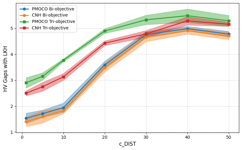
Concretely, we create out-of-distribution test instances using a Gaussian mixture model (GMM) generator for evaluation. We vary $`c_{\text{DIST}} \in \{1, 5, 10, 20, 30, 40, 50\}`$, where $`c_{\text{DIST}}`$ controls the spatial spread of the clusters, which determines the hardness of the instances. WS-LKH (the state-of-the-art solver for MOCOPs) was used as a baseline for comparison. Figure 1 illustrates the HV gaps, representing the difference between the solutions produced by a neural solver and those using WS-LKH:

\begin{equation}
\text{Gap} = \frac{HV_{\text{LKH}} - HV_{\text{DRL}}}{HV_{\text{LKH}}} \times 100.
\end{equation}

Our findings reveal that with increasing $`c_{\text{DIST}}`$ (indicating more difficult test instances), the performance of the neural solvers deteriorates and the gap between their solutions and those provided by WS-LKH widens. These results highlight a significant limitation that neural solvers trained on uniformly distributed instances struggle to maintain robustness as test instances become more diverse and complex.

The Method

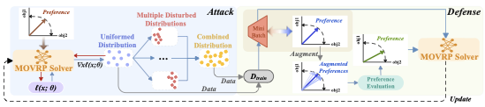
In this section, we introduce a preference-based adversarial attack method to generate hard instances to reflect the robustness of neural solvers. Furthermore, we propose a dynamic preference-augmented defense method to robustify neual solvers. The sketch of the proposed adversarial attack and defense methods is illustrated in Figure 2.

Preference-based Adversarial Attack (PAA)

Typically, neural solvers decompose an MOCOP into a series of subproblems under different preferences, which are solved independently. According to , if a neural solver can solve subproblems ([eq:Tchebycheff]) well with any preference $`\lambda`$, it can generate a good approximation to the whole Pareto front for MOCOP. In this paper, we hypothesize that if a neural model does not effectively approximate the solution of the subproblem under certain values of $`\lambda`$, the resulting approximation of the Pareto front will be inadequate. Following this inspiration, we propose the PAA method to attack neural solvers for MOCOPs. In particular, perturbations are tailored to the original data (i.e., clean instances) in accordance with respective preferences, resulting in hard instances aligned with each specified preference. After identifying hard instances across varying preferences, we gather them into a comprehensive set, which is used to systematically undermine the robustness of a neural solver.

style="width:100.0%" />

Without loss of generality, we evaluate the performance of a neural solver for each subproblem by generating hard instances under the corresponding preference, which maximize a variant of the reinforcement loss, defined as:

\begin{equation}
\ell(x; \theta) = \frac{L(\pi \mid x)}{b(x)} \log p_\theta(\pi \mid x),
\label{eq:loss}
\end{equation}

where $`L(\pi \mid x)`$ represents the loss of the subproblem with a given preference $`\lambda`$ (e.g., using the Tchebycheff decomposition as in Eq. ([eq:Tchebycheff])). $`b(x)`$ is the baseline of $`L(\pi \mid x)`$, which is calculated by $`b(x) = \frac{1}{M} \sum_{j=1}^M L(\pi_j \mid x)`$, where $`M`$ is the number of sampled tours for a batch. $`x`$ denotes the problem-specific input, i.e., node coordinates in TSP. $`p_\theta(\pi \mid x)`$ denotes the probability distribution of the solution $`\pi`$, which is derived from a neural model parameterized by $`\theta`$.

Subsequently, the input $`x`$ corresponding to each preference undergoes the following iterative update:

\begin{equation}
x^{(t+1)} = \Pi_{\mathcal{N}} \left[ x^{(t)} + \alpha \cdot \nabla_{x^{(t)}} \ell(x^{(t)}; \theta^{(t)}) \right],
\label{eq:gradient}
\end{equation}

where $`\theta^{(t)}`$ denotes the best-performing model at iteration $`t`$, $`\mathcal{N}`$ represents the feasible solution space, $`\alpha`$ is the step size, and $`\ell(x^{(t)}; \theta^{(t)})`$ is the reinforcement loss defined in Eq.([eq:loss]). At each iteration $`t`$, the variable $`x^{(t)}`$ is updated by performing gradient ascent on the loss function $`\ell(x; \theta)`$, with the calculated gradients $`\nabla_{x^{(t)}} \ell(x^{(t)}; \theta^{(t)})`$ guiding the update step. The projection operator $`\Pi_{\mathcal{N}}(\cdot)`$ is a min-max normalization, ensuring the updated variables $`x^{(t+1)}`$ remains within a feasible solution space $`\mathcal{N}`$. The iterative process continues until the variable $`x^{(t)}`$ converges towards hard instances for the current given preference.

In summary, the clean instances $`x`$ are initially sampled from a uniform distribution, i.e., the distribution of training instances used by neural solvers. Subsequently, we perturb clean instances using our PAA method under respective preferences $`\lambda`$ to generate diverse hard instances. Ultimately, we gather these instances to construct the set of hard instances $`\mathcal{D}_{\text{hard}}`$, which are used to assess the robustness of the model.

Dynamic Preference-augmented Defense (DPD)

To enhance the robustness of the model, we propose the DPD method, which leverages hard instances $`\mathcal{D}_{\text{hard}}`$ and employs the hardness-aware preference selection method to train the MOCOP solvers.

Perturbative Preference Generation. During the adversarial training phase, for each batch in an epoch, we sample a subset of instances $`\mathcal{D}_{\text{hard}}^\lambda`$ from $`\mathcal{D}_{\text{hard}}`$ along with the corresponding preferences $`\lambda`$. Given a preference vector $`\lambda = (\lambda_1, \lambda_2, \dots, \lambda_m)`$, we generate a set of augmented preferences $`\{\lambda_1', \lambda_2', \dots, \lambda_m'\}`$ to explore the neighborhood of $`\lambda`$. These augmented preferences are dynamically adjusted to emphasize regions where the model exhibits weaker performance. For each preference vector $`\lambda`$, its augmented preferences are computed as:

\begin{equation}
\lambda_i' = \text{Perturb}(\lambda, \delta_i),
\label{eq:7}
\end{equation}

where $`\delta_i \sim \text{Uniform}(-\epsilon, \epsilon)`$ is a small random perturbation. $`i`$ reflects the index of the perturbed preference vector.

Since the perturbation may result in a preference vector that does not satisfy the constraint $`\sum_{k=1}^m \lambda_{i,k}' = 1`$, a normalization step is applied to ensure validity:

\begin{equation}
\lambda_{i,k}' = \frac{\lambda_{i,k}'^{\text{raw}}}{\sum_{j=1}^m \lambda_{i,j}'^{\text{raw}}}, \quad \forall k \in \{1, \dots, m\},
\label{eq:8}
\end{equation}

where $`\lambda_{i,k}'^{\text{raw}}`$ represents the raw preference value after perturbation. By incorporating the normalization step, the generated preferences remain within the valid preference space, ensuring $`\sum_{k=1}^m \lambda_{i,k}' = 1`$ for all augmented preferences.

Hardness-aware Preference Selection. For each augmented preference $`\lambda_i'`$ and hard instance $`x \in D_{\text{hard}}^\lambda`$, the neural solver makes an inference to derive a specific Tchebycheff value (Tch). $`Tch(\lambda_i')`$ quantifies the quality of the solution generated by the model with preference $`\lambda_i'`$, where a smaller $`Tch(\lambda_i')`$ indicates a better quality solution for this preference. $`Tch(\lambda_i')`$ are processed using the following softmax function to compute a relevance score for each preference:

\begin{equation}
P(\lambda_i') = \frac{\exp(-Tch(\lambda_i'))}{\sum_{j=1}^N \exp(-Tch(\lambda_j'))}.
\label{eq:9}
\end{equation}

The preferences $`\lambda_i'`$ that produce the poorest solutions (i.e., the highest $`Tch(\lambda_i')`$) are selected for further optimization. $`N`$ in Eq.([eq:9]) denotes the total number of augmented preference vectors.

The preferences associated with the lowest relevance scores, as identified through $`P(\lambda_i')`$, signify regions that cause lower performance of the solver. These preferences are prioritized for further being involved in the optimization, aiming to improve the robustness and generalizability of the model across diverse preferences. The preference with the smallest $`P(\lambda_i')`$ is selected for further optimization:

\begin{equation}
\lambda_{\text{adv}}' = \arg\min_{i} P(\lambda_i').
\label{eq:10}
\end{equation}

For the selected adversarial preference $`\lambda_{\text{adv}}'`$, the original hard instances $`D_{\text{hard}}^\lambda`$ are reused for training. For each instance $`x \in D_{\text{hard}}^\lambda`$, the loss function is recalibrated as:

\begin{equation}
L(x \mid \lambda_{\text{adv}}') = \max_{1 \leq k \leq m} \lambda_{\text{adv},k}' \cdot |f_k(x) - z_k^*|.
\label{eq:11}
\end{equation}

Training Framework. The proposed adversarial training framework is detailed in Algorithm [alg:paa_dpd]. Each epoch in our training framework comprises two phases: the attack phase and the defense phase. During the attack phase, hard instances tailored to individual preferences are generated and subsequently aggregated for further training. In the defense phase, neural MOCOP solvers are trained on constructed instances. The optimization process employs the REINFORCE algorithm to minimize the loss, which is formulated as follows.

\begin{align}
\nabla \mathcal{J}(\theta) = 
& \mathbb{E}_{\pi \sim p_\theta, s \sim \mathcal{D}_{\text{train}}, \lambda_{\text{adv}} \sim \mathcal{S}_\lambda} \Big[ \nonumber \\
& \quad \big(L(\pi \mid s, \lambda_{\text{adv}}) - L_b(s, \lambda_{\text{adv}})\big) \nonumber \\
& \quad \cdot \nabla \log p_\theta(\pi \mid s, \lambda_{\text{adv}}) \Big],
\label{eq:12}
\end{align}

where $`L_b(s, \lambda_{\text{adv}})`$ is used as a baseline to reduce the variance in the estimation of the gradient. Monte Carlo sampling is used to approximate this expectation, where diverse training samples and randomly selected preferences are used iteratively to optimize the model parameters.

Experiments

In this section, we conduct a comprehensive set of experiments on four MOCOPs: bi-objective TSP (Bi-TSP), tri-objective TSP (Tri-TSP), bi-objective CVRP (Bi-CVRP), and bi-objective KP (Bi-KP) to thoroughly analyze and evaluate the effectiveness of the proposed attack and defense methods. All experiments are executed on a server equipped with an Intel(R) Xeon(R) Silver 4214R CPU @ 2.40GHz and an RTX 3090 GPU.

Baselines and Settings

Instance Distributions for Evaluation. To evaluate the efficacy of the proposed attack approach, we benchmark against four typical instance distributions (clean uniform, log-normal (0,1) with moderate skewness, beta (2,5) with bounded asymmetry, and gamma (2,0.5) with high skewness) as well as ROCO , a learning-based attack method that perturbs graph edges under a no-worse-optimum guarantee and trains an agent with PPO to maximize solver degradation.

Evaluation Setup for Targeted Solvers. We target state-of-the-art neural MOCOP solvers, namely Conditional Neural Heuristic CNH, Meta Neural Heuristic EMNH  , and Preference-Based Neural Heuristic PMOCO. We selected these solvers as they all adopt POMO   as the base model for solving single-objective subproblems. For fair comparisons, we adopt WS (weighted sum) scalarization across all methods. To establish the baseline for the relative optimality gap, we approximate the Pareto front using two non-learnable solvers: WS-LKH for MOTSP and MOCVRP, and weighted-sum dynamic programming (WS-DP) for MOKP.

Metrics. To evaluate the proposed attack and defense methods, the average HV and the average optimality gap are employed. HV provides a comprehensive measure of both the diversity and convergence of solutions, while the gap quantifies the relative difference in HV compared to the first baseline solver.

Implementations. We evaluate PMOCO, CNH, and EMNH using their pre-trained models. Hard instances are generated with 101 and 105 uniformly sampled preferences for the bi- and tri-objective settings, respectively, with 100 clean samples per preference, yielding 10,100 and 10,500 instances. Training uses 10,000 clean samples plus hard instances per epoch, with 3 gradient steps (step size 0.01) over 200 epochs. For testing, 200 Gaussian instances are constructed with $`c_{\text{DIST}} \in [10,20,30,40,50]`$. Other settings (e.g., learning rate, batch size) follow their original papers.

Attack Performance

From Table  [tab:attack1], it can be observed that perturbations based on log-normal, beta, and gamma distributions generally have little effect on reducing the HV value of the solution set. In particular, these perturbations produce higher HV values across various solvers compared to clean instances. This indicates that conventional disturbances struggle to substantially impair the performance of solvers such as WS-LKH and WS-DP. Furthermore, the discrepancies between the solutions generated by these neural solvers and the conventional solver under these distributions are consistently smaller than those observed for clean instances. Hence, despite the heterogeneous nature of these distributions, neural solvers demonstrate robust capabilities to maintain high-quality solutions. In contrast, PAA generates problem distributions that significantly reduce HV values in both classical and neural MOCOP solvers, demonstrating strong and consistent attack effect across all problems and sizes. Notably, it achieves the best attack effect over all cases in Bi-KP.

Furthermore, the HV gaps of different solvers on hard instances generated by PAA and on clean instances are considerably larger. For example, on Bi-CVRP50, the attack against EMNH yields a gap of 4.73%, while on Bi-KP100, the attack against PMOCO reaches 7.09%, significantly exceeding the attack effects by instances generated by the other methods. ROCO-RL shows non-trivial attack capability on a few instances (e.g., a notable 4.41% gap against EMNH on Tri-TSP100), yet PAA consistently surpasses it in most MOCO problems, achieving superior attack performance. This indicates that PAA explicitly exposes the vulnerabilities of diverse neural MOCOP solvers, underscoring its effectiveness in challenging solvers across MOCO problems of different sizes and types.

Defense Performance

To evaluate our defense method, we conducted comparative experiments on EMNH, PMOCO, and CNH trained on uniformly distributed clean instances, alongside their DPD variants trained under the proposed framework. We also included WE-CA , a recent neural solver that employs feature-wise affine transformations at the encoder level, as a state-of-the-art baseline for robustness evaluation. All models (with or without DPD) were evaluated in Gaussian instances. The results are reported in Table [tab:defense]. As shown, DPD-defended solvers (PMOCO-DPD, CNH-DPD, EMNH-DPD, WE-CA-DPD) consistently enhance the performance of neural solvers, achieving overall improvements on all problems. Remarkably, on Bi-TSP20 and Bi-CVRP100, WE-CA-DPD and CNH-DPD achieve the first and second best results, respectively. The improvement is particularly evident on Bi-CVRP100, where WE-CA-DPD improves HV by 2.23% over WS-LKH, the largest gain among all solvers.

In addition, CNH-DPD achieves the best result on Bi-CVRP50. The strong and consistent Bi-CVRP results indicate that models with encoder-level preference-instance interaction mechanism (e.g., CNH, WE-CA) exhibit the most pronounced improvements under DPD. In particular, CNH-DPD and WE-CA-DPD deliver leading performance on Bi-CVRP20/50/100.

Regarding the meta-learning–based solver, EMNH-DPD improves EMNH performance and produces the best result (HV 0.6885, with a runtime of 5.29s) on Tri-TSP20, as well as second-best results on Tri-TSP50 and Tri-TSP100. This demonstrates the versatility of DPD in enhancing solvers across distinct learning paradigms.

In terms of computational efficiency, DPD-defended solvers require considerably less runtime compared to non-learnable solvers. For example, WS-DP requires 17.45 minutes to reach the best HV value on Bi-KP, while CNH-DPD in only 8.49 seconds achieves the same. Overall, these results demonstrate that DPD substantially enhances the robustness of neural solvers, yielding strong generalization to larger problem sizes and distribution shifts.

Ablation Study

Ablation studies were conducted on critical hyperparameters of the proposed attack method, with experiments performed on three-objective 50-node TSP instances.

Impact of Gradient Iteration Counts

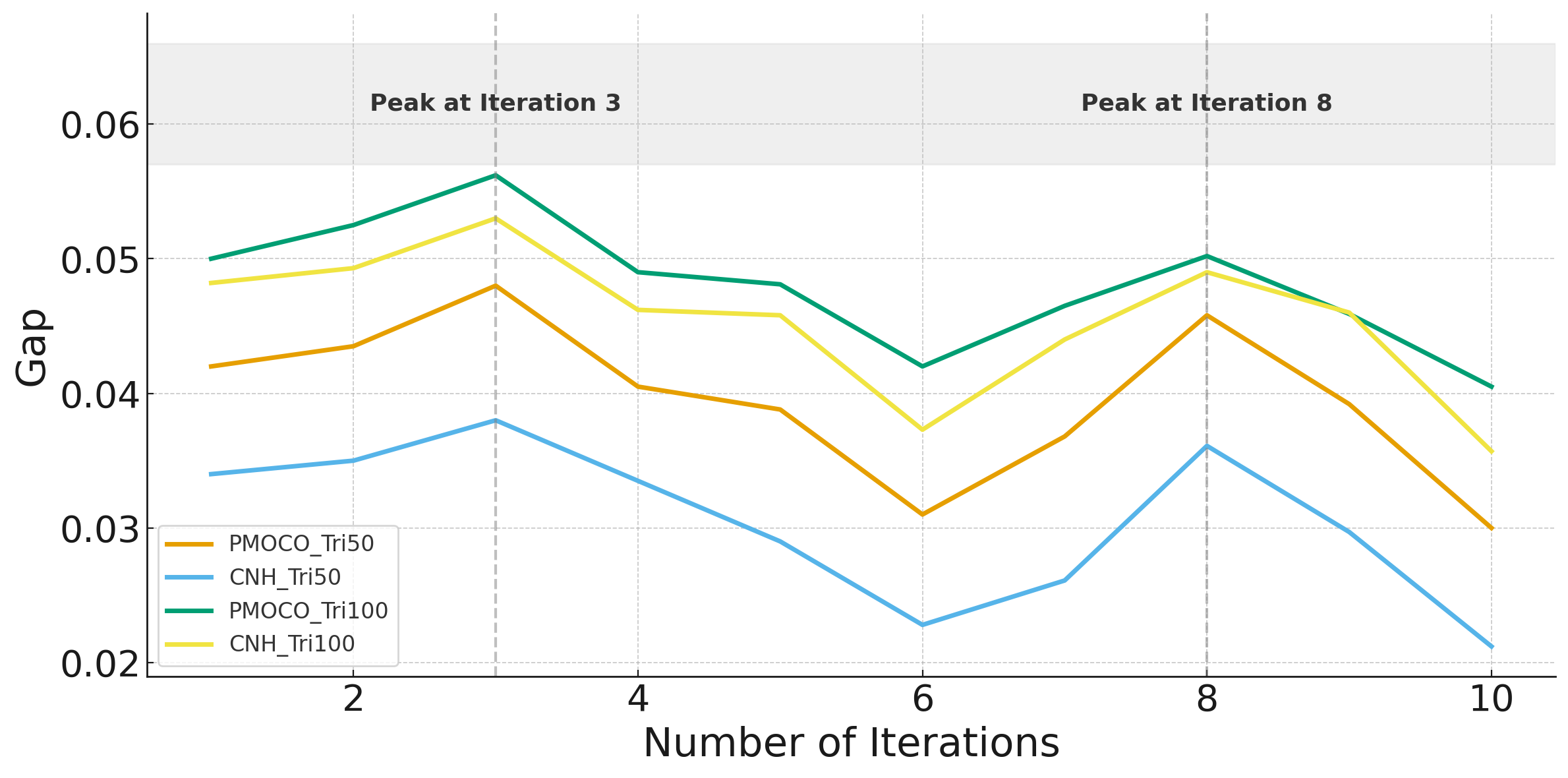
The iteration count $`t`$ in Equation (5) of the main paper is varied from 1 to 10 to evaluate its impact on the HV values and the gap relative to the LKH. As illustrated in Figure  3, the gap peaks at $`t = 3`$ and $`t = 8`$, with the maximum observed at $`t = 3`$. Consequently, $`t = 3`$ is selected in our experiment to balance computational efficiency and performance analysis.

Impact of Gradient Update Parameters

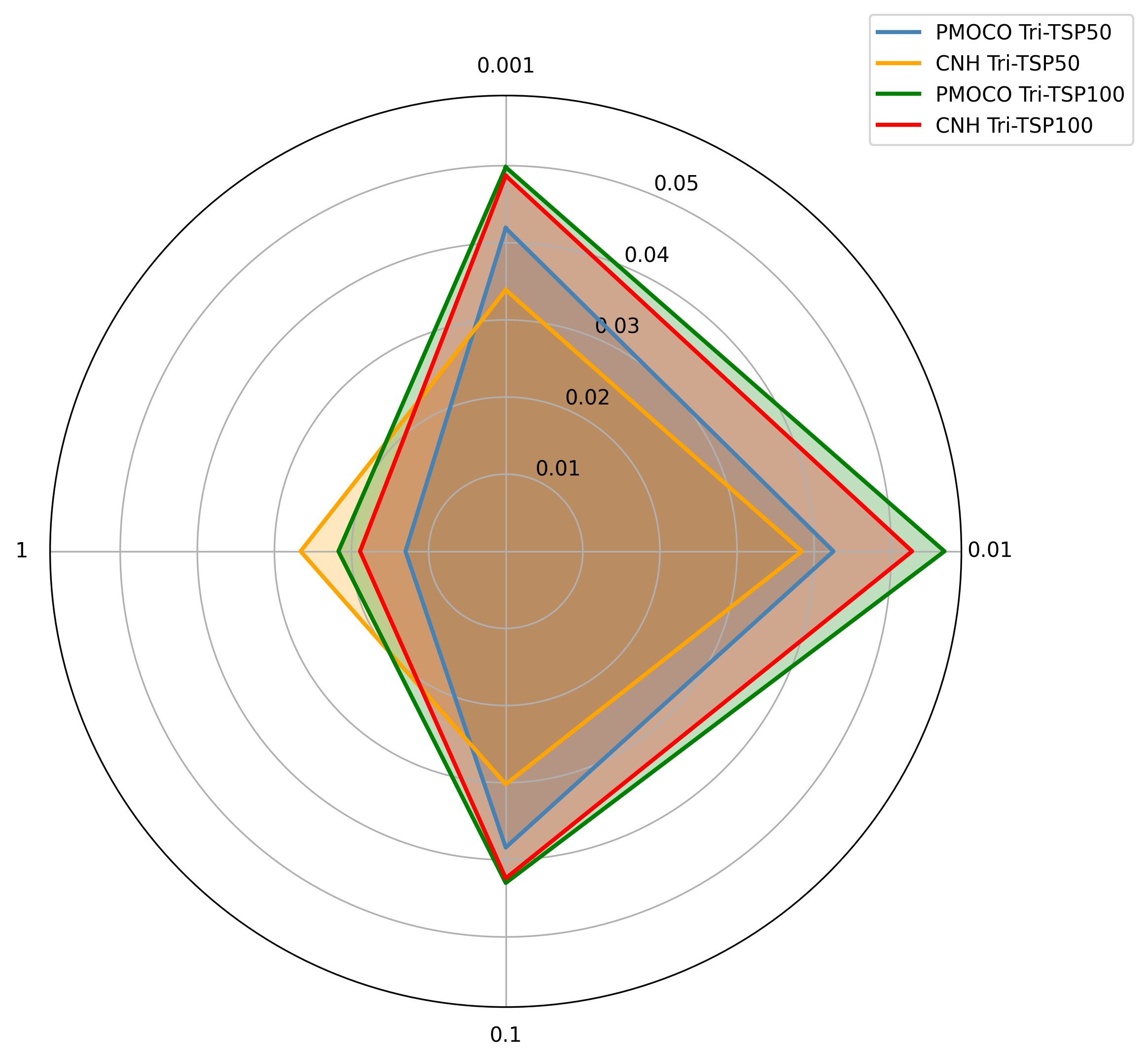
Figure 4 (radar chart) illustrates the relationship between the step size $`\alpha`$ in Equation (5) of the main paper and their HV gaps, showing that the gap reaches its maximum values in $`\alpha = 0.01`$. Therefore, to maximize the effectiveness of the attack, $`\alpha = 0.01`$ is adopted in our experiments.

Robust Training on ROCO-Adversarial Instances

We adopt an offline setting where ROCO is used to pre-generate a pool of adversarial instances, which are then used together with clean data in our DPD framework. For each problem and size, we define a preference grid $`\Lambda`$ (Bi-objective: $`|\Lambda|{=}101`$; Tri-objective: $`|\Lambda|{=}105`$) and draw $`M`$ clean instances per $`\lambda\in\Lambda`$ from the uniform distribution used in the original solvers. Running ROCO on these clean instances under WS scalarization produces an adversarial set for each $`\lambda`$; pooling them yields $`\mathcal{D}_{\text{hard}}^{\text{ROCO}}`$. To ensure fairness, the per-$`\lambda`$ ROCO budget (number of adversarial instances or wall-clock time) is matched across $`\lambda`$ and aligned with the budget used in our PAA experiments.

In each epoch, we build the training set

\begin{equation}
\mathcal{D}_{\text{train}} \;=\; \mathcal{D}_{\text{clean}} \;\cup\; \mathcal{D}_{\text{hard}}^{\text{ROCO}}.
\end{equation}

Mini-batches are sampled by stratified sampling over $`\lambda`$ and data source (clean vs. ROCO), with a default $`1{:}1`$ ratio. We keep the DPD pipeline unchanged: for each mini-batch we generate $`N`$ perturbed preferences $`\{\lambda_i'\}_{i=1}^N`$ in an $`\epsilon`$-neighborhood of the batch preference and renormalize them to the simplex; we compute Tchebycheff values for $`\{\lambda_i'\}`$, form relevance scores via Eq. (8), pick the weakest preference $`\lambda_{\text{adv}}'`$ by Eq. (9), and update the policy by REINFORCE using Eq. (11). All other optimization hyperparameters (optimizer, learning rate, batch size, RL baselines) follow the corresponding original solvers.

We evaluate on Gaussian-mixture test sets (200 instances per setting) with cluster spread $`c_{\text{DIST}}\in\{10,20,30,40,50\}`$ for Bi-TSP and Bi-CVRP at node sizes $`\{20,50,100\}`$. Metrics include mean HV (higher is better), mean relative HV gap (lower is better) computed against WS-LKH (MOTSP/MOCVRP).

As shown in Table [tab:roco-defense], ROCO-trained models (our solvers trained with $`\mathcal{D}_{\text{hard}}^{\text{ROCO}}`$ under DPD) consistently improve HV and reduce optimality gaps over counterparts trained without DPD, while incurring negligible runtime overhead, validating that offline ROCO-adversarial data, when fed through our DPD scheme, yields robust gains under distribution shift.

Benchmark Evaluations

Similarly to previous studies  , we evaluated the performance of our DPD framework on six Bi-TSP100 benchmark instances¹: kroAB100, kroAC100, kroAD100, kroBC100, kroBD100 and kroCD100, which were constructed by combining instances from the kroA100, kroB100, kroC100, and kroD100 instances.

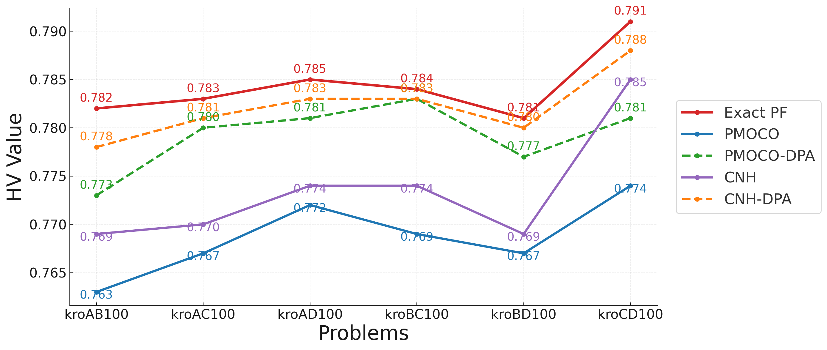
As illustrated in Figure  5, models trained on the hard instances consistently outperform those trained on the clean instances in all the problem instances. The CNH-DPD model achieves the HV values among the learned models, closely approaching the exact PF. In particular, in kroAC100, PMOCO-DPD and CNH-DPD achieve HV values that are 1.4% and 1.7% higher than those of PMOCO and CNH, respectively. In kroBC100 and kroBD100, the HV values for DPD-enhanced models are within 0.1% of the exact PF, demonstrating their competitive performance and robustness. These results underscore the effectiveness of the proposed approach in handling diverse instance distributions and enhancing solver adaptability under adversarial conditions.

Generalization Study

We evaluate the generalization capability of DPD on two types of larger scale test instances ($`n = 150/200`$) including clean instances and mixed Gaussian instances. As illustrated in Table  [table:large], our model demonstrates remarkable robustness across both test scenarios while maintaining strong performance under varying instance distributions.

Conclusions

In this paper, we investigate the robustness and performance of state-of-the-art neural MOCOP solvers under diverse hard and clean instances distributions. We proposed an innovative attack method that effectively generates hard (challenging) problem instances, measuring the vulnerability in solver’s performance by reducing HV values and increasing optimality gaps compared to baseline methods. Furthermore, we also proposed a defense method that leverages adversarial training with hardness-aware preference selection, showing improved robustness across various solvers and tasks. These two methods contribute to solving multi-objective optimization challenges by enhancing the robustness and generalizability of neural solvers, leading to more robust solutions. In the future, we aim to extend our method to address dynamic real-world MOCOP instances, integrating domain-specific constraints, and improving generalizability in online environments.

Acknowledgements

This research did not receive any specific grant from funding agencies in the public, commercial, or not-for-profit sectors.