Flow Equivariant World Models Memory for Partially Observed Dynamic Environments
📝 Original Paper Info
- Title: Flow Equivariant World Models Memory for Partially Observed Dynamic Environments- ArXiv ID: 2601.01075
- Date: 2026-01-03
- Authors: Hansen Jin Lillemark, Benhao Huang, Fangneng Zhan, Yilun Du, Thomas Anderson Keller
📝 Abstract
Embodied systems experience the world as 'a symphony of flows': a combination of many continuous streams of sensory input coupled to self-motion, interwoven with the dynamics of external objects. These streams obey smooth, time-parameterized symmetries, which combine through a precisely structured algebra; yet most neural network world models ignore this structure and instead repeatedly re-learn the same transformations from data. In this work, we introduce 'Flow Equivariant World Models', a framework in which both self-motion and external object motion are unified as one-parameter Lie group 'flows'. We leverage this unification to implement group equivariance with respect to these transformations, thereby providing a stable latent world representation over hundreds of timesteps. On both 2D and 3D partially observed video world modeling benchmarks, we demonstrate that Flow Equivariant World Models significantly outperform comparable state-of-the-art diffusion-based and memory-augmented world modeling architectures -- particularly when there are predictable world dynamics outside the agent's current field of view. We show that flow equivariance is particularly beneficial for long rollouts, generalizing far beyond the training horizon. By structuring world model representations with respect to internal and external motion, flow equivariance charts a scalable route to data efficient, symmetry-guided, embodied intelligence. Project link: https://flowequivariantworldmodels.github.io.💡 Summary & Analysis
#### Key Contributions 1. **Integration of Internal and External Motion**: The paper presents a method to handle both the agent's own motion and the motion of other objects in the environment simultaneously, using 'flow equivariance'. 2. **Enhanced Prediction Performance**: It demonstrates improved long-term dynamic prediction performance in partially observable environments. 3. **Effective Memory Structure**: A memory structure that retains past observations and links them with current observations to predict future states is proposed.Simple Explanation and Metaphors
- Beginner Level: This paper studies how we can accurately model our surroundings and handle the dynamics of moving bodies while also considering our own motion. Think about a hunter coordinating with other animals in a pack hunt.
- Intermediate Level: The paper introduces ‘flow equivariance’ to process time-based symmetries, allowing both internal and external motions to be handled effectively. This leads to better performance compared to existing models.
- Advanced Level: In partially observable environments, the paper proposes handling complex motion dynamics using ‘flow equivariance’, which enables accurate long-term dynamic prediction and improved generalization over longer sequences.
Sci-Tube Style Script
- Beginner Level: Imagine a hunter coordinating with other animals in a pack hunt. This research explores how to accurately understand and predict such complex movements.
- Intermediate Level: Agents need to handle both their own motion and the motion of objects around them. The paper introduces ‘flow equivariance’ to process these motions, leading to better prediction performance.
- Advanced Level: In partially observable environments, predicting dynamic changes over time is challenging. This research proposes a method using ‘flow equivariance’, which allows for accurate long-term predictions.
📄 Full Paper Content (ArXiv Source)
Introduction
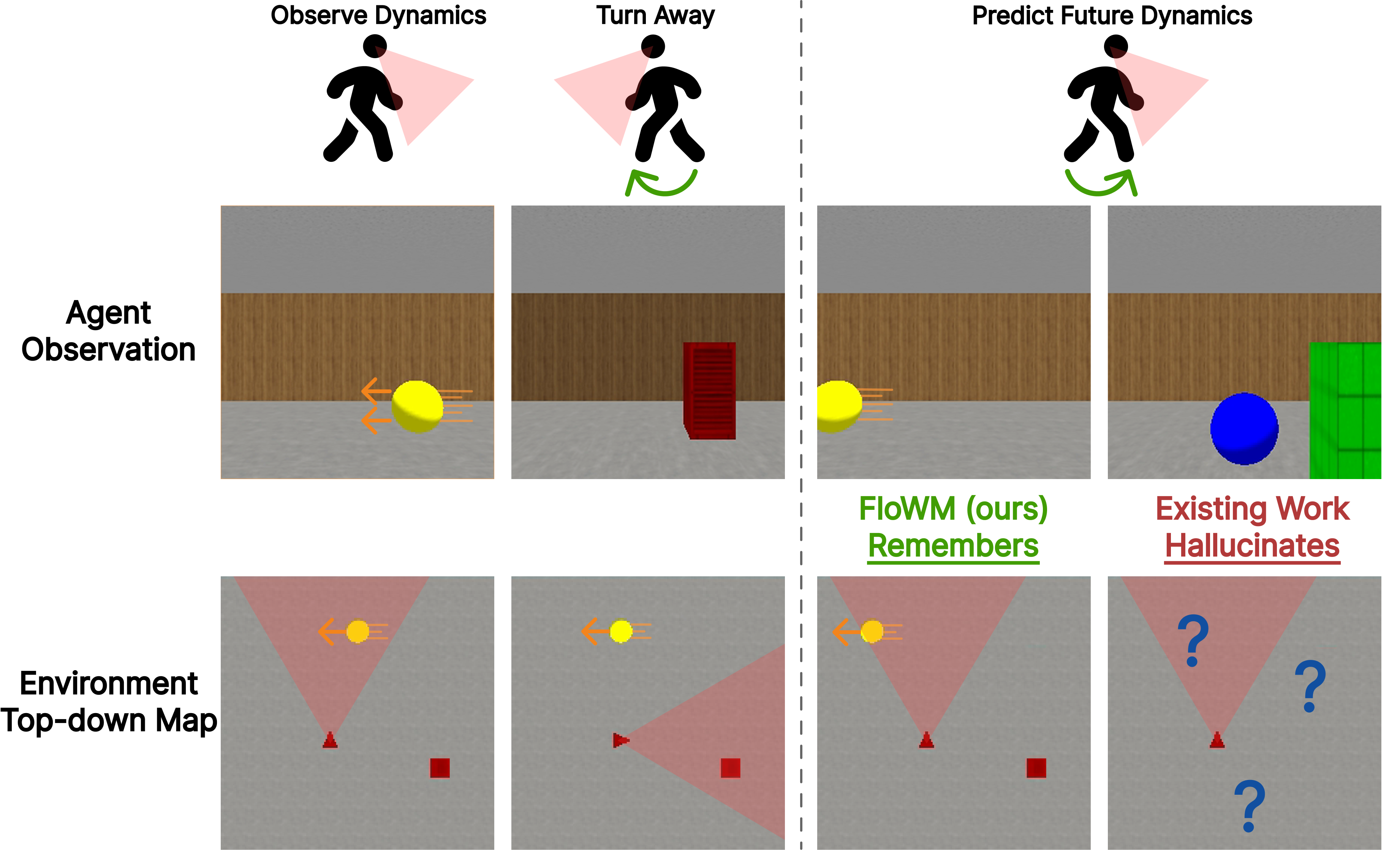
As embodied agents in a dynamic world, our survival critically depends on our ability to accurately model our surrounding environment, our own self-motion through it, and the dynamics of moving bodies within it. A natural example is pack hunting: to coordinate an attack, an agent must accurately estimate the location and velocity of a target while simultaneously predicting the motion of other pack animals. However, these world states are not simply provided to the agent in the form of an omniscient global view; instead, the agent is provided with a restricted first-person field of view that simultaneously shifts and rotates with the agent’s own self-motion. The result is a highly entangled stream of stimulus flows that yields only a fraction of the full environment’s information at any point in time. Despite this, biological agents appear to navigate such partially observed dynamic environments effortlessly, as if they have a latent map of the environment perfectly flowing in unison with the global world state.
In this work, we study the task of partially observed dynamical world modeling (visualized in Fig. 1), combined with the inherent self-motion of embodied agents, and investigate if we might be able to account for both external and internal sources of visual variation in a geometrically structured manner. Specifically, we find that both internal and external motion can be understood as mathematical ‘flows’, enabling both sources of variation to be handled exactly as time-parameterized symmetries through the framework of ‘flow equivariance’ . We demonstrate that we can construct Flow Equivariant World Models that handle self-generated motion in a precisely structured manner, while simultaneously capturing the motion of external objects, even if they are moving outside the agent’s field of view. We show that this yields substantially improved video world modeling performance and generalization to significantly longer sequences than those seen during training, highlighting the benefits of precise spatial and dynamical structure in world models.
Background
To build world models with structured representations of environment dynamics, we rely on recent work in both world modeling and equivariance, which we briefly overview here. More thorough information on related work is available in Section 5 and Appendix 10.
World Modeling.
A world model can be described at a high level as a system affording the ability to predict not only the future state of an environment given initial conditions, but also how that state may evolve differently when acted upon by an agent . Recent work on world models has focused on representing and predicting the future world state as video, primarily using large-scale latent diffusion transformer models. While these models achieve impressive perceptual quality and scale well with growing data and compute, we argue here that their current form inherently lacks the ability to predict long-horizon dynamics in partially observable environments, thus fundamentally limiting their ability to be used for real-world downstream tasks.
Partial observability is defined as a setting when the agent’s observation does not contain the full information of the world’s state. This problem is particularly relevant to world modeling: to accurately make predictions of the future, the model must retrieve all relevant information from previous observations, no matter how long ago it was observed, and bring it to the future prediction. Moving beyond fixed length video generation, recent autoregressive methods such as History-Guided Diffusion Forcing allow extending the transformer self-attention window over many past observation frames to retain self consistency . But inevitably, as the number of observation frames grows, information must be discarded through sliding-window attention or some other approximation. This problem is exacerbated by the cost of spatiotemporal attention over a highly redundant signal such as video. Once the past observation has left the context window (true partial observability with respect to the self attention window), it has been lost; turning around will reveal an entirely new hallucinated scene. Furthermore, relying on information from stale observation frames can be detrimental to modeling the natural dynamics of the evolving world around us.
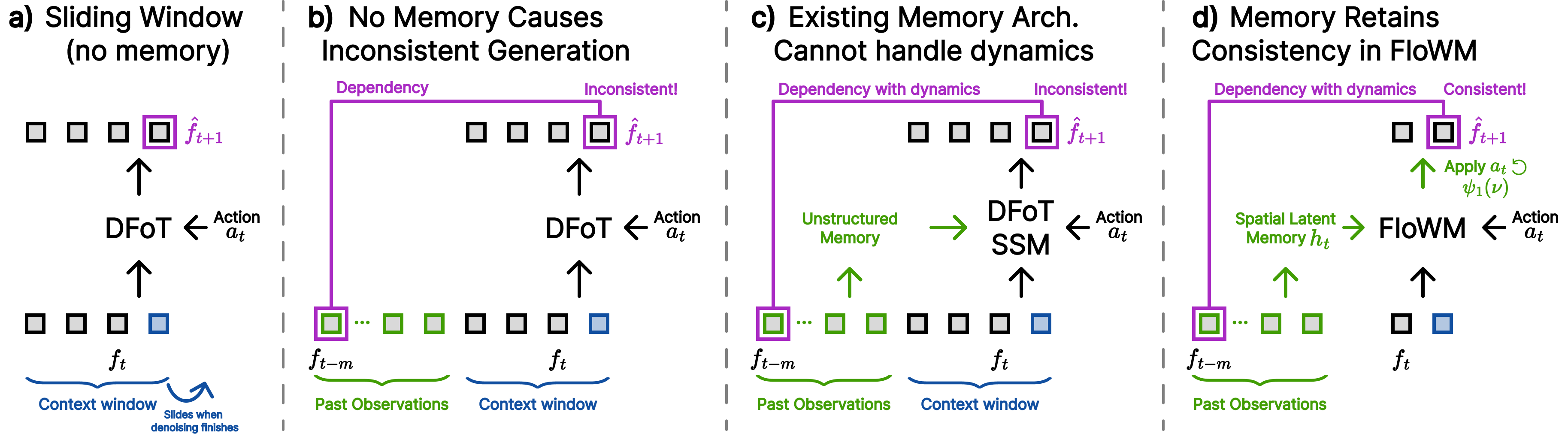
Recent work has explored augmenting video diffusion models with different forms of latent memory that persist across time; however, the focus has primarily been on consistency in static 3D scenes, without a unified framework for modeling partially observed dynamics. In contrast, we argue that a natural way to build world models is with a recurrent flow equivariant memory at the core, evolving and shifting to represent both the dynamics of the world and the actions of the agent seamlessly. Such a memory enables prediction of future states in a precise motion-symmetric manner while maintaining important information for extended observation windows. A visual comparison between modern sliding-window autoregressive transformers, existing memory solutions, and our model (FloWM) is available in Figure 2.
Equivariance.
A neural network $`\phi`$ is said to be equivariant if its output, $`\phi(f)`$, changes in a structured, predictable manner when the input $`f`$ is transformed by an element $`g`$ of the group $`G`$, i.e. $`\phi(g \cdot f) = g\cdot \phi(f) \ \ \forall g \in G`$. One way to construct equivariant neural networks is through structured weight sharing . This structure reduces the number of parameters that need to be learned in an artificial neural network while simultaneously improving performance by incorporating known symmetries from the data distribution. For example, in the setting of molecular dynamics simulation, introducing equivariance with respect to 3-dimensional translations, rotations, and reflections (the group $`E(3)`$, a known symmetry of the laws of physics) increases data efficiency by up to three orders of magnitude .
Flow Equivariant World Models
In this section, we begin with a review of Flow Equivariance, followed by an introduction of a generalized form of the recurrence relation capable of supporting complex tasks. Then, we present instantiations of our general framework for 2D and 3D partially observed dynamic world modeling.
Generalized Flow Equivariance
Flow Equivariance.
Recently, introduced the concept of flow equivariance, extending existing ‘static’ group equivariance to time-parameterized sequence transformations (‘flows’), such as 2d visual motion. These flows are generated by vector fields $`\nu`$, and written as $`\psi_t(\nu) \in G`$. The flow $`\psi_t(\nu)`$ maps from some initial group element $`g_0`$ to a new element $`g_t`$ (i.e. $`\psi_t(\nu) \cdot g_0 = g_t`$), and we can therefore informally think of $`\psi_t(\nu)`$ as a time-parameterized group element when $`g_0`$ is fixed. For example, if we think of $`\nu`$ as a particular velocity, then $`\psi_t(\nu)`$ corresponds to the spatial displacement resulting from integrating $`\nu`$ for $`t`$ time. Formally, a flow $`\psi_t(\nu): \mathbb{R} \times \mathfrak{g} \rightarrow G`$ is a subgroup of a Lie group $`G`$, generated by a corresponding Lie algebra element $`\nu \in \mathfrak{g}`$, and parameterized by a single value $`t \in \mathbb{R}`$ often interpreted as time. A sequence-to-sequence model $`\Phi`$, mapping from $`(f_0,\dots,f_T)\mapsto(y_0,\dots,y_T)`$ is then said to be flow equivariant if, when the input sequence undergoes a flow, the output sequence also transforms according to the action of a flow, i.e.
\begin{equation}
\Phi\left(\{\psi_i(\nu) \cdot f_i\}_{i=0}^T\right)_t = \psi_t(\nu) \cdot \Phi\left(\{f_i\}_{i=0}^T\right)_t \  \forall t,   \label{eqn:flow_eq_orig}
\end{equation}where the action of the flow on a signal $`f_t`$ over the group $`G`$ is defined as the left action: $`\psi_t(\nu) \cdot f_t(g) := f_t(\psi_t(\nu)^{-1} \cdot g)`$. In the case of partial observability, we can modify Equation [eqn:flow_eq_orig] to describe flow transformations acting on a global world state, rather than directly on observations, since objects can move while unobserved and flow equivariant world models should still represent this action faithfully. Formally, we can express this by adding an additional observation function $`\mathcal{O}(w_i)`$ which maps from the global world state ($`w_i`$) to the agent’s current view $`(f_i)`$, and redefining flow equivariance with respect to this world state:
\begin{equation}
\Phi\left(\{\mathcal{O}\left(\psi_i(\nu) \cdot w_i\right)\}_{i=0}^T\right)_t = \psi_t(\nu) \cdot \Phi\left(\{\mathcal{O}\left(w_i\right)\}_{i=0}^T\right)_t \  \forall t,   \label{eqn:flow_eq_po}
\end{equation}In practice, this is mainly a formality, but means output of the sequence model $`\Phi`$ is now defined to be equivariant with respect to the full world state, implying that it is structured to represent more than just the current observation but instead a faithful ‘memory map’ of the dynamic environment.
To achieve flow equivariance, demonstrated that it is sufficient to perform computation in the co-moving reference frame of the input. In other words, for a simple Recurrent Neural Network (RNN), the hidden state must flow in unison with the input, i.e.
\begin{equation}
     h_{t+\Delta t} = \sigma\left(\psi_{\Delta t}(\nu) \cdot h_t + f_t\right).
\end{equation}To achieve equivariance with respect to a set of multiple flows ($`\nu \in V`$), Flow Equivariant RNNs possess multiple hidden state ‘velocity channels’, each flowing according to their own vector fields $`\nu`$ (denoted as $`h_t(\nu)`$), illustrated as stacked rows in Fig. [fig:2d_model_figure](a). Because of the fact that the elements of the Lie algebra combine in a structured manner, it is then possible to show that when the input sequence is acted on by a flow $`\psi(\hat{\nu})`$, the hidden state outputs also flow, and these ‘velocity channels’ permute according to the difference between their velocity and the input velocity ($`\nu - \hat{\nu}`$):
\begin{equation}
 \label{eqn:defn_flow_action}
     h_t[\psi(\hat{\nu}) \cdot f] (\nu) =  \psi_{t-1}(\hat{\nu}) \cdot h_t[f](\nu- \hat{\nu})\ \ \forall t.
\end{equation}r0.47
In the following subsection, we will propose that in order to gain the efficiency and robustness benefits of equivariance in the world modeling setting, the ‘hidden state’ or memory of a world model can be group-structured with respect to both the group of the agent’s actions, and the group which defines the abstract motions of other objects in the world. We can then act on this memory with the inverse of the representation of the agent’s action in the output space ($`T'^{-1}_{action}`$), introducing equivariance of this memory with respect to self-motion, while the internal ‘velocity channels’ handle equivariance with respect to external motion. Fundamentally, this self-motion equivariance enforces the closure of group operations, such that if a set of actions brings an agent back to a previously observed location, the representation will necessarily be the same. As we will show empirically, this addresses the above described challenge of modeling out-of-view dynamics.
Generalized Flow Equivariant Recurrence Relation.
To support more complex tasks, such as 3D partially observed world modeling, we introduce an abstract version of the flow equivariant recurrence relation which supports arbitrary encoders and update operations. Specifically, we define our abstract observation encoder as $`\mathrm{E}_{\theta}[f_t; h_t]`$, a function of the current observation $`f_t`$ and the prior hidden state $`h_t`$; and we define our abstract recurrent update operation as $`h_{t+1} = \mathrm{U}_{\theta}[h_t; o_t]`$, a function of the encoded observation ($`o_t = \mathrm{E}_{\theta}[f_t; h_t]`$) and the past hidden state. The internal velocity channels flow for one timestep via the action of $`\psi_1`$. Putting them together, the new generalized flow equivariant recurrence relation can then be written in as:
\begin{equation}
\label{eqn:general_floweq}
     h_{t+1}(\nu) = \psi_1(\nu) \cdot  \mathrm{U}_{\theta}\bigl[
    h_{t}(\nu);\  E_{\theta} \left[f_t; h_{t} \right](\nu)\bigr]
\end{equation}To prove that this is indeed still flow equivariant, we require the following properties for the encoder and update mechanism. Specifically, both the encoder and update operations must be equivariant with respect to transformations on their inputs:
\begin{equation}
\label{eqn:floweq_congs}
\mathrm{E}_{\theta}\left[g \cdot f_t;\ g \cdot h_t\right] = g \cdot \mathrm{E}_{\theta}\left[f_t ;h_t\right] \quad \& \quad  \mathrm{U}_{\theta}\left[g \cdot h_t;\  g \cdot o_t \right]  = g \cdot \mathrm{U}_{\theta}\left[h_t;\ o_t\right]
\end{equation}Secondly, we also require that the Encoder performs a ‘trivial lift’ of the input to all velocity channels, such that: $`E_{\theta} \left[f_t; h_t \right](\nu) = E_{\theta} \left[f_t; h_t \right](\hat{\nu}) \ \ \forall \nu, \hat{\nu} \in \mathfrak{g}`$. In Appendix Section 9, we prove formally that this framework indeed retains the flow equivariance properties of the original Flow Equivariant RNN, given that these assertions hold. We note that flow equivariance is typically defined fully observed environments, and we therefore maintain this in our proofs.
Self-Motion Equivariance.
In this work, we leverage the fact that motion is relative (i.e. self-motion is equivalent to the motion of the input) to additionally achieve equivariance to self-motion in a unified manner – with the core difference being that self-motion is accompanied by a known action variable ($`a_t`$) between the intervening observations. This additional information allows us to build a world model which operates in the co-moving reference frame of the agent, thereby achieving self-motion equivariance, without any additional ‘velocity channels’ – we call this model FloWM.
Specifically, given the action variable $`a_t`$, denoting the action of the agent between observations $`f_t`$ and $`f_{t+1}`$, we transform the hidden state of the network to flow according to the latent group representation of the action. We assert the representation of the action on this hidden state is known, denoted $`T_{a_t}`$, resulting in the following Self-Motion Flow Equivariant Recurrence Relation:
\begin{equation}
\label{eqn:self_motion_eq}
%
  \begingroup
    \colorlet{ann@orig}{.}% save current equation color
    \overset{\mathclap{\raisebox{1.2ex}{\color{purple}\text{\textcolor{purple}{\scriptsize\shortstack{Next Latent\\Prediction}}}}}}{%
      {\color{purple}\overbrace{\color{ann@orig}h_{t+1}(\nu)}}%
    }%
  \endgroup
 \;
= \;
%
  \begingroup
    \colorlet{ann@orig}{.}% save current equation color
    \underset{\mathclap{\raisebox{-1.2ex}{\color{orange}\text{\textcolor{orange}{\scriptsize\shortstack{Self Action\\Transform}}}}}}{%
      {\color{orange}\underbrace{\color{ann@orig}T_{a_t}^{-1}}}%
    }%
  \endgroup
 \;
\;%
  \begingroup
    \colorlet{ann@orig}{.}% save current equation color
    \overset{\mathclap{\raisebox{1.2ex}{\color{orange}\text{\textcolor{orange}{\scriptsize\shortstack{Internal Flow\\Transform}}}}}}{%
      {\color{orange}\overbrace{\color{ann@orig}\psi_1(\nu)}}%
    }%
  \endgroup
 \; \cdot \;
%
  \begingroup
    \colorlet{ann@orig}{.}% save current equation color
    \underset{\mathclap{\raisebox{-1.2ex}{\color{brown}\text{\textcolor{brown}{\scriptsize\shortstack{Update\\Memory}}}}}}{%
      {\color{brown}\underbrace{\color{ann@orig}\mathrm{U}_{\theta}}}%
    }%
  \endgroup

\bigl[
  %
  \begingroup
    \colorlet{ann@orig}{.}% save current equation color
    \overset{\mathclap{\raisebox{1.2ex}{\color{purple}\text{\textcolor{purple}{\scriptsize\shortstack{Latent Defined\\over $\nu$}}}}}}{%
      {\color{purple}\overbrace{\color{ann@orig}h_t(\nu)}}%
    }%
  \endgroup
;\
  %
  \begingroup
    \colorlet{ann@orig}{.}% save current equation color
    \underset{\mathclap{\raisebox{-1.2ex}{\color{brown}\text{\textcolor{brown}{\scriptsize\shortstack{Encoder Output}}}}}}{%
      {\color{brown}\underbrace{\color{ann@orig}E_{\theta}\!\left[f_t,h_t\right](\nu)}}%
    }%
  \endgroup

\bigr].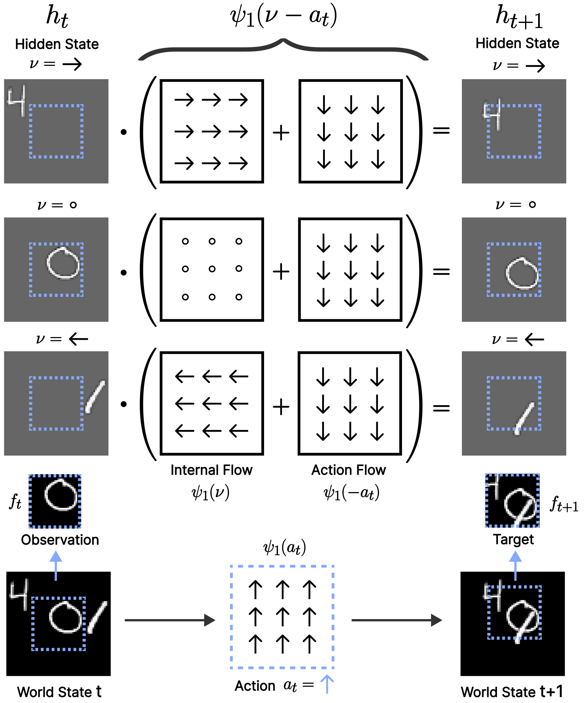
\end{equation}In the case when the action space is the 2D translation group (such as in our MNIST World experiments in the following section), the representation $`T_{a_t}`$ takes the form of another ‘Action Flow’ ($`\psi_1(-a_t)`$) describing the visual flow induced by the action in the agent’s reference frame. By the properties of flows, this then combines with the ‘Internal Flows’ ($`\psi_1(\nu)`$) of the ‘velocity channels’, yielding a simple combined flow, $`\psi_1(\nu - a_t)`$, in the recurrence. When the action space is more sophisticated, such as involving rotations, the representation acts directly on the spatial dimensions and velocity channels of the hidden state itself. In the following paragraphs we describe precisely how these abstract elements are instantiated for each of the datasets we explore in this study.
Instantiations for 2D / 3D Partially Observed Dynamic World Modeling
Simple Recurrent FloWM.
For the first set of experiments, to validate our framework in a 2D environment, we extend the model of with the unified self-motion equivariance introduced above (depicted in Figure [fig:2d_model_figure]). Explicitly, this yields the following recurrence:
\begin{equation}
\label{eqn:simple_flowm}
    h_{t+1}(\nu) = \psi_1(\nu - a_t) \cdot \sigma\bigl(\mathcal{W} \star h_t(\nu) + \mathrm{pad}(\hspace{0.4mm}\mathcal{U} \star f_t)\bigr),
\end{equation}where $`\mathcal{W} \star h_t`$, and $`\mathcal{U} \star f_t`$ denote convolutions over the hidden state and input spatial dimensions. To model partial observability, we simply write-in-to (denoted ‘$`\mathrm{pad(\cdot)}`$’), and read-out-from, a fixed $`\mathrm{window\_size} < \mathrm{world\_size}`$ portion of the hidden state (blue dashed square in Fig. [fig:2d_model_figure](a)), letting the rest of the hidden state flow around the agent’s field of view according to $`\psi_1(\nu - a_t)`$. In particular, the hidden state is windowed at each timestep, pixel-wise max-pooled over ‘velocity channels’ and passed through a decoder $`g_{\theta}`$ to predict the next observation, explicitly: $`\hat{f}_{t+1} = g_{\theta}\bigl(\max_\nu(\mathrm{window}(h_{t+1}))\bigr)`$. We see that this is equivalent to an instantiation of our general framework with $`\mathrm{E}_{\theta}[f_t; h_t](\nu) = \mathcal{U} \star f_t`$, and $`U_{\theta}[h_t; o_t] = \sigma(\mathcal{W} \star h_t + \mathrm{pad}(o_t))`$ where all operations are equivariant to translation, and thus satisfy the conditions of Equation [eqn:floweq_congs].
Transformer-Based FloWM.
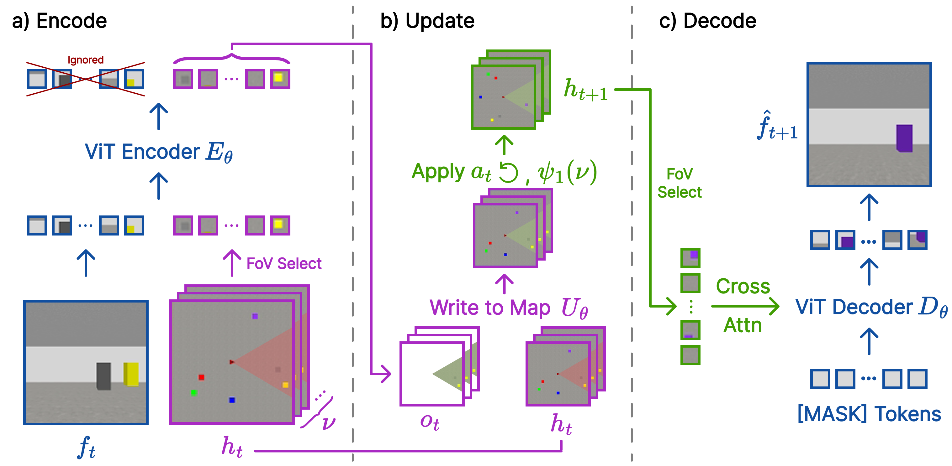
To extend our FloWM framework to work with more complex datasets, such as our second set of experiments involving a 3D world with other moving elements, we construct a second instantiation of the FloWM with a Vision Transformer (ViT) based encoder and decoder, depicted in Fig. 3 (note that it is still a recurrent model, but each step’s update computed with a transformer, rather than simple addition of liner maps). Specifically, in this setting $`h_t`$ is a set of spatially organized token embeddings that act as a group-structured latent map. In the spirit of , we set this map to be a ‘top-down’ 2D abstract version of the true 3-dimensional environment the agent inhabits. We denote this set of tokens $`h_t := \{\smash{h^{(x,y)}_t} | (x,y) \in [0, W) \times [0, H)\}`$ where $`(x,y)`$ are the spatial coordinates of the token. Most importantly, this map is group-structured with respect to the agent’s action group (2D translation and 90-degree rotation), and the group of external object motion (2D translation), giving us a known form of the representation of these group elements in the latent map, $`T_g`$.
The goal of the encoder $`\mathrm{E}_{\theta}[f_t;h_t]`$, instantiated as a ViT, is then to take the tokens of the map corresponding to the current field of view, and update them using the image patch tokens ($`\mathrm{patchify}(f_t)`$). Explicitly: $`\mathrm{E}_{\theta}[f_t; h_t] = \mathrm{ViT}[\mathrm{concat[}\mathrm{patchify}(f_t); \mathrm{FoV}(h_t)]] = o_t`$, where $`\mathrm{FoV}(h_t)`$ returns a fixed subset of $`{h_t}`$ corresponding to the 2D triangular wedge field of view of the agent, depicted in Fig. 3. We highlight that the coordinates of this set are fixed since the map is always egocentric, shifting and rotating around the agent in the center. The update operation $`\mathrm{U}_{\theta}[h_t; o_t]`$ then simply performs a gated combination of the output of the encoder (map token latent positions only), and the previous values of the hidden state $`\mathrm{FoV}(h_t)`$. Explicitly, matching our framework:
\begin{equation}
\mathrm{U}_{\theta}[h_t; o_t] ^{(x,y)} =
\begin{cases}
(1-\alpha) * h^{(x,y)}_t + \alpha * o_t^{(x,y)} & \text{if } x, y \in \text{FoV} \\
h^{(x,y)}_t & \text{otherwise} \\
\end{cases} ,
\end{equation}where $`\alpha = \sigma(\mathbf{W}\ \mathrm{concat}[h^{(x,y)}_t; o_t^{(x,y)}])`$ for some learnable gating weights $`\mathbf{W}`$. We can see that the update operation $`\mathrm{U}_{\theta}`$ is indeed equivariant with respect to shifts or rotations of the spatial coordinates of its inputs, satisfying equation [eqn:floweq_congs] for $`\mathrm{U}_{\theta}`$. However, since the encoder must map from the 3D first person point of view of the agent, to an abstract top-down map, it is highly non-trivial to make this transformation exactly action equivariant by design (without relying on explicit depth unprojection). Therefore, instead, we simply treat the output of the encoder as if it were equivariant in the recurrence relation, and anticipate that the transformation $`T_{a_t}^{-1} \psi_1(\nu)`$ between timesteps will encourage the encoder to learn to become equivariant, as has been demonstrated in prior work . As we will demonstrate empirically in the following section, in practice this appears to hold. We provide more model details in Appendix 13, and in Section 5 we review related models that have similarly structured representations with respect to self-motion, but may be seen as special cases of this framework without input-flow equivariance.
Experiments
In this section we present our 2D and 3D partially observable dynamic world modeling benchmarks, and compare the proposed FloWM framework against state-of-the-art video diffusion world models and ablations of our FloWM. Our results on these datasets validate that unified self-motion and external flow equivariance are useful for modeling dynamics out of the field of view, whereas current world model formulations struggle due to their lack of unified memory and inability to model dynamics naturally. Links to model and dataset code are available on the project website here .
Diffusion-based Baselines
Diffusion Forcing Transformer.
Due to its claims of long term consistency and flexible autoregressive inference, we chose History-guided Diffusion Forcing as the baseline training method, using latent diffusion with a CogVideoX-style transformer backbone, which we will call here DFoT . For each dataset, we first train a spatial downsampling VAE to encode video frames into a latent representation before being fed to diffusion model. Unlike FloWM recurrent models, and due to the diffusion forcing objective, during training for DFoT we make no distinction between observation and prediction frames, and train on fixed length sequences in the self-attention window. To condition on actions, we follow CogVideoX-style action conditioning, including the embedded action sequence in the self-attention window. During inference, we maintain context frames while denoising the prediction frames; the prediction frames begin at full noise and are gradually denoised until they are clean with the diffusion model, and then the sliding window advances by the number of predicted frames. More details, discussion, and training settings for DFoT can be found in Appendix 15.2.
Diffusion Forcing State Space Model.
As a representative comparative work on memory-augmented video diffusion models, we compare against a recently proposed approach that combines a short horizon Diffusion forcing transformer (for local consistency) with a blockwise scan State Space Model module (for long horizon memory) . This model employs the same VAE as DFoT across all datasets to operate in latent space. Differing from DFoT, there are some number of clean context frames during training, and the prediction frames are predicted according to the diffusion forcing objective, encouraging the model to leverage the clean context . During inference, we follow the same procedure as in DFoT, and refer to this model as DFoT-SSM. Further details are provided in Appendix 15.4.
2D MNIST World Benchmark
Dataset
To test our architecture on partially observable dynamic world modeling, we propose a simple MNIST World dataset. The world is a 2D black canvas with multiple MNIST digits moving at random constant velocities. The agent is provided a view of the world, smaller than the world size, yielding partial observability. At each discrete timestep, the world evolves according to the velocity of each object, and the agent takes a random action (relative ($`x`$, $`y`$) offset) to move its viewpoint. The edges roll, so a digit moving off the screen to the left will reappear on the right. Given 50 observation frames, the training task is to predict the dynamics played out for 20 future frames, integrating future self-motion (given) and world dynamics. To test length generalization, we additionally run inference with 50 observation rames and 150 prediction frames. We include ablations on data subsets with different combinations of partial observability, object dynamics, and self-motion in Appendix 12.
Results
On the MNIST World dataset, we train and evaluate the Simple Recurrent FloWM introduced in Section 3.2, which includes velocity channels (VC) and self-motion equivariance (SME). We also include ablations FloWM (no VC), FloWM (no VC, no SME), and the diffusion baselines mentioned above. We note here that FloWM (no VC, no SME) is just a simple convolutional RNN. More training and model details are available in Appendices 14 and 15.2. At each timestep, we calculate various quality metrics for the predicted frames for each model with respect to the ground truth, reported in Table [tab:mnistworld_metrics]. Example rollouts and full world view visualizations are available in Fig. 4(a).
Predictions from the FloWM remain consistent with the motion of objects out of its view for 150 timesteps past the observation window, well beyond its training prediction horizon of 20 timesteps, while FloWM (no VC, no SME) fails. We find that the FloWM (no VC) can still somewhat learn to model unobserved dynamics, especially within its training window, but drifts over time; length extrapolation abilities are presented in Fig. 4(b). We further find that models combining SME and VC require orders of magnitude less training steps to converge compared with those without these priors, shown in Fig. 4(c). The DFoT model’s predictions quickly diverge from the ground truth, even within its training window, just generating plausible digit-like artifacts. The DFoT-SSM model’s predictions show the digits slowly fading to black. Through additional results in Appendix 12, we explore how the DFoT model can sometimes handle partial observability, object dynamics, and self-motion individually, but not in any combination.
3D Dynamic Block World Benchmark
Dataset
Reasoning about the dynamics of the 3D world from 2D image observations requires approximating unprojection of egocentric views to a world-centric representation. To validate FloWM on this more difficult setting, we further introduce a simple 3D dataset, built in the Miniworld environment . An agent is spawned in a random position in a square room, along with colored blocks initialized with random positions and velocities. At each timestep, the blocks evolve according to their velocities, and the agent takes one of four discrete actions: turn left, turn right, move straight, or do nothing. The blocks bounce when encountering a wall, making the task of modeling dynamics out of view significantly harder. The data-generating agent follows a biased random exploration strategy, sometimes pausing to observe the room’s dynamics from next to the wall. Videos of the agent’s observations are collected; similar to the MNIST World setup, during training the world model is given 50 observation frames as context and must predict the dynamics evolving over the next 90 steps, given the agent’s actions. More details, including ablations involving a static version of Block World are included in Appendix 11, and more training details are available in Appendix 13.
Results
On the 3D Dynamic Block World dataset, we compare our Transformer-Based FloWM from Section 3.2 and Fig. 3 with the diffusion baseline, also including the ablations FloWM (no VC) and FloWM (no VC, no SME). We report the metrics on rollouts of 70 and 210 prediction frames, given 70 frames of context in Table [tab:blockworld_metrics_dynamic]1. Example rollouts are visualized in Figure 5 and on the website here . Similar to the 2D experiments, we observe the FloWM’s predictions are able to remain consistent for as many as 210 frames of future prediction, while the baselines and ablations are not. The average prediction error through time is represented in Figure 5, demonstrating FloWM’s consistent rollouts through long horizons. Perceptually, DFoT and SSM model predictions frequently hallucinate new objects and forget old ones, aligning with the hypothesis that their architectures are not well suited for partially observable dynamic environments. In addition to the standard, simpler 3D Dynamic Block World dataset, we evaluate our model and baselines on a significantly more visually difficult Textured 3D Dynamic Block World dataset, where block, wall, and floor textures are randomly assigned for each example. The same gap holds, demonstrating that FloWM is additionally applicable to more visually realistic settings. Results for this set are available in Appendix 11.
 />
/>
Related Work
Generative World Modeling with Memory.
As mentioned in Section 2, there have been a few prior works that augment diffusion video models to improve long horizon consistency and go beyond the limited context window of transformer-based diffusion models. Here, we will discuss the ones most relevant to this work in detail, and leave broader related work to Appendix 10. To begin, all work mentioned here focuses on static scenes only, and conditions on actions through token-based conditioning, lacking any way to harmoniously integrate the agent’s actions over time. The baseline DFoT-SSM model incorporates a recurrent SSM backbone for the purposes of long-context consistency and memory; however, the SSM is primarily remembering viewpoint-dependent observations, similar to extending the self-attention context window, and does not have any explicit computation steps for predicting the state of the world out of the view of the agent . As shown in our work, these drawbacks limit the ability for that class of model to perform accurate dynamics prediction. Another recently developed, separate model, WORLDMEM augments diffusion video models by placing past image observations in a memory bank for later retrieval based on the camera position . An existing ablation of their model in their paper involving camera view prediction may encourage the model to learn how to integrate its global position in time, similar to the effect of self-motion equivariance in our work, but their memory mechanism is fundamentally different, relying on self-attention to integrate information for self-consistency. Their retrieval mechanism also memorizes viewpoint variant information and would be ill suited for dynamic prediction. Recent work from maintains a 3d voxel map of the environment, later retrieved to condition diffusion generation. However, their method relies on depth unprojection, the voxels are updated via max pooling instead of a more flexible recurrence relation, and are prohibitively expensive for large hidden state sizes.
Equivariant World Modeling.
Perhaps most related to our proposed FloWM are world modeling frameworks with similarly structured ‘map’ memories. For example, Neural Map introduced a spatially organized 2D memory that stores observations at estimated agent coordinates. The storage location of these observations is shifted precisely according to the agent’s actions, yielding an effectively equivariant ‘allocentric’ latent map. In Section 5 of the paper, the authors describe an egocentric version of their model which can in fact be seen as a special case of our FloWM, specifically equivalent to the ablation without velocity channels. The authors demonstrate that their allocentric map enables long-term recall and generalization in navigation tasks. In a similar vein, EgoMap leverages inverse perspective transformations to map from observations in 3D environments to a top-down egocentric map. This work also explicitly transforms the latent map in an action-conditioned manner, although the transformation is learned with a Spatial Transformer Network, making it only approximately equivariant. Our work can be seen to formalize these early models in the framework of group theory, allowing us to extend the action space beyond just spatial translation to any Lie group and any world space. For example, our framework can theoretically support full 3-dimensional ‘neural maps’ without problem, following the framework of flow equivariance. Finally, there are a few other works that discuss equivariant world modeling, but are less precisely related to our own. Specifically, was one of the first works to build equivariant policy and value networks for reinforcement learning, but not with respect to motion, instead with respect to the symmetries of the environment (such as static rotations or translations). More recent work proposes to approach the goal of building equivariant world models in a more approximate manner by conditioning or encouraging equivariance through training losses, rather than our approach which builds it in explicitly.
Limitations & Future Work.
Our current instantiations of FloWM target environments where both the agent and objects undergo relatively simple, rigid motions under a known action parameterization. This setting lets us isolate the role of the flow equivariant memory under partial observability, but it does not yet capture richer non-rigid or semantic actions (e.g. articulated bodies, deforming objects, or discrete semantic actions such as “open door” or “pick up object”). Extending the flow equivariant recurrence to actions that live in more expressive latent groups or hierarchies, and to domains where agent actions are semantic rather than purely geometric, is an important direction for future work.
Our experiments also focus on deterministic dynamics given an action sequence, and we train FloWM with a single-step reconstruction loss to predict a single future rollout. We view the ability to model deterministic trajectories as a prerequisite to eventually model stochastic ones. The same flow equivariant latent map could in principle be combined with stochastic latent variables to enable stochastic dynamic prediction, representing another interesting line of future work.
Training and inference compute requirements for FloWM remain within the same order of magnitude as the strongest baselines despite maintaining a recurrent state. We report compute metrics and suggest several future directions to further improve efficiency in Appendix 16.
There are a few architectural limitations to note in this current study. As noted, our 3D FloWM ViT Encoder is not analytically equivariant with respect to 3D transformations. While the model appears to learn this equivariance over time, and therefore still benefits from the group-structured hidden state, we observe that this results in slower learning initially until a point where approximate equivariance appears learned, and the model can leverage the velocity channels properly. Future work that incorporates a proper analytically equivariant 3D encoder would likely observe significantly faster training speeds and lower loss, akin to the performance we report on the 2D dataset. Second, Flow Equivariance to date has only been developed with respect to discrete sets of flows $`V`$, while real world velocities may span a continuous range. However, prior work has repeatedly demonstrated empirically that even equivariance to small discretized groups yields performance improvements on data that is symmetric with respect to the full group . Recent theoretical work has further characterized the value of such ‘approximate’ or ‘partial’ group equivariance, demonstrating the value that such methods hold even if not exact . Future work to extend flow equivariance to continuous velocities would regardless still hold significant value. Lastly, our latent world map is egocentric and fixed in spatial extent and resolution. While the textured Block World results indicate that FloWM can handle increased visual complexity, scaling to more realistic, open world scenes will likely require variable sized maps and stronger perceptual backbones.
Finally, we believe a complementary line of work is to combine FloWM with insights from non-generative world models. In this paper, we refer to “embodied world models” as an egocentric sensory stream paired with self motion actions, and evaluate FloWM purely as a predictive video model. In the future, the flow equivariant latent memory that we introduce in this paper could be used as a representation backbone within a JEPA or TDMPC2 style world model to improve long horizon dynamics predictions . Together, they could represent a major step forward to tackle downstream embodied tasks such as autonomous driving, robotic manipulation, or game environments through planning over the model predictions or latent space.
Conclusion
In this work, we have introduced Flow Equivariant World Models, a new framework unifying both internally and externally generated motion for more accurate and efficient world modeling in partially observable settings with dynamic objects out of the agent’s view. Our results on both the 2D and 3D datasets with these properties demonstrate the potential of flow equivariance, and highlight the limitations with current state-of-the-art diffusion-based video world models. Specifically, we find that flow equivariant world models are able to represent motion in a structured symmetric manner, permitting faster learning, lower error, fewer hallucinations, and more stable rollouts far beyond the training length. We believe this work lays the theoretical groundwork along with empirical validation to support the potential for a novel symmetry-structured approach for efficient and effective world modeling.
Acknowledgments
The authors would like to thank Domas Buracas, Zhiyi Li, Nicklas Hansen, Nathan Cloos, Christian Shewmake, William Chung, and Kirill Dubovitskiy for their helpful discussion and feedback about early versions of this work. This work has been made possible in part by a gift from the Chan Zuckerberg Initiative Foundation to establish the Kempner Institute for the Study of Natural and Artificial Intelligence at Harvard University.
Generalized Flow Equivariance Proof
In this section, we prove by induction that the generalized Flow Equivariant Recurrence Relation of Equation [eqn:general_floweq] is indeed flow equivariant, following the proof technique of .
First, to restate the problem, we wish to show that for the recurrence defined as follows:
\begin{equation}
\label{eqn:general_floweq_app}
     h_{t+1}(\nu) = \psi_1(\nu) \cdot  \mathrm{U}_{\theta}\bigl[
    h_{t}(\nu);\  E_{\theta} \left[f_t, h_{t} \right](\nu)\bigr],
\end{equation}if we assume that:
-
The encoder satisfies the ‘trivial lift’ condition to the velocity field: $`E_{\theta} \left[f_t; h_t \right](\nu) = E_{\theta} \left[f_t; h_t \right](\hat{\nu}) \ \ \forall \nu, \hat{\nu} \in \mathfrak{g}`$
-
The encoder and decoder are both group equivariant with respect to their arguments: $`\mathrm{E}_{\theta}\left[g \cdot f_t;\ g \cdot h_t\right] = g \cdot \mathrm{E}_{\theta}\left[f_t ;h_t\right] \quad \& \quad \mathrm{U}_{\theta}\left[g \cdot h_t;\ g \cdot o_t \right] = g \cdot \mathrm{U}_{\theta}\left[h_t;\ o_t\right]`$
-
The hidden state is initialized to be constant along the flow dimension and invariant to the flow action: $`h_0(\nu) = h_0(\nu')\ \forall\, \nu', \nu \in V`$ and $`\psi_1(\nu) \cdot h_0(\nu) = h_0(\nu) \ \forall \,\nu \in V,`$
then, the follow flow equivariance commutation relation holds:
\begin{equation}
 \label{eqn:defn_flow_action_app}
     h_t[\psi(\hat{\nu}) \cdot f] (\nu) =  \psi_{t}(\hat{\nu}) \cdot h_t[f](\nu- \hat{\nu})\ \ \forall t.
\end{equation}Let $`h[f] \in {\mathcal{F}}_{K'}(Y, {\mathbb{Z}})`$ be a the output of the generalized flow equivariant recurrence relation as defined in Equation [eqn:general_floweq_app], with hidden-state initialization invariant to the group action and constant in the flow dimension, i.e. $`h_0(\nu, g) = h_0(\nu',g)\ \forall\, \nu', \nu \in V`$ and $`\psi_1(\nu) \cdot h_0(\nu, g) = h_0(\nu, g) \ \forall \,\nu \in V,\,g\in G`$. Then, $`h[f]`$ is flow equivariant with the following representation of the action of the flow in the output space for $`t \geq 1`$:
\begin{equation}
     (\psi(\hat{\nu}) \cdot h[f])_t(\nu, g) = h_t[f](\nu - \hat{\nu}, \psi_{t}(\hat{\nu})^{-1} \cdot g)
\end{equation}We note for the sake of completeness, that this then implies the following equivariance relations:
\begin{equation}
     h_t[\psi(\hat{\nu}) \cdot f](\nu, g) = h_t[f](\nu - \hat{\nu}, \psi_{t}(\hat{\nu})^{-1} \cdot g) = \psi_{t}(\hat{\nu}) \cdot h_t[f](\nu - \hat{\nu}, g)
\end{equation}Furthermore, in all settings in this work, $`G`$ refers to the 2D translation group, either indexing pixel coordinates (MNIST), or 2D latent map coordinates (Block world) referred to as $`(x,y)`$ in the main text.
We see that, different from the work of , since the generalized recurrence relation in Eqn. [eqn:general_floweq_app] applies the flow update after the input has been combined with the hidden state (i.e. outside the $`\mathrm{U}_{\theta}`$ operator), the commutation relation in Eqn. [eqn:defn_flow_action_app] now has a $`t`$ index on $`\psi_t`$, instead of $`t-1`$ as written in equation [eqn:defn_flow_action].
Proof. (Theorem, Generalized Flow Equivariance)
Base Case: The base case is trivially true from the initial condition:
\begin{align}
    h_0[\psi(\hat{\nu}) \cdot f_{<0}](\nu, g) & =  h_0[ f_{<0}](\nu, g) \quad \text{(by initial cond. being independent of input)}\\
    & = h_0[f_{<0}](\nu - \hat{\nu}, \psi_{t}(\hat{\nu})^{-1} \cdot g) \quad \text{(by constant init.)}
\end{align}Inductive Step: Assuming $`h_t[\psi(\hat{\nu}) \cdot f](\nu, g) = \psi_{t}(\hat{\nu}) \cdot h_t[f](\nu - \hat{\nu}, g) \, \forall\, \nu \in V, g \in G`$, for some $`t \geq 0`$, we wish to prove this also holds for $`t+1`$:
Using the Generalized Flow Recurrence (Eqn. [eqn:general_floweq_app]) on the transformed input, we get:
\begin{align}
h_{t+1}[\psi(\hat\nu)\!\cdot\! f](\nu,g)
&=\psi_{1}(\nu)\!\cdot\!
      \mathrm{U}_{\theta}\!\Bigl(
        h_{t}[\psi(\hat\nu)\!\cdot\! f](\nu,g)\ ;\
        \mathrm{E}_{\theta}\!\left[(\psi_{t}(\hat\nu)\!\cdot\! f_t),\ h_{t}[\psi(\hat\nu)\!\cdot\! f]\right]\!(\nu)
      \Bigr)
\\[2mm]
\text{(by inductive hyp.)}\quad
&=\psi_{1}(\nu)\!\cdot\!
      \mathrm{U}_{\theta}\!\Bigl(
        \psi_{t}(\hat{\nu}) \cdot h_t[f](\nu - \hat{\nu}, g)\ ;\
        \mathrm{E}_{\theta}\!\left[(\psi_{t}(\hat\nu)\!\cdot\! f_t),\ \psi(\hat\nu)_{t}\!\cdot\!h_{t}[f]\right]\!(\nu)
      \Bigr)
\\[2mm]
\text{(trivial lift in $\nu$)}\quad
&=\psi_{1}(\nu)\!\cdot\!
      \mathrm{U}_{\theta}\!\Bigl(
        \psi_{t}(\hat{\nu}) \cdot h_t[f](\nu - \hat{\nu}, g)\ ;\
        \mathrm{E}_{\theta}\!\left[(\psi_{t}(\hat\nu)\!\cdot\! f_t),\ \psi(\hat\nu)_{t}\!\cdot\!h_{t}[f]\right]\!(\nu-\hat\nu)
      \Bigr)
\\[2mm]
\text{(equivariance of $E_\theta$)}\quad
&=\psi_{1}(\nu)\!\cdot\!
      \mathrm{U}_{\theta}\!\Bigl(
        \psi_{t}(\hat{\nu}) \cdot h_t[f](\nu - \hat{\nu}, g)\ ;\
        \psi_{t}(\hat\nu)\!\cdot\!
        \mathrm{E}_{\theta}\!\left[f_t,\ h_{t}[f]\right]\!(\nu-\hat\nu)
      \Bigr)
\\[2mm]
%
\text{(equivariance of $U_\theta$)}\quad
&=\psi_{1}(\nu)\!\cdot\!
      \psi_{t}(\hat\nu)\!\cdot\!
      \mathrm{U}_{\theta}\!\Bigl(
        h_{t}[f](\nu-\hat\nu,g)\ ;\
        \mathrm{E}_{\theta}\!\left[f_t,\ h_{t}[f]\right]\!(\nu-\hat\nu)
      \Bigr)
\\[2mm]
\text{(flow composition)}\quad
&=\psi_{t+1}(\hat\nu)\!\cdot\!
   \psi_{1}(\nu-\hat\nu)\!\cdot\!
      \mathrm{U}_{\theta}\!\Bigl(
        h_{t}[f](\nu-\hat\nu,g)\ ;\
        \mathrm{E}_{\theta}\!\left[f_t,\ h_{t}[f]\right]\!(\nu-\hat\nu)
      \Bigr)
\\[2mm]
\text{(by Eqn. \ref{eqn:general_floweq_app})}\quad
&=\psi_{t+1}(\hat\nu)\!\cdot\! h_{t+1}[f](\nu-\hat\nu,g)
\\[2mm]
&=h_{t+1}[f]\bigl(\nu-\hat\nu,\;\psi_{t+1}(\hat\nu)^{-1}\!\cdot g\bigr).
\end{align}Thus, assuming the inductive hypothesis for time $`t`$ implies the desired relation at time $`t+1`$; together with the base case this completes the induction and proves the Theorem. ◻
Additional Related Work
World Models
World modeling is commonly framed as learning to predict how an environment evolves over time, conditioned on an agent’s actions, enabling “imagination” for data-efficient policy learning and model-based planning . Recent progress in large scale generative modeling has extended this paradigm to video prediction, yielding generative world models that directly predict future observations in pixel or latent video space . When successful, these models capture both the stochasticity and multimodality of environment dynamics, and can be queried to simulate counterfactual futures under different action sequences. Our work also falls in this category; the prediction target is the agent’s visual observations. However, we focus on the regime where accurate prediction requires persistent memory of scene state across long horizons and changing viewpoints.
A dominant current approach to generative world modeling uses transformer backbones trained with diffusion-style objectives, extending to long rollouts via sliding window inference . In particular, History-Guided Diffusion Forcing, which extends video diffusion to stable autoregressive rollouts, denoises multiple frames jointly and can leverage attention over recent context to improve short-range temporal coherence and conditioning fidelity (represented in the DFoT baseline we benchmark against) . However, in partially observed settings, long horizon prediction requires retrieving and updating information that may have been observed far in the past (e.g. objects that moved out of view). Under the common sliding window attention regime, context is necessarily truncated as rollouts grow, so information that leaves the window becomes inaccessible to the model to generate new frames. The model must remain consistent with past observations while simultaneously reflecting state changes that occurred out of view, yet neither requirement is naturally supported once the relevant evidence is outside the attention window (as visualized in Figure 2). Consequently, despite strong perceptual quality, windowed diffusion transformer simulators struggle to maintain globally consistent, stateful predictions over long horizons, especially in scenes that have out of view dynamics.
In contrast, many non-generative world models learn compact latent dynamics tailored for control rather than reconstructing future observations. Representative approaches such as TDMPC2 and V-JEPA style predictive learning maintain recurrent latent state and optimize objectives that encourage predictability and useful abstractions for downstream decision making . These methods can be highly effective for planning in continuous control, but they typically do not aim to produce observation space rollouts, and their benchmarks and objectives often place less emphasis on long horizon, out-of-view state tracking in visually rich, partially observed environments. This gap leads to the question we put forward in this work: how to build an action-consistent world model with a persistent state that can stably represent and evolve both self-motion and external object motion over hundreds of steps, enabling accurate prediction even when the relevant dynamics occur outside the current field of view.
Memory in generative world models
Local temporal consistency in generative world models can often be maintained using self attention over recent history (e.g. through the history guided diffusion forcing scheme mentioned in the previous paragraph), but this mechanism degrades once rollouts exceed the model’s effective attention window. The comprehensive history of past observations cannot all be kept in context; though there is significant work on long context extensions, such as sparse attention or compression techniques, we believe that more principled solutions are needed to represent the world properly . In partially observed environments (which we argue all realistic environments eventually are), long horizon prediction requires a persistent and updateable state that can carry information forward even when relevant evidence is no longer in-context. Tracking objects that move out of view and continuing to evolve their state according to previously observed dynamics is an example of this. A growing set of methods therefore augment transformer backbones with explicit memory, yet many existing proposals either (i) primarily address static scene consistency, (ii) store viewpoint-variant observations rather than a world-centric state, or (iii) introduce memory structures whose capacity or cost scales poorly with horizon.
One representative design (and the baseline we chose in our experiments) combines a local attention window for short-range coherence with an auxiliary SSM memory module that compresses past observations . While such hybrids can stabilize generation over modest horizons, in practice we observed they often learn to memorize camera-conditioned appearance rather than maintaining a canonical scene state. This viewpoint-variant storage becomes brittle under viewpoint changes and especially under dynamics that evolve out of view, since the memory must simultaneously (a) retain evidence from past viewpoints and (b) support correct state updates when the scene changes without direct observation. Moreover, when the auxiliary module has limited functional capacity (e.g. linear state updates), it can further constrain the complexity of dynamics and viewpoint variation that can be retained over long horizons.
Other memory strategies trade compression for retrieval. For instance, database-style approaches such as WORLDMEM store past frames (or features) and retrieve relevant context based on field-of-view overlap . While retrieval can recover visually similar evidence, storing raw viewpoints can be inadequate for dynamic environments where the correct future state may differ from any previously observed frame. Furthermore, the memory footprint typically grows with the number of observations unless aggressive pruning or summarization is introduced.
A third class maintains explicit geometric memory, such as pointcloud or voxel-based representations. These representations can promote viewpoint invariant consistency, but they are expensive to maintain at scale . Further, a recent method that separates dynamic from static only remembers the static portion through its pointcloud memory; the dynamic portion is generated anew, conditioned on local frames, so it is unable to handle out of view dynamics well . More generally, many existing 3D memory constructions are designed for view synthesis with largely static memory, making it challenging to represent and update long horizon dynamics under partial observability. Together, these limitations motivate memory mechanisms that are explicitly world-centric, consistent with action conditioning, and dynamically updateable over long horizons.
An additional intuition figure for partially observable dynamic world modeling in 2d environments (such as our MNIST World benchmark) is available in Figure 6.
Novel View Synthesis and 3D Priors
A separate line of work in novel view synthesis and 3D reconstruction, such as NeRFs and 3D Gaussian Splatting, focuses on building explicit scene representations that enable photorealistic rendering from new camera poses . These methods provide strong geometric and multi-view priors, often yielding impressive viewpoint consistency because rendering is mediated by an underlying 3D representation rather than purely by autoregressive appearance modeling. Extensions to dynamic settings (e.g. “4D” variants that model time varying geometry or appearance) further support rerendering observed motions from novel viewpoints . However, these approaches are typically formulated as reconstruction or retargeted rendering problems conditioned on observed frames, rather than as action-conditioned future prediction under partial observability. In other words, they are primarily designed to visualize or interpolate dynamics that are present in the captured data, not to predict how an environment will evolve forward in time when key parts of the state may be unobserved and must be remembered and updated. Further, their representations are often not semantic, so they cannot be used to learn generalized prediction models over future states of the world.
World model evaluation on long horizon memory and dynamics
Evaluation of generative world models is often centered on perceptual similarity and sample quality using metrics such as PSNR, SSIM, and distributional scores like FVD . While useful, these metrics can underemphasize the specific failure modes that arise in long horizon, partially observed prediction: a model may remain visually plausible yet drift in state consistency, forget out-of-view objects, hallucinate new objects, or violate deterministic dynamics in ways that are not strongly penalized by short horizon or ambiguity-tolerant benchmarks. In this work we therefore target a more diagnostic regime: deterministic dynamics under controlled partial observability, where the correct future is well defined and errors can be attributed to deficiencies in memory and state tracking rather than to inherent stochasticity. We view deterministic dynamics modeling as a first step in modeling all classes of dynamics properly, since it is a subset of more general stochastic dynamics. Concretely, we contribute a controlled dataset and protocol that determines whether a world model can (i) retain information beyond a local context window, (ii) update its hidden state when dynamics evolve out of view, and (iii) maintain viewpoint-consistent predictions that reflect an underlying world centric state over long horizons.
Equivariant World Models
Equivariant models respect the symmetry of their data, ensuring that structured transformations in the input induce predictable changes in the model’s internal state. This inductive bias has indeed been found to be valuable in prior work on world modeling. Specifically, although not explicitly framed as equivariant, one of the most related world modeling architectures to our proposed self-motion equivariance is the Neural Map . This work introduced a spatially organized 2D memory that stores observations at estimated agent coordinates. The storage location of these observations is shifted precisely according to the agent’s actions, yielding an effectively equivariant “allocentric” latent map. In Section 5 of the paper, the authors describe an egocentric version of their model which can in fact be seen as a special case of our FloWM, specifically equivalent to the ablation without velocity channels. The authors demonstrate that their allocentric map enables long-term recall and generalization in navigation tasks. In a similar vein, EgoMap built on this by leveraging inverse perspective transformations to map from observations in 3D environments to a top-down egocentric map. This work also explicitly transforms the latent map in an action-conditioned manner, although the transformation is learned with a Spatial Transformer Network, making it only approximately equivariant. Our work can be seen to formalize these early models in the framework of group theory, allowing us to extend the action space beyond just spatial translation to any Lie group and any world space. For example, our framework can theoretically support full 3-dimensional ‘neural maps’ without problem, following the framework of flow equivariance. Finally, there are a few other works that discuss equivariant world modeling, but are less precisely related to our own. Specifically, was one of the first works to build equivariant policy and value networks for reinforcement learning, but not with respect to motion, instead with respect to the symmetries of the environment (such as static rotations or translations). More recent work proposes to approach the goal of building equivariant world models in a more approximate manner by conditioning or encouraging equivariance through training losses, rather than our approach which builds it in explicitly. Overall, we find all of these approaches to be complementary to our own and are excited for their combined potential.
Neuroscience.
Excitingly, in the neuroscience literature, there is evidence for predictive processing in the mammalian visual system which is a function of self-motion signals. For example, and have found that responses in visual cortex are strongly modulated by self-motion signals, and mismatch between predicted and experienced stimuli. Similarly, it is known that position coding in the hippocampus through place cells and grid cells forms an equivariant map through phase coding of agent location. Explicitly, the phase of a given place cell’s spike shifts equivariantly with respect to the agent’s forward motion along a linear track. Further computational and theoretical work has demonstrated that grid-like activations emerge automatically through the enforcement of equivariance in cell responses . We believe this work suggests that there may indeed be a biological mechanism for encouraging the visual system to be a G-equivariant map from stimuli to a type of latent G-space.
Block World Additional Dataset Details and Results
Block World Dataset Details
Here, we describe dataset generation and parameter settings for the
Dynamic (presented in the main text), Textured Dynamic, and Static
subsets of Block World. The dataset generation parameters are described
in Table
1. Each dataset
example has a video of shape [num_frames, channels, height, width],
where channels is 3 for RGB; and an accompanying actions list of shape
[num_frames], for the discrete actions taken by the agent: left,
right, forward, or do nothing. Left and right correspond to a 90 degree
rotation such that the agent stays aligned with the grid. Each dataset
subset contains 10,000 videos for training, and 1,000 videos for
validation. The world size describes the number of coordinates in the
world able to be occupied by the agent or a block. The agent is spawned
in a random location within the world.
The Dynamic Block World dataset subset has blocks with randomized colors chosen from among blue, green, yellow, red, purple, and gray. There are no collisions between the blocks, or between the agent and the blocks, but the blocks bounce off the wall and change direction, making the motion nonlinear.
The textured dataset has the same dynamics behavior as the Dynamic Block World dataset, but with the following randomizations: (i) textures are randomized for the wall, chosen between brick, dark wood panel, wood panel; (ii) textures are randomized for the floor, chosen between cardboard, grass, concrete; (iii) textures are randomized for the blocks, chosen between metal grill, airduct grate, cinder blocks, and ceiling tiles; they remain colored randomly; (iv) 1/3 of the time, the object is a sphere instead of a block. In combination, these all add significant visual complexity and randomness to the environment.
The static subset just has the velocity of the objects initialized to 0; the agent’s exploration pattern is the same. We used Miniworld for this environment, and would like to thank the authors and contributors of Miniworld for creating a flexible and useful 3d simulator environment for agents .
| Data Subset | |||||||
| Size | |||||||
| Resolution | # Blocks | ||||||
| Range, x and y | |||||||
| Static Block World | 15x15 | 128x128 | 6-10 | 0 | |||
| Dynamic Block World | 15x15 | 128x128 | 6-10 | -1 to +1 (no diagonals) | |||
| Textured Dynamic Block World | 15x15 | 128x128 | 6-10 | -1 to +1 (no diagonals) |
Generation parameters for Block World dataset subsets.
Textured Block World Results
In this section we report additional results on the Textured Dynamic Block World dataset described above. The focus of this work is on the introduction of the flow equivariant framework for modeling partially observable dynamics, rather than the strength of the visual encoder / decoder. However the fact that FloWM can retain its performance improvements over the baselines in this settings suggests it can serve as a step forward for a general framework capable of encoding visually realistic scenes as well.
The results are available in Table [tab:textured_blockworld_results]. Example rollouts are visible on the project website here . Frames of the rollouts are visible in Figure 7. The metric numbers are not easily comparable to the other dataset split due to the different dataset statistics, but the relative distance is still clearly noticeable. We evaluate with 70 context frames to match the training regime of DFoT-SSM; more details are available in Appendix 15.4,
Static Block World Results
In this section we report additional results on the static Block World dataset described above. Results are available in Table [tab:blockworld_metrics_static]. As with the static MNIST World dataset, in this setting, the default configuration of FloWM with velocity channels only adds noise to the model, since the velocity channels have no external motion to model. Therefore, it is unsurprising that the FloWM (no VC) achieves the best metric scores. Despite the environment being static, DFoT and DFoT-SSM still struggle with keeping consistent with information that may have left their immediate context window. We hypothesize that due to the baseline models’ lack of a spatial memory, combined with the randomized number of blocks per environment, these models are unable to consistently remember where the blocks are. Here we also evaluate with 70 context frames to match the training regime of DFoT-SSM; more details are available in Appendix 15.4,
MNIST World Additional Dataset Details and Results
MNIST World Dataset Details
| Data Subset | Self-Motion | Dynamics | Partially Observable |
|---|---|---|---|
dynamic_fo_no_sm |
No | Yes | No |
dynamic_fo |
Yes | Yes | No |
static_po |
Yes | No | Yes |
dynamic_po |
Yes | Yes | Yes |
MNIST world data subsets demonstrating scaling difficulty in self-motion, dynamics, and partial observability.
Here, we describe dataset generation and parameter settings for our
ablations on self-motion, dynamics, and partial observability in the
MNIST World setting. The subsets are succinctly described in Table
2, and the generation
parameters in Table
3. A subset is described as
partially observable if the world size is larger than the window size.
We also scale the number of digits by the size of the world. Each
dataset example has a video of shape
[num_frames, channels, height, width], where channels is 1; and an
accompanying actions list of shape [num_frames, 2], for the x and y
translation of the agent view at each timestep. The dynamic_fo_no_sm
subset just has dynamics and is fully observable; the dynamic_fo
subset has dynamics and is fully observable, but also has self-motion;
the static_po subset is partially observable, and the agent has
self-motion, but the digits do not move; and finally, the dynamic_po
subset includes partial observability, agent movement, and dynamics. In
the main text, we report all results on just the dynamic_po subset.
For all subsets with dynamics, each digit is given an integer velocity
for x and y in the digit velocity range (e.g., -2 to 2). For each
dataset subset with self-motion, at each step during the observation and
prediction phase, a random integer is chosen in x and y to be the
agent’s view translation, bounded by the self-motion range (e.g., -10 to
10). For each dataset, objects that move across the boundary reappear on
the other side as a circular pad. Each dataset subset contains 180,000
videos in the training set, and 8,000 videos in the validation set.
Results on each of these data subsets for FloWM and baseline models are
described below.
| Data Subset | |||||||
| Size | |||||||
| Size | # Digits | ||||||
| Range | |||||||
| Range, x and y | |||||||
dynamic_fo_no_sm |
32 | 32 | 3 | 0 | -2 to +2 | ||
dynamic_fo |
32 | 32 | 3 | 10 | -2 to +2 | ||
static_po |
50 | 32 | 5 | 10 | 0 | ||
dynamic_po |
50 | 32 | 5 | 10 | -2 to +2 |
Generation parameters for MNIST World dataset subsets.
MNIST World Additional Results
Here we report additional results on the MNIST World subsets described above. We evaluate FloWM and FloWM ablations described in Appendix 14. We compare to the DFoT and DFoT-SSM baselines as described in Appendix 15.4.
The error (MSE) between the predicted future observations (rollout) and the ground truth is plotted for each baseline in Figure 8 as a function of forward prediction timestep (x-axis). Metrics are reported over the first 20 timesteps (the training length) and over the full 150 timesteps (length generalization) in Tables [tab:mnistworld_metrics_dynamic_fo_no_sm], [tab:mnistworld_metrics_dynamic_fo], [tab:mnistworld_metrics_static_po]. Due to being constructed with a different number of digits, metrics between the data subsets are not necessarily directly comparable. We provide the All-Black Baseline (model that only predicts 0 for future observations) as a form of normalization for comparison.
All models are able to do reasonably well on the simplest fully
observable dataset with no self-motion; note here the DFoT is doing
latent diffusion, so there is a small amount of error error from the
decoding step, contributing a baseline MSE of around 0.02, see Appendix
15.5 for more details. This setup
aligns with the typical setting of world modeling, where the information
that the model needs is expected to be in the attention window. The
other dataset splits do not follow this assumption, and the results
align with expectations about the model’s capabilities. The DFoT does
relatively better on the static static_po compared to the dynamic_po
dataset, due to not having to model dynamics, but the model’s outputs
still diverge from the ground truth quickly.
For a dataset where the velocity channels are redundant, i.e.
static_po, the FloWM (no VC) does slightly better than FloWM. Further
note that the FloWM (no VC) is able to have low error on most of the
tasks, though with a much higher value than FloWM as errors accumulate
due to not having the velocity channels to encode flow equivariantly.
Taken together, the ablations suggest that self-motion equivariance is
key to solving the problem, and that input flow equivariance via
velocity channels helps with exactness and convergence time, with the
tradeoff of a larger hidden state activation size.
FloWM Experiment Details: 3D Dynamic Block World
On the 3D Dynamic Block World Dataset, FloWM is built with 6-layer ViT encoders and decoders with 8 attention heads per layer, and an embedding dimension of 256.
Recurrence
The hidden state $`h_t \in \mathbb{R}^{|V| \times C_{hid} \times H_{world} \times W_{world}}`$ has $`|V|`$ velocity channels (indexed by the elements $`\nu \in V`$), and $`C_{hid}=256`$ hidden state channels (the same as the ViT token embedding dimension). The spatial dimensions of the hidden state are set to two times the world size for each dataset, meaning $`H_{world} = W_{world} = 32`$, so that the agent can be robust to being spawned anywhere. The hidden state is initialized to all zeros for the first timestep, i.e. $`h_0 = \mathbf{0}`$.
Velocity Channels
On the 3D Block World dataset, we add velocity channels only up to $`\pm 1`$ in both the X and Y dimensions of the map with no diagonal velocities, and include a zero velocity channel. Thus in total, $`|V| = 5`$ for the FloWM. Each channel is flowed by its corresponding velocity field, denoted by $`\psi_1(\nu) \cdot h_t(\nu)`$ for each of the velocities $`\nu`$, matching the velocity of the blocks in the real environment.
The actions of the agent then induce an additional flow of the hidden state, which we implement via the inverse of the representation of the action $`T_{-a_t} = T^{-1}_{a_t}`$. In practice, this is implemented by performing a $`\mathrm{roll}`$ operation on the hidden state by exactly 1 element for a forward action, and a $`+/-`$ 90-degree rotation for left or right actions respectively. Doing so allows the model’s representation of the world to stay accurate with respect to the transformation it has just done. Intuitively, if an agent has a representation of an object in front of it, then turns to the left, the world should shift to the right, opposite of the movement of the turn.
Transformer Details
The ViT Encoder takes in both image input tokens and the FoV-selected map latent tokens, and processes them together in the self-attention window. We use a patch size of 16 to patchify the image before a sin-cos absolute position embedding is added . The map latent tokens are also added together with a sin-cos absolute position embedding based on the position in the 2d map. Notably, these two are different embeddings and represent different spatial coordinates, one is of the image patch location, and the other is of the world location relative to the agent.
The ViT Decoder starts with a copy of a learnable $`\mathrm{[MASK]}`$ token at each patch location in the image, added with position embeddings representing the patch location in pixel space. Then it uses cross attention between the selected tokens in the Field of View of the updated hidden state $`\mathrm{FoV}(h_{t+1})`$ to make a prediction of the observation at the next timestep, $`\hat f_{t+1}`$.
Training Loss Details
To train FloWM, as well as the ablated versions, we provide the model with 50 observation frames as input, and train the model to predict the next 90 observations conditioned on the corresponding future action sequence. Specifically, we minimize the mean squared error (MSE) between the output of the model and the ground truth sequence, averaged over the prediction frames 50 to 139:
\begin{equation}
\mathcal{L}_{MSE} = \frac{1}{90}\sum_{t=50}^{139}||f_t - \hat{f}_t||^2_2.
\end{equation}The models are trained with the Adam optimizer with a learning rate of $`1e-4`$, a batch size of $`16`$. We use a teacher forcing ratio of $`12.5\%`$. They are each trained for 150k steps, or until converged. More details are available in Table 4.
| Component | Option | Value |
|---|---|---|
| Training | Learning rate | 1e-4 |
| Effective batch size | 16 | |
| Training steps | 150k | |
| GPU usage | 2$`\times`$H100 | |
| Teacher Forcing | 0.125 | |
| Model | Hidden channels | 256 |
| Encoder depth | 6 | |
| Encoder heads | 8 | |
| Decoder dim | 256 | |
| Decoder depth | 6 | |
| Decoder heads | 8 | |
| Patch size | 16 | |
| N Params | 10M | |
| Patch size | 16 |
Block World ViT FloWM Configurations.
FloWM Experiment Details: MNIST World
The Simple Recurrent version of the Flow Equivariant World Model for 2d settings is built as a simple sequence-to-sequence RNN with small CNN encoders/decoders to model MNIST digit features. Full code is available on the project page.
For completeness, we repeat the Simple Recurrent FloWM recurrence relation below:
\begin{equation}
% \label{eqn:self-motion}
    h_{t+1}(\nu) = \sigma\bigl(\psi_1(\nu - a_t) \cdot\mathcal{W} \star h_t(\nu) + \mathrm{pad}(\mathcal{U} \star f_t)\bigr).
\end{equation}Recurrence
The hidden state $`h_t \in \mathbb{R}^{|V| \times C_{hid} \times H_{world} \times W_{world}}`$ has $`|V|`$ velocity channels (indexed by the elements $`\nu \in V`$), and $`C_{hid}=64`$ hidden state channels. The spatial dimensions of the hidden state are set to match the world size for each dataset. For the partially observed world, this means $`H_{world} = W_{world} = 50`$ (where the window size is set to $`32 \times 32`$), while for the fully observed world, $`H_{world} = W_{world} = 32`$. The hidden state is initialized to all zeros for the first timestep, i.e. $`h_0 = \mathbf{0}`$.
The hidden state is processed between timesteps by a convolutional kernel $`\mathcal{W}`$. This kernel has the potential to span between velocity channels, and therefore model acceleration or more complex dynamics than static velocities. In this work, since our dataset has no such dynamics (we only have constant object velocities), we safely ignore the inter-velocity convolution terms, and simply set $`\mathcal{W}`$ to be a $`3 \times 3`$ convolutional kernel, with 64 input and output channels, circular padding, and no bias. We refer the interested reader to for details on the form of the full flow-equivariant convolution that could be equally used in this model. The hidden state is finally passed through a non-linearity $`\sigma`$ to complete the update to the next timestep. In this work, for MNIST World, we use a ReLU.
Velocity Channels
In this work, for MNIST World, we add velocity channels up to $`\pm 2`$ in both the X and Y dimensions of the image. Explicitly, $`V = \{(-2, -2), (-2, -1), \ldots (0, 0) \ldots (2,2)\}`$. Thus in total, $`|V| = 25`$ for the FloWM. Each channel is flowed by its corresponding velocity field (defined by $`\psi(\nu)`$) at each step. This is denoted by $`\psi_1(\nu) \cdot h_t(\nu)`$.
The actions of the agent then induce an additional flow of the visual stimulus. In order to be equivariant with respect to this flow in addition to the flows in $`V`$, we simply additionally flow each hidden state by the corresponding inverse of the action flow $`\psi(-a_t)`$. In total this gives the combined flow for each flow channel $`\psi_1(\nu - a_t)`$. In practice, this is implemented by performing a $`\mathrm{roll}`$ operation on the hidden state by exactly ($`\nu - a_t`$) pixels.
Encoder
The ‘encoder’ is simply a single convolutional layer, with $`3 \times 3`$ kernel $`\mathcal{U}`$, 1 input channel, and 64 output channels. The convolution uses circular padding, and no bias. The observation at timestep $`t`$ ($`f_t`$), is thus processed by the encoder ($`\mathcal{U} \star f_t`$) yielding the processed observation of the agent. Given this observation is only a partial observation of the full world, we must pad this observation to match the world size, and the size of the hidden state. We denote this operation as ‘$`\mathrm{pad}`$’ in the recurrence relation, and simply pad the boundary of the output of the encoder with $`0`$ to match the world-size (size of the hidden state).
Decoder
We learn the parameters of the FloWM by training it to predict future observations from its hidden state and the corresponding sequence of future actions. To compute this prediction, we take a consistent $`\mathrm{window\_size}`$ crop from the center of the hidden state, corresponding to the same location where the encoder ‘writes-in’. We denote this crop $`\mathrm{window}(h_{t+1})`$. To then enable the model to predict each pixel’s velocity independently, we perform a pixel-wise max-pool over the $`V`$ dimension (‘velocity channels’) before passing the result to a decoder $`g_{\theta}`$. Specifically: $`\hat{f}_{t+1} = g_{\theta}\bigl(\underset{\nu}{\max}\left(\mathrm{window}(h_{t+1})\right)\bigr)`$. The decoder $`g_{\theta}`$ is a simple 2 layer convolutional neural network with $`3 \times 3`$ convolutional kernels, 64 hidden channels, and a ReLU non-linearity between the layers.
Ablation: No Velocity Channels
To construct the ablated version of the FloWM with no velocity channels, we simply set $`V = \{(0,0)\}`$. Since the original FloWM model simply max-pools over velocity channels, the decoder already only takes a single velocity channel as input, so no other portions of the model need to change. We note that this model is identical to a simple convolutional recurrent neural network with self-motion equivariance. Explicitly:
\begin{equation}
h_{t+1} = \sigma\bigl(\psi_1(-a_t) \cdot\mathcal{W} \star h_t + \mathrm{pad}(\mathcal{U} \star f_t)\bigr).
\end{equation}Ablation: No Self-Motion Equivariance
To construct the ablated version of the FloWM with no self-motion equivariance, we simply remove the term $`-a_t`$ from the flow of the recurrence relation. Explicitly:
\begin{equation}
h_{t+1}(\nu) = \sigma\bigl(\psi_1(\nu) \cdot\mathcal{W} \star h_t(\nu) + \mathrm{pad}(\mathcal{U} \star f_t)\bigr).
\end{equation}We note that this is equivalent to the original FERNN model with the addition of the partial-observability modifications (padding the input and windowing the hidden state for readout).
Ablation: No Velocity Channels + No Self-Motion Equivariance
To ablate both velocity channels and self-motion equivariance, we reach a simple convolutional RNN:
\begin{equation}
h_{t+1} = \sigma\bigl(\mathcal{W} \star h_t + \mathrm{pad}(\mathcal{U} \star f_t)\bigr).
\end{equation}Ablation: Conv-RNN + Action Concat
In the appendix, we additionally include a version of the model with no velocity channels, no self-motion equivariance, but with action conditioning for both the input and hidden state. Specifically, we concatenate the current action to the hidden state vector and the input image as two additional channels (corresponding to the x and y components of the action translation vector), and change the number of input channels for both convolutions correspondingly. Explicitly:
\begin{equation}
h_{t+1} = \sigma\bigl(\mathcal{W} \star \mathrm{concat}(h_t, a_t) + \mathrm{pad}(\mathcal{U} \star \mathrm{concat}(f_t, a_t))\bigr).
\end{equation}Empirically, we find that this additional conditioning marginally improves the model performance; however, the model is still clearly unable to learn the precise equivariance that the FloWM has built-in.
Training Details
To train the FloWM, as well as the ablated versions, we provide the model with 50 observation frames as input, and train the model to predict the next 20 observations conditioned on the corresponding action sequence. Specifically, we minimize the mean squared error (MSE) between the output of the model and the ground truth sequence, averaged over the 20 frames (from frame 50 to 69):
\begin{equation}
\mathcal{L}_{MSE} = \frac{1}{20}\sum_{t=50}^{69}||f_t - \hat{f}_t||^2_2.
\end{equation}The models are trained with the Adam optimizer with a learning rate of $`1e-4`$, a batch size of $`32`$, and gradient clipping by norm with a value of $`1.0`$. They are each trained for 50 epochs, or until converged. Some models, such as the FloWM with self-motion equivariance but no velocity channels, took longer than 50 epochs to converge, and thus training was extended to 100 epochs. All FloWM models (and ablations) have roughly 75K trainable parameters.
Baseline Details
Video Diffusion Transformers
Diffusion Transformer based video generation models are the most prominent so-called world models today . Training follows a similar formula with diffusion image generation pipelines, requiring attention over the temporal dimension to retain temporal consistency. For video data, diffusion models are typically trained within the latent space of a variational autoencoder (VAE) , where raw video frames are first compressed into compact latent representation.
The ability for these video diffusion models to generate impressively realistic videos has led to an increased interest for their use as world models, and there is a growing focus in ensuring the spatiotemporal consistency of these models as world simulators. Due to the size complexity of the input token space, to generate long videos, researchers have turned to autoregressive sampling and sliding window attention; though ubiquitously used, we speculate that the drawbacks of this method for inference, where there is no hidden state passed between generation rounds after the window shifts, is a major reason that DiT baselines fails on the simple task presented in this work.
Diffusion Forcing Transformer Baseline
Due to its claims of long term consistency and flexible inference abilities, for our baseline we chose a History-guided Diffusion Forcing training scheme, using latent diffusion with a CogVideoX-style transformer backbone, which we will call here DFoT . Models for state of the art video world modeling today have similar training formulas and architectures for the backbone . We first trained a spatial downsampling VAE on frames of the MNIST-world data subsets, then pass input video frames through the VAE to form a latent representation before it reaches the diffusion model.
Following the standard diffusion forcing training scheme, each frame during training is corrupted with independent gaussian noise, and the training target is to predict some form of the ground truth from these noisy frames. showed that using this training schedule allows for the history image frames to be prepended to the noisy frames as context in the same self attention window, with zero (or some minimal) noise level, called History Guidance.
For DFoT models, unlike FloWM recurrent models, during training we make no distinction between observation and prediction frames, and train on length 70 sequences in the self-attention window, where each frame’s tokens receive independent gaussian noise. During inference, we utilize History Guidance with 70 frames in the attention window to provide image context for consistent generation. Specifically, the 50 observation frames are given minimal noise, and the 20 prediction frames all begin at full noise; then the entire set of frames is passed through the model multiple times according to the scheduler to complete denoising the target frames to get clean frames as outputs. Specifically, each latent frame in the sequence $`\mathbf{x}_t \in \mathbf{x}_\tau`$ is assigned an independent noise level $`k_t \in [0, 1]`$. Each frame (more precisely, each collection of spatial tokens corresponding to a single frame) is noised according to the following equation:
\begin{equation}
    \mathbf{x}_t^{k_t} = \alpha_{k_t}\mathbf{x}_t^0 + \sigma_{k_t} \epsilon_{t}, \quad \epsilon_{t} \sim \mathcal{N}(0, 1),
\end{equation}where $`\alpha_{k_t}`$ and $`\sigma_{k_t}`$ denote the signal and noise scaling factors, respectively, determined by the chosen variance schedule. The diffusion model $`\epsilon_\theta`$ takes in as input a sequence of noise levels, $`k_{\tau}`$, and the sequence of independently noised inputs $`\mathbf{x}_{\tau}^{k_{\tau}}`$. The model is trained to minimize the following diffusion loss:
\begin{equation}
    \mathbb{E}_{k_{\tau}, \mathbf{x}_{\tau}, \epsilon_{\tau}}
    \left[ \left\| \epsilon_{\tau} - \epsilon_{\theta}\!\left(\mathbf{x}_{\tau}^{k_{\tau}},\, k_{\tau}\right) \right\|^2 \right].
\end{equation}For more information on diffusion models in general, please see .
To run inference for generation of longer videos (as in the length extrapolation experiments), we use a sliding window approach, matching the number of frames seen during training in the self-attention window. Specifically, we keep 50 context frames, shift the window ahead by 20 frames after each chunk is done denoising, and use the newly generated frames as context for the next generation round.
DFoT Training Details
We train a separate DFoT model for each MNIST World data subset to separate out its abilities. We embed actions using a simple MLP embedder, and concatenate it to the video tokens, following CogVideoX. Our 96M parameter DFoT’s validation loss and validation metrics converge after 245k steps on 1 NVIDIA L40S 48GB GPU with a batch size of 128 on MNIST World, and after 300k steps on 1 NVIDIA L40S 48GB GPU with a batch size of 32 on Block World. More training hyperparameters are reported in Table [tab:dfot-config].
| Config | MnistWorld | BlockWorld |
|---|---|---|
| Training | ||
| Effective batch size | 128 | 32 |
| Learning rate | 2e-4 (linear warmup) | 2e-4 (linear warmup) |
| Warmup steps | 2,000 | 2,000 |
| Weight decay | 1e-3 | 1e-3 |
| Training steps | 245k | 300k |
| GPU usage | 1$`\times`$L40S | 2$`\times`$L40S |
| Optimizer | Adam, betas=(0.9, 0.99) | Adam, betas=(0.9, 0.99) |
| Training strategy | Distributed Data Parallel | Distributed Data Parallel |
| Precision | Bfloat16 | Bfloat16 |
| Diffusion | ||
| Objective | $`v`$-prediction | $`v`$-prediction |
| Sampling steps | 50 | 50 |
| Noise schedule | cosine | cosine |
| Loss weighting | sigmoid | sigmoid |
| Model | ||
| Total parameters | 95.3 M | 95.3 M |
| # attention heads | 12 | 12 |
| Head dimension | 64 | 64 |
| # layers | 10 | 10 |
| Time embed dimension | 256 | 256 |
| Condition embed dimension | 768 | 768 |
| Inference | ||
| History guidance | stabilized conditional (level = 0.02) | stabilized conditional (level = 0.02) |
| Context frames | 50 | 70 |
| Sampler | DDIM | DDIM |
DFoT-SSM Training Details
We train a separate DFoT-SSM model for each data subset to separate out its abilities. We embed actions using a simple MLP embedder, and concatenate it to the video tokens, following CogVideoX. Our 97.8M parameter DFoT-SSM’s validation loss and validation metrics converge after 200k steps on 2 NVIDIA L40S 48GB GPU with an effective batch size of 128 on MnistWorld, and 300k steps on 2 NVIDIA L40S 48GB GPU with an effective batch size of 32 on Block World. More training hyperparameters are reported in Table [tab:dfot-ssm-config].
For the Blockworld dataset, we allow all models to have 140 frames available during training, but the models use them differently. FloWM uses 50 context frames and calculates the loss by predicting the next 90. For the sliding window inference to work for the DFoT-SSM, 70 frames of context is better, so that each time the window slides it can slide forward by 70 frames. So during inference, to match the information given to each model, we evaluate all with 70 frames of context, despite the fact that FloWM was trained with 50 frames of context only. We didn’t find a significant difference in results between the two settings, but report with 70 frames of context for all models for fairness.
| Config | MnistWorld | Block World |
|---|---|---|
| Training | ||
| Effective batch size | 128 | 32 |
| Learning rate | 2e-4 (linear warmup) | 2e-4 (linear warmup) |
| Warmup steps | 2,000 | 2,000 |
| Weight decay | 1e-3 | 1e-3 |
| Training steps | 200k | 300k |
| GPU usage | 1$`\times`$L40S | 2$`\times`$L40S |
| Optimizer | Adam, betas=(0.9, 0.99) | Adam, betas=(0.9, 0.99) |
| Training strategy | Distributed Data Parallel | Distributed Data Parallel |
| Precision | Bfloat16 | Bfloat16 |
| Context frames | 50 | 70 |
| Diffusion | ||
| Objective | $`v`$-prediction | $`v`$-prediction |
| Sampling steps | 50 | 50 |
| Noise schedule | cosine | cosine |
| Loss weighting | sigmoid | sigmoid |
| Model | ||
| Total parameters | 97.8 M | 97.8 M |
| # attention heads | 12 | 12 |
| Head dimension | 64 | 64 |
| # layers | 10 | 10 |
| Time embed dimension | 256 | 256 |
| Condition embed dimension | 768 | 768 |
| Inference | ||
| History guidance | stabilized conditional (level = 0.02) | stabilized conditional (level = 0.02) |
| Context frames | 50 | 70 |
| Sampler | DDIM | DDIM |
VAE Training Details
Following standard practice, we use a VAE to perform latent diffusion;
doing diffusion on pixels instead could offer perceptually different
results, but we do not believe it would alter the results of the model.
We train our 8x spatial downsampling VAE on sample frames from a mix of
all of the data subsets, such that all combinations of overlapping MNIST
digits are within the training distribution. Our 20M parameter VAE’s
validation loss converges at about 90k steps for MNIST World, using an
effective batch size of 256 across 4 NVIDIA L40S 48GB GPUs with a
learning rate of 4e-4. We utilize a Masked Autoencoder Vision
Transformer based VAE . We directly apply the VAE code from Oasis ,
including an additional discriminator loss that helps with visual
quality; please refer to their work for more details. The reconstruction
MSE accuracy reaches 0.02 for MNIST World, so any DFoT MSE can be
expected to be 0.02 higher than if trained on pixels; we believe this
should not affect convergence behavior of the DFoT models on the
downstream task. During diffusion training, for our VAE with latent
dimension 4, and spatial downsampling ratio 8, input videos of shape
[num_frames, channels, height, width] are converted to shape
[num_frames, 4, height // 8, width // 8]. For Block World, the
reconstruction error is less than 0.003, and we train the model for 300k
steps with a latent dimension 8 and spatial downsampling ratio 16. More
training hyperparameters are reported in Table
5 and Table
6.
| Component | Option | Value |
|---|---|---|
| Training | Learning rate | 4e-4 |
| Effective batch size | 256 | |
| Precision | Float16 mixed precision | |
| Strategy | Distributed Data Parallel | |
| Warmup steps | 10,000 | |
| Training epochs | 172 | |
| GPU usage | 4$`\times`$L40S | |
| Optimizer (AE) | Adam, betas=(0.5, 0.9) | |
| Optimizer (Disc) | Adam, betas=(0.5, 0.9) | |
| Model | Total parameters | 19.7 M |
| Encoder dim | 384 | |
| Encoder depth | 4 | |
| Encoder heads | 12 | |
| Decoder dim | 384 | |
| Decoder depth | 7 | |
| Decoder heads | 12 | |
| Patch size | 8 | |
| Latent | Latent dim | 4 |
| Temporal downsample | 1 |
VAE configurations for MNIST World. The input size from the dataset is 32 $`\times`$ 32.
| Component | Option | Value |
|---|---|---|
| Training | Learning rate | 4e-4 |
| Effective batch size | 256 | |
| Precision | Float16 mixed precision | |
| Strategy | Distributed Data Parallel | |
| Warmup steps | 10,000 | |
| Training epochs | 40 | |
| GPU usage | 4$`\times`$L40S | |
| Optimizer (AE) | Adam, betas=(0.5, 0.9) | |
| Optimizer (Disc) | Adam, betas=(0.5, 0.9) | |
| Model | Total parameters | 80.7 M |
| Encoder dim | 576 | |
| Encoder depth | 5 | |
| Encoder heads | 12 | |
| Decoder dim | 576 | |
| Decoder depth | 15 | |
| Decoder heads | 12 | |
| Patch size | 16 | |
| Latent | Latent dim | 8 |
| Temporal downsample | 1 |
VAE configurations for Block World. The input size from the dataset is 128 $`\times`$ 128.
Compute Resource Comparison
Training and Inference Compute Comparisons
To contextualize the computational footprint of FloWM, we report training compute (in EFLOPs) and inference wall-clock time for FloWM and our baselines. All measurements are obtained on a single NVIDIA H100 GPU. Training compute (reported in Table 7) is estimated by first measuring the forward and backward GFLOPs for a batch size of 1, and then scaling by the actual batch size and number of optimization steps. Under this common protocol, FloWM requires roughly $`1.7`$ to $`2.6\times`$ more training FLOPs than DFoT and DFoT-SSM to reach convergence, but remains within the same order of magnitude while delivering substantially more stable long-horizon predictions.
Inference wall clock time is measured as the per-step latency for predicting a single frame with batch size $`1`$ (reported in Table 8). These per-frame runtimes are also of the same order of magnitude across all models. Unlike fully feedforward architectures, FloWM maintains a recurrent world state. Therefore it cannot be parallelized over sequence length in its current form, and inference cost grows linearly with the number of predicted frames. We view this linear dependence as a deliberate tradeoff in exchange for preserving a coherent latent map over long horizons, which appears important for accurately representing hidden dynamics under partial observability. In our view, this computational tradeoff is well worth it in order to attain the capability to predict the dynamics of the world consistently.
Limitations and Opportunities for Efficiency
Our current implementation is not heavily optimized, and there are several possible future avenues to reduce computational cost without changing the core modeling assumptions. First, decoupling the encoder from the hidden state update would allow processing of input frames in parallel before writing to the latent map, increasing input level parallelism. Second, designing the recurrent update to be linear and associative would, in combination with such a decoupling, make it amenable to parallel scan algorithms similar to those used in modern state-space models . This would enable parallelization over sequence length while retaining a recurrent structure. Third, the latent map is currently updated via a dense gated operation over the entire estimated field of view, even though the true change in information per timestep is typically sparse. Introducing sparse or multiscale updates could substantially reduce per-step computation while preserving the benefits of a persistent world memory. Implementation could be inspired by other hierarchical mapping methods such as NICE-SLAM and SHINE-Mapping . Overall, these directions suggest that the additional compute required by FloWM is not fundamental to the architecture, but rather reflects design choices that can be systematically optimized in future work.
| Model | Batch size | Steps | Total compute (EFLOPs) |
|---|---|---|---|
| FloWM (Ours) | 16 | 150k | 27.5 |
| DFoT | 32 | 300k | 15.7 |
| SSM | 32 | 300k | 10.5 |
Training compute on 3D Dynamic Block World. FLOPs are estimated from per-sample forward/backward GFLOPs measured at batch size $`1`$ and $`140`$ frames on 1 H100 GPU, then scaled by the actual batch size and number of training steps.
| Model | ||||
| GFLOPs | ||||
| GFLOPs | ||||
| Time (ms) | ||||
| Time (ms) | ||||
| FloWM (Ours) | 31.18 | 99.50 | $`104.47 \pm 101.05`$ | $`72.35 \pm 2.37`$ |
| DFoT | 4.94 | 9.91 | $`90.93 \pm 109.59`$ | $`106.94 \pm 4.70`$ |
| SSM | 5.00 | 10.03 | $`47.52 \pm 0.85`$ | $`89.85 \pm 0.42`$ |
Per step compute and runtime on Block World with batch size $`1`$ and $`2`$ frames on 1 H100 GPU.
LLM Usage
In this work, we occasionally used LLMs for polishing writing, including for sentence rewriting suggestions and finding word synonyms.
📊 논문 시각자료 (Figures)