Luminark Training-free, Probabilistically-Certified Watermarking for General Vision Generative Models
📝 Original Paper Info
- Title: Luminark Training-free, Probabilistically-Certified Watermarking for General Vision Generative Models- ArXiv ID: 2601.01085
- Date: 2026-01-03
- Authors: Jiayi Xu, Zhang Zhang, Yuanrui Zhang, Ruitao Chen, Yixian Xu, Tianyu He, Di He
📝 Abstract
In this paper, we introduce \emph{Luminark}, a training-free and probabilistically-certified watermarking method for general vision generative models. Our approach is built upon a novel watermark definition that leverages patch-level luminance statistics. Specifically, the service provider predefines a binary pattern together with corresponding patch-level thresholds. To detect a watermark in a given image, we evaluate whether the luminance of each patch surpasses its threshold and then verify whether the resulting binary pattern aligns with the target one. A simple statistical analysis demonstrates that the false positive rate of the proposed method can be effectively controlled, thereby ensuring certified detection. To enable seamless watermark injection across different paradigms, we leverage the widely adopted guidance technique as a plug-and-play mechanism and develop the \emph{watermark guidance}. This design enables Luminark to achieve generality across state-of-the-art generative models without compromising image quality. Empirically, we evaluate our approach on nine models spanning diffusion, autoregressive, and hybrid frameworks. Across all evaluations, Luminark consistently demonstrates high detection accuracy, strong robustness against common image transformations, and good performance on visual quality.💡 Summary & Analysis
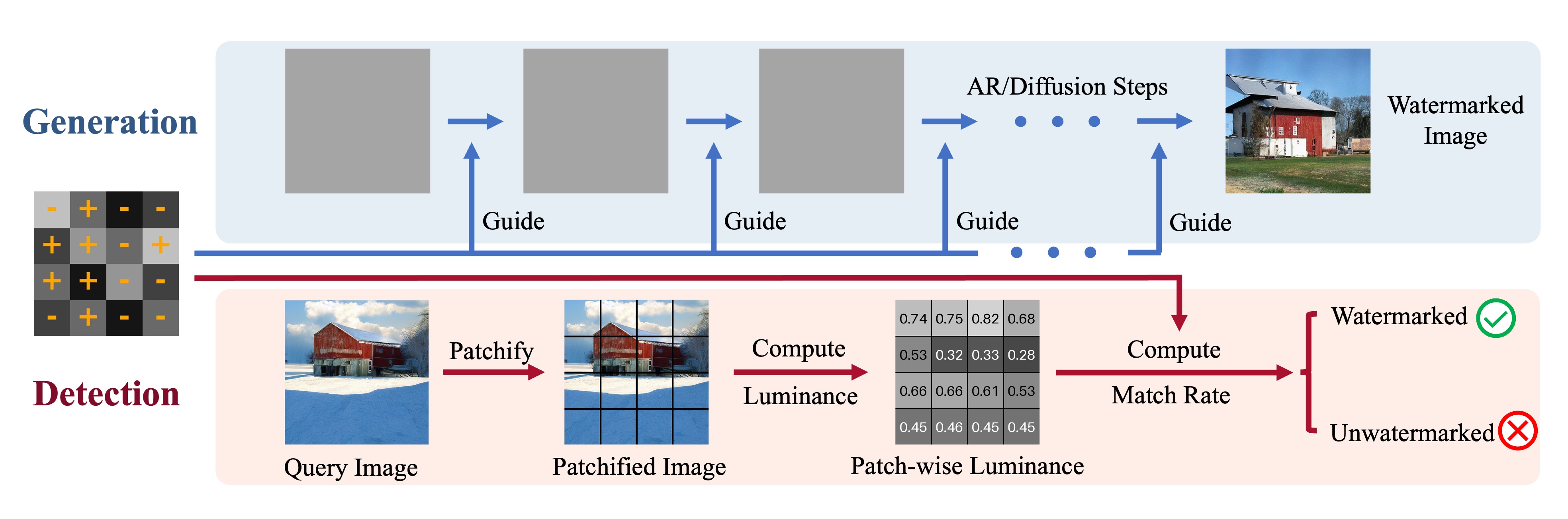
1. **New Watermark Mechanism**: Luminark partitions images into patches and computes their luminance values to create a binary pattern based on whether the luminance exceeds certain thresholds. This is akin to distinguishing areas with light from those without in a dark room.-
Training-Free, Plug-and-Play Operation: Luminark operates efficiently across various generative models without requiring additional training, much like how standard fuel works in different types of vehicles.
-
Strong Statistical Detection Guarantee: Luminark remains robust against image transformations and provides the statistical reliability needed for watermark detection. This is similar to safety equipment on an airplane that ensures reliable performance under diverse conditions.
📄 Full Paper Content (ArXiv Source)
Watermarking has long served as a key technique for protecting digital content in computer vision. With the rise of AI-generated media, its importance has increased substantially, driven by the increasing risks of misuse and unauthorized redistribution. However, designing a general-purpose watermarking method for vision generative models remains a significant challenge. The main difficulty arises from the diversity of modern generative modeling paradigms in computer vision——ranging from diffusion-based frameworks to autoregressive(AR) models ——each of which follows distinct design principles, neural network architectures, training objectives, and inference procedures.
Classical approaches embed signatures into the images’ frequency coefficients . Although broadly applicable, these methods suffer from limited robustness against common image transformations. Recently, a line of works has explored neural-network-based approaches, which either fine-tune the generative model’s parameters to synthesize watermarked output or train separate neural networks for watermark injection and detection . With careful data augmentation, these methods can achieve substantial robustness and maintain high perceptual quality. However, the black-box nature of neural networks provides no theoretical guarantees on detection reliability——users cannot rigorously evaluate when or why detection might fail, nor estimate the likelihood of such failures. Another line of work has proposed probabilistically-certified approaches that offer formal statistical guarantees for detection . Nevertheless, these methods are typically tailored to a specific generative paradigm and, according to our experiments, introduce degradation in image quality.
In this paper, we introduce Luminark, a new path to probabilistically-certified watermarking that (i) offers a strong statistical guarantee for detection, (ii) substantially outperform prior probabilistically-certified methods on the generation quality, (iii) remains robust against a variety of image transformations, and (iv) achieves this in a training-free, plug-and-play manner applicable to diverse generative paradigms.
Our first contribution is the introduction of a novel watermark for image protection. Given an image, we partition it into patches and compute the luminance value of each patch. The watermark is defined as a binary pattern over these luminance values—-whether each patch’s luminance exceeds a specified threshold. We mathematically show that if the binary pattern and thresholds are randomly chosen, the probability that an unwatermarked image (e.g., a natural image) matches the pattern decreases exponentially with respect to the number of patches, thereby making reliable detection feasible (supporting (i)). Moreover, since detection relies solely on patch-level statistics, it remains robust against common image transformations (supporting (iii)), such as smoothing, quantization, and compression.
From the service provider’s perspective, although detection in Luminark is straightforward, injecting the predefined pattern and maintaining high-quality generation is considerably more challenging. The second contribution of our work is the design of a training-free injection algorithm that enables Luminark to operate across diverse generative paradigms and generate visually convincing outputs. The key insight is that all recent generative paradigms, despite their differences, share a common mechanism—-the guidance technique . Guidance has become a standard tool in both diffusion and autoregressive vision models, where it enhances output quality by steering the generation process toward desired outcomes. We leverage this mechanism as the entry point for watermark injection (supporting (iv)) and introduce the watermark guidance, which directs each generation step toward alignment with the predefined pattern. This enables the watermark to be softly injected into the generation process in a plug-and-play manner, while simultaneously adjusting the content smoothly to preserve the quality of the generated image.
We conduct extensive experiments to evaluate the effectiveness of Luminark. Specifically, we test Luminark on diffusion models, autoregressive models, and hybrid solutions, including EDM2 , Stable Diffusion , VAR , and MAR , spanning model scales from a few hundred million to several billion parameters, covering diverse neural architectures (continuous and discrete tokenizers, U-Nets and Transformers), different output resolutions (256$`\times`$256, 512$`\times`$512 and 768$`\times`$768) and applications (vanilla class-conditional image generation and text-to-image generation). Experimental results demonstrate that Luminark largely outperforms previous probabilistically-certified baselines and preserves perceptual quality (supporting (ii)), while simultaneously achieving high detection rates against common image transformations. These results establish Luminark as a practical and general-purpose watermarking algorithm for vision generative models.
Related Works
Existing watermarking approaches in vision can be broadly classified into three distinct lines: classical post-hoc watermarking, neural-network-based watermarking, and probabilistically-certified watermarking.
Classical post-hoc watermarking refers to early approaches that inject a watermark into an image post hoc. To ensure imperceptibility, these methods typically transform the image into the frequency domain and adjust specific frequency coefficients to encode a signature . However, these approaches face a crucial trade-off between maintaining image quality and achieving robustness. Modifying low-frequency coefficients often leads to noticeable degradation in image quality, whereas modifying high-frequency coefficients makes the detection vulnerable to local perturbations . Owing to its efficiency and model-agnostic nature, this approach remains widely used, including in systems such as Stable Diffusion .
Neural-network-based watermarking. These approaches typically involve training a neural network to determine whether a query image contains a watermark. Regarding watermark injection, existing strategies generally follow three paradigms: some methods fine-tune the generative model itself, enabling it to synthesize watermarked content directly ; some methods utilize multiple techniques to fuse the watermark during generation without modifying the model parameters , such as training a plug-and-play “adapter” ; while others train a separate neural network as a post-hoc watermark injector . With careful data augmentations, these methods can achieve strong perceptual quality while maintaining detection robustness under common image distortions. However, owing to the inherent black-box nature of these models, users cannot rigorously evaluate when or why detection might fail, nor assess the reliability of a given detection outcome.
Probabilistically-certified watermarking injects a chosen random perturbation into the generative process so that the resulting distribution of outputs carries a statistically testable signal. Detection is then cast as a hypothesis test, checking whether a sample originates from the perturbed (watermarked) distribution rather than the original one. The test itself is typically tailored to the generative paradigm: diffusion models permit testing for structured patterns in the recovered noise, while autoregressive models test for distributional shifts in token statistics. As a result, different architectures require different perturbations and, consequently, different statistical tests. The pioneering work in this domain is the Tree-Ring watermark , which embeds a pattern into the initial noise vector of diffusion models. Detection is performed by inverting the generation process (via inverse ODE solvers) to recover the noise and verifying its alignment with the embedded pattern. Subsequent works have refined this concept with advanced designs . Recently, probabilistically-certified methods have also been proposed for autoregressive models , but these methods remain tightly coupled to specific generative paradigms. This architecture dependency limits their universality, and their visual fidelity remains considerably lower than neural-network-based watermarking approaches.
Watermarking as Luminance Constraints
Watermark Definition
In this work, we explore a novel watermarking mechanism for general image generation based on patch-level luminance statistics. In computer vision, luminance refers to the perceived brightness of a pixel, derived from its RGB values . It represents the grayscale intensity that a human observer would perceive from a colored image.
Mathematically, we first partition an image $`\mathbf{x}`$ of size $`H\times W`$ into non-overlapping patches of size $`k\times k`$, i.e., $`\mathbf{x}=\{\mathbf{p}_1, \mathbf{p}_2,\dots, \mathbf{p}_N\}`$, where $`\mathbf{p}_1`$ denotes the patch in the top-left corner and $`\mathbf{p}_N`$ corresponds to the patch in the bottom-right corner. The total number of patches $`N`$ is given by $`\frac{H\times W}{k^2}`$. For each patch $`\mathbf{p}_i`$, we compute the average pixel values (normalized into $`(0,1)`$ in the R, G, and B channels, denoted as $`(\overline{R}_i,\overline{G}_i,\overline{B}_i)`$. The luminance of the patch is then defined as:
\begin{equation}
l(\mathbf{p}_i) = 0.299\cdot\overline{R}_i + 0.587\cdot\overline{G}_i + 0.114\cdot\overline{B}_i.
\label{eq:luminance}
\end{equation}We denote the luminance of $`\mathbf{x}`$ as vector $`\mathbf{L}(\mathbf{x})=(l(\mathbf{p}_1), l(\mathbf{p}_2), \dots, l(\mathbf{p}_N))`$. To avoid confusion, we denote the generated and real images as $`\mathbf{x}_{\text{gen}}`$ and $`\mathbf{x}_{\text{real}}`$, respectively. Our goal is to inject specific patterns (i.e., signature) into the generation process of $`\mathbf{x}_{\text{gen}}`$ such that its luminance $`\mathbf{L}(\mathbf{x}_{\text{gen}})`$ becomes statistically distinguishable from that of the real image $`\mathbf{x}_{\text{real}}`$, thereby enabling watermark detection. To construct this statistical difference, we first define a binary pattern $`\mathbf{c}=(c_1,c_2,\dots,c_N)\in \{-1,1\}^N`$ and a real-valued threshold vector $`\boldsymbol{\tau}=(\tau_1, \tau_2,\dots,\tau_N)\in (0,1)^N`$. Both values in $`\mathbf{c}`$ and $`\boldsymbol{\tau}`$ can be randomly generated using a pseudo-random number generator, fixed by the service provider, and are not released to the web users.
The real-valued vector $`\boldsymbol{\tau}`$ is used to access the “level” of luminance. For each patch $`i`$, we compute a decision stump of the form $`\operatorname{sgn}[l(\mathbf{p}_i)-\tau_i]`$, which evaluates whether the patch’s luminance exceeds $`\tau_i`$. The sign function $`\operatorname{sgn}(.)`$ returns the sign of a real number, outputting $`-1`$ for negative inputs, and $`+1`$ for non-negative inputs. Applying this across all patches yields the binary pattern of $`\mathbf{x}`$:
\begin{equation*}
\mathbf{o}(\mathbf{x})=(\operatorname{sgn}[l(\mathbf{p}_1)-\tau_1],\cdots,\operatorname{sgn}[l(\mathbf{p}_N)-\tau_N])\in \{-1,1\}^N.
\end{equation*}Detection is performed by comparing the similarity of the binary pattern of the image $`\mathbf{o}(\mathbf{x})`$ and the predefined $`\mathbf{c}`$. Intuitively, if both $`\mathbf{c}`$ and $`\boldsymbol{\tau}`$ are randomly selected and known only to the provider, a natural image is unlikely to match the pattern by chance. Therefore, if the image pattern $`\mathbf{o}(\mathbf{x})`$ sufficiently differs from $`\mathbf{c}`$, the image $`\mathbf{x}`$ is identified to be unwatermarked. A statistical analysis and a more rigorous detection algorithm are presented in Section 3.2.
For completeness, we denote a watermark $`\mathcal{W}=(\mathbf{c}, \boldsymbol{\tau})`$. This approach offers several key advantages. First and most notably, the watermark is designed to be imperceptible to humans, as it operates on the average luminance of each patch rather than injecting pixel-level patterns. Furthermore, the use of patch-level average luminance as the signature provides inherent robustness against several popularly studied image manipulations. The averaging calculation acts as a low-pass filter, making the signature resilient to random perturbations like added noise or artifacts from mild compression. Such modifications are unlikely to alter the average luminance of a patch enough to flip its outcome relative to the threshold, thus preserving the integrity of the watermark.
Probabilistically-Certified Watermark Detection
The objective of watermark detection is to reliably determine whether a given query image $`\mathbf{x}`$ has been injected with a specific predefined watermark. We begin by defining the core metric for our test. For a given image $`\mathbf{x}`$ and watermark $`\mathcal{W}=(\mathbf{c}, \boldsymbol{\tau})`$, recall that $`\mathbf{x}`$ is partitioned into $`N`$ patches $`\{\mathbf{p}_i\}_{i=1}^N`$. We define the match rate, $`m(\mathbf{x}, \mathcal{W})`$, as fraction of patches whose luminance statistics align with the watermark’s binary pattern $`\mathbf{c}`$:
\begin{equation}
    m(\mathbf{x}, \mathcal{W})=\frac1N\sum_{i=1}^N\mathbb{I}[\operatorname{sgn}(l(\mathbf{p}_i)-\tau_i)=c_i]
\end{equation}where $`\mathbb{I}[\cdot]`$ is the indicator function.
We next show that, for an unwatermarked (e.g., natural) image, its match rate can be well controlled with high probability if $`\mathcal{W}`$ is randomly chosen.
Proposition 1. *Assume each $`c_i`$ is drawn i.i.d from $`\operatorname{Bernoulli}(\frac{1}{2})`$ with support $`\{-1,1\}`$ and each $`\tau_i`$ is drawn i.i.d from any distribution with support $`(0,1)`$, then for any fixed $`\mathbf{x}`$, for any $`0 \leq \varepsilon \leq \frac{1}{2}`$, we have
\begin{align}
        \Pr(m(\mathbf{x}, \mathcal{W})\geq \frac{1}{2} + \varepsilon) &=\frac{1}{2^N}\sum\limits_{k=\lceil N(\frac{1}{2}+\varepsilon)\rceil}^{N}\binom{N}{k} \\
        &\leq \exp(-N\cdot D_{KL}(\varepsilon))
\end{align}where $`D_{KL}(\varepsilon)=(\frac{1}{2}+\varepsilon)\ln(1+2\varepsilon)+(\frac{1}{2}-\varepsilon)\ln(1-2\varepsilon)`$ and $`\lceil y \rceil`$ denotes the smallest integer that is no less than $`y`$.*
Proposition 1 shows that the probability of an unwatermarked image achieving a match rate substantially exceeding $`\frac{1}{2}`$ decreases exponentially with the number of patches $`N`$. Hence, one can set the detection threshold slightly above $`\frac{1}{2}`$, and the false positive rate, i.e., the probability of misclassifying an unwatermarked image as a watermarked one, can be controlled with statistical guarantees. The proof is provided in Appendix 6.
In practice, for the detection threshold, since $`m(\mathbf{x}, \mathcal{W})`$ follows a binomial distribution $`B(N, \frac{1}{2})`$, we can directly compute the threshold $`T_{match}`$ for a target false positive rate $`fpr`$ (e.g. $`1\%`$). Specifically, each candidate threshold $`\frac{k}{N}`$ has an associated p-value, which is the probability that a natural image achieves a match rate of at least $`\frac{k}{N}`$ under the binomial distribution. To find the threshold corresponding to the desired $`fpr`$, we iterate through candidate thresholds from $`k=0`$ to $`k=N`$, compute the corresponding p-value for each, and select the first threshold whose associated p-value is at most $`fpr`$. The full procedure is summarized in Algorithm [alg:set_threshold_final]. With a properly calibrated $`T_{match}`$, the final detection process for a query image $`\mathbf{x}`$ becomes straightforward. As described in Algorithm [alg:detection_final], we first compute its match rate $`m(\mathbf{x}, \mathcal{W})`$. If this value exceeds $`T_{match}`$, the image is classified as watermarked; otherwise, it is deemed unwatermarked.
$`p_k \gets \frac{1}{2^N} \sum_{i=k}^N \binom{N}{i}`$ $`T_{match} \gets k/N`$ break $`T_{match}`$
Let $`\{\mathbf{p}_1, \dots, \mathbf{p}_N\}`$ be the patches of $`\mathbf{x}`$. $`m \gets \frac1N\sum_{i=1}^{N} \mathbb{I}\left[ \operatorname{sgn}(l(\mathbf{p}_i) - \tau_i) = c_i \right]`$ return $`(m\ge T_{match})`$
Watermark Injection via Step-wise Guidance
Originally proposed in the diffusion model literature, guidance has since become widely adopted in vision generation. For context, consider a diffusion model $`D(\mathbf{x}_t, \sigma_t)`$ trained to progressively denoise a noisy input $`\mathbf{x}_t`$ at time $`t`$. The sampling process is then a deterministic step-by-step denoising procedure that transforms Gaussian noise into a clean image, which can often be described by an ordinary differential equation (ODE) : $`\frac{\mathrm{d}\mathbf{x}_t}{\mathrm{d}t}=\frac{\mathbf{x}_t-D(\mathbf{x}_t,\sigma_t)}{\sigma_t}`$, $`\quad \mathbf{x}_T\sim\mathcal{N}(0,\sigma_{\text{max}}^2\mathbf{I})`$, where $`\sigma_{\text{max}}`$ is the initial noise level at the start of the sampling process. In practice, this continuous process is approximated by numerical solvers such as the Euler method or Runge-Kutta methods . Using the Euler method as an illustration, the generation process can be written as
\begin{align}
    \mathbf{x}_{t-1}=\mathbf{x}_t-\underbrace{\frac{{\mathbf{x}}_t-D({\mathbf{x}}_t,\sigma_t)}{\sigma_t}}_{\text{Denoising Term}}(\sigma_t-\sigma_{t-1}),\quad t=T,\dots,1
\end{align}Guidance techniques introduce additional modifications into Eqn.(4) to improve the quality of the generated images at each sampling step. For example, Classifier Guidance(CG) modifies the update direction using an image classifier $`p(y|\mathbf{x}_t)`$:
\begin{equation}
\begin{split}
    &\mathbf{x}^{\texttt{CG}}_{t-1}=\mathbf{x}^{\texttt{CG}}_t-\bigg[
    \underbrace{\frac{\mathbf{x}^{\texttt{CG}}_t-D(\mathbf{x}^{\texttt{CG}}_t,\sigma_t)}{\sigma_t}}_{\text{Denoising Term}}+ \\ &\underbrace{s_t\nabla_{\mathbf{x}^{\texttt{CG}}_t} \log p(y|\mathbf{x}^{\texttt{CG}}_t;\sigma_t}_{\text{Classifier Guidance Term}})\bigg](\sigma_t-\sigma_{t-1}),\quad t=T,\dots,1
\end{split}
\end{equation}where $`s_t`$ is a scale parameter that depends on the time $`t`$. Shortly thereafter, researchers generalized the concept of guidance beyond classifier-based targets. Notable extensions include Classifier-Free Guidance and Auto-Guidance . More recently, guidance has also been directly applied to other iterative generative frameworks, including autoregressive models and autoregressive-diffusion hybrid models , yielding significant performance gains.
We believe that guidance is well-suited to our scenario for two main reasons. First, prior studies have shown that guidance can be effectively applied across diverse generative paradigms, thereby satisfying the requirement for a general-purpose watermarking mechanism. Second, its inherent training-free nature makes guidance especially suitable for watermark injection: by defining a metric that quantifies the discrepancy between an intermediate generated image and the target watermark $`\mathcal{W}`$, the guidance process can progressively adjust the outcome in an adaptive manner.
Inspired by these works, we develop the Watermark Guidance(WG) to softly enforce the luminance constraints $`\mathcal{W}`$ during generation. We first define an almost everywhere differentiable penalty function $`\text{{Penalty}}(\mathbf{x}, \mathcal{W})`$, serving as a surrogate of the match rate $`m(\mathbf{x}, \mathcal{W})`$ using a hinge-like loss:
\begin{equation}
\text{{Penalty}}(\mathbf{x}, \mathcal{W}) = \sum_{i=1}^{N} \max\{0, c_i\cdot(\tau_i-l(\mathbf{p}_i))\}.
\label{eq:violation_loss}
\end{equation}The inner term $`c_i\cdot(\tau_i-l(\mathbf{p}_i))`$ is positive if and only if the constraint for patch $`i`$ is violated, and the $`\max\{0,\cdot\}`$ operation ensures that satisfying all constraints contributes zero loss. We replace the original guidance term in Eqn.(5) with this penalty and obtain the watermark-guided update:
\begin{equation}
\begin{split}
    &\mathbf{x}^{\texttt{WG}}_{t-1}=\mathbf{x}^{\texttt{WG}}_t-\left[\underbrace{\frac{\mathbf{x}^{\texttt{WG}}_t-D(\mathbf{x}^{\texttt{WG}}_t,\sigma_t)}{\sigma_t}}_{\text{Denoising Term}}\right.\\
&\left.+\underbrace{s_t\nabla_{\mathbf{x}^{\texttt{WG}}_t}\text{{Penalty}}( \mathbf{x}^{\texttt{WG}}_{t}, \mathcal{W}) }_{\text{Watermark Guidance Term}}\right](\sigma_t-\sigma_{t-1}),\quad t=T,\dots,1
\end{split}
\end{equation}The full procedure is outlined in Algorithm [alg:pixel_guided_sampler]. Above, we demonstrated our watermark guidance mechanism in the context of pixel-level diffusion models using the Euler method. One potential concern is the difficulty of extending our method to more complex settings. However, it is worth noting that in most recent models, guidance is typically formulated as additive terms within the step-wise update. To integrate our approach, we can simply either (a) apply watermark guidance to these models by replacing existing guidance terms, or (b) combine it with other additive guidance by simply appending the additional term. Appendix 9 and 10 provide detailed generation pipelines in representative models and the corresponding watermark injection implementations.
Input: Denoiser model $`D(\mathbf{x},\sigma)`$, diffusion steps $`T`$, noise schedule $`\{\sigma_t\}_{t=0}^T`$, watermark $`\mathcal{W}=(\mathbf{c}, \boldsymbol{\tau})`$, watermark guidance scale $`s`$, threshold $`T`$ Initialize: sample $`\mathbf{x}_T \sim \mathcal{N}(0, \sigma_T^2\mathbf{I})`$ $`\mathbf{x}_{t-1}\leftarrow\mathbf{x}_t-\Big[\underbrace{\frac{\mathbf{x}_t-D(\mathbf{x}_t,\sigma_t)}{\sigma_t}}_{\text{Denoising}}`$ $`+ \underbrace{s\nabla_{\mathbf{x}_t}\text{Penalty}( \mathbf{x}_{t}, \mathcal{W}) }_{\text{Guidance}}\Big](\sigma_t-\sigma_{t-1})`$
$`m \gets \sum_{i=1}^{N} \mathbb{I}\!\left[\operatorname{sgn}(l(\mathbf{p}_i)-\tau_i)=c_i\right]`$ return $`\mathbf{x}_0`$
Experiment
For a comprehensive comparison, we conduct experiments on nine state-of-the-art ImageNet-pretrained generative models, as summarized in Table [tab:model_description]. These models span diverse architectures, parameter scales, and configurations. Building on this foundation, we adopt ImageNet as our primary experimental platform. Due to space limitations, the detailed baseline descriptions, hyperparameters, visualization, and extended results on the text-to-image scenario are provided in the appendix.
Robustness
Robustness aims to assess whether a watermark remains detectable after image transformations introduced by potential adversaries. In this subsection, we examine the robustness of our method against a range of practical image manipulations and compare its performance with baseline approaches.
We compare Luminark against four certified methods: classical approaches DwtDct , DwtDctSvd , and modern watermarking approaches in Tree-Ring family: Gaussian-Shading (GS) and PRC-W . The DwtDct and DwtDctSvd baselines are evaluated across all models, whereas the latter two are diffusion-specific, so we evaluate them only on EDMs. For all baselines, we use the official implementation if provided 1. For our approach, the hyperparameters (e.g., patch size and watermark guidance scale) is provided in Appendix 12. For each experiment, we first draw a unique watermark for each method and keep it fixed. Then, for every method, we sample 1,000 unwatermarked and 1,000 watermarked images. To assess robustness, each image is further subjected to nine different transformations: Scaling, Cropping, JPEG Compression, Filtering, Smoothing, Color Jitter, Color Quantization, Gaussian Noise, and Sharpening. The implementation for each transformation is detailed in Appendix 7. We then re-apply watermark detection for each method on the transformed images and measure the detection accuracy. Each experiment is repeated 20 times with different random seeds to test the influence of watermark patterns and the sampled images. The average performance is reported.
| Model | Paradigm | Tokenizer | Resolution | Param. | ||||
|---|---|---|---|---|---|---|---|---|
| (lr-0.1em)6-9 | GS. | PRC-W. | Ours | Ref. | ||||
| EDM2-XS | Diffusion | Continuous | 512$`\times`$512 | 0.25 B | 3.53 | |||
| EDM2-L | Diffusion | Continuous | 512$`\times`$512 | 1.56 B | 2.06 | |||
| EDM2-XXL | Diffusion | Continuous | 512$`\times`$512 | 3.05 B | 1.81 | |||
| VAR-d16 | AR. | Discrete | 256$`\times`$256 | 0.31 B | 3.47 | |||
| VAR-d30 | AR. | Discrete | 256$`\times`$256 | 2.01 B | 2.05 | |||
| VAR-d36 | AR. | Discrete | 512$`\times`$512 | 2.35 B | 2.76 | |||
| MAR-Base | Hybrid | Continuous | 256$`\times`$256 | 0.21 B | 2.31 | |||
| MAR-Large | Hybrid | Continuous | 256$`\times`$256 | 0.48 B | 1.78 | |||
| MAR-Huge | Hybrid | Continuous | 256$`\times`$256 | 0.94 B | 1.55 |
Experimental Results. The experimental results are reported in Table [tab:robustness]. It can be seen that in all settings, our method consistently achieves accuracies of at least $`\geq`$95%, highlighting its wide applicability across different generative paradigms and reliable detectability under diverse transformations. Relative to prior methods, Luminark significantly outperforms post-hoc baselines (DwtDct $`\sim58\%`$, DwtDctSvd $`\sim65\%`$, RivaGAN $`\sim`$82%). Even when compared with diffusion-specific approaches on EDMs, Luminark remains highly competitive: its average performance is nearly the same as PRC-W and only marginally below Gaussian-Shading. We attribute the success of Luminark to its use of a regional statistical signature that is inherently more robust—while individual pixel values may vary, the patch-wise statistical properties are largely preserved. Due to space limitations, we cannot test all possible transformations. A natural concern is that certain common operations, such as flipping, could lead to huge detection mistakes. This issue can be addressed with a straightforward strategy: for any given image, we apply the watermark detector to both the original and its flipped version, and then use the logical “OR” of the two outcomes as the final detection result.
Fidelity
Following standard practice, we use the Fréchet Inception Distance (FID) to evaluate the generation quality of image generative models. We conduct experiments on the same set of models as in Section 4.1 and compare Luminark with Gaussian-Shading and PRC-W. The three post-hoc baselines are excluded from this evaluation due to their weak robustness. For each experiment, we first sample a unique watermark for each method and keep it fixed. Then, for each method, we generate 50,000 watermarked images and compute the FID scores against the clean image dataset. Each experiment is repeated 20 times, and the average performance is reported.
Experimental Results. As shown in Table [tab:model_description], the FID scores of watermarked images with Luminark significantly surpass those of Gaussian-Shading and PRC-W, while closely approaching the non-watermarked references across all nine models. The differences between Luminark and the reference values are generally around 1.0. Notably, the FID of watermarked EDM2-XXL is only 2.13, demonstrating exceptionally high generation quality. In comparison, Gaussian-Shading and PRC-W nearly double the reference FID score, not to mention they are not applicable in VAR and MAR. We further extend the evaluation to Stable Diffusion v2.1, using MS-COCO validation set (30K samples). The FID and CLIP score are reported in Table [tab:SD_fid].
r4.5cm
| Methods | FID $`\downarrow`$ | CLIP $`\uparrow`$ |
|---|---|---|
| Ref. | 26.83 | 0.3329 |
| GS. | 26.27 | 0.3302 |
| PRC-W. | 26.33 | 0.3314 |
| Ours | 26.00 | 0.3320 |
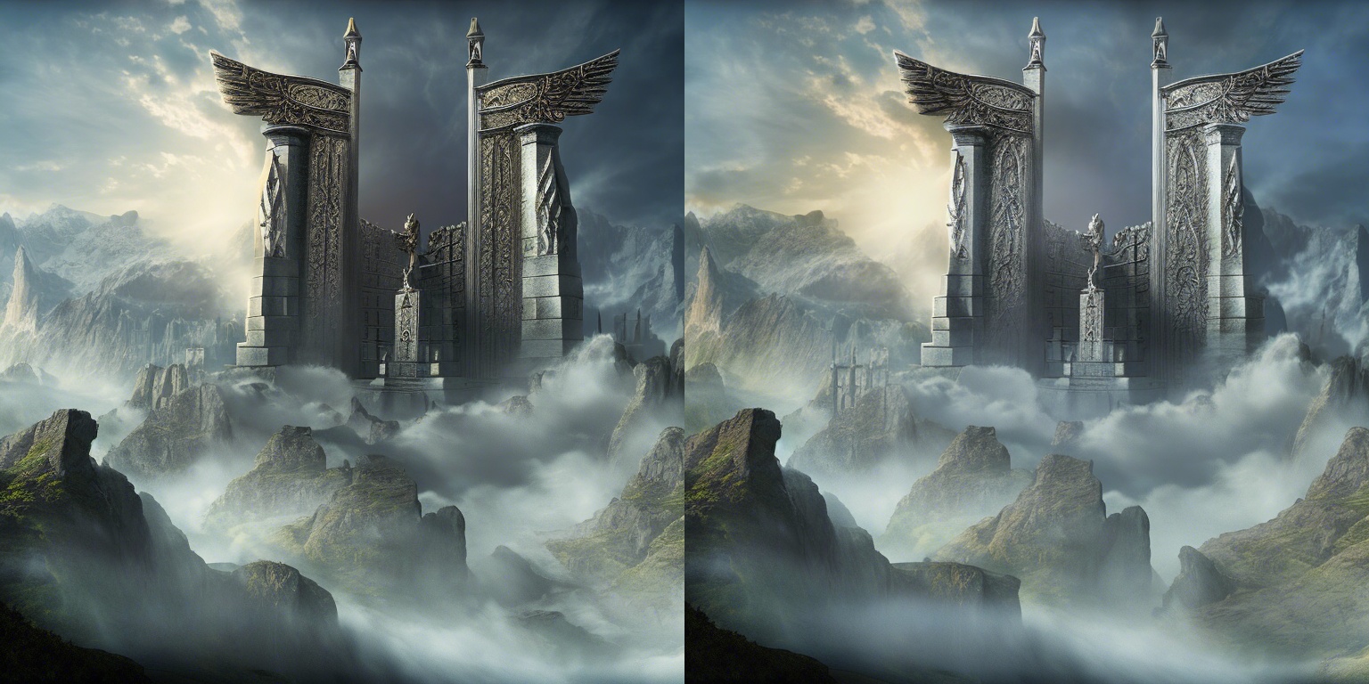
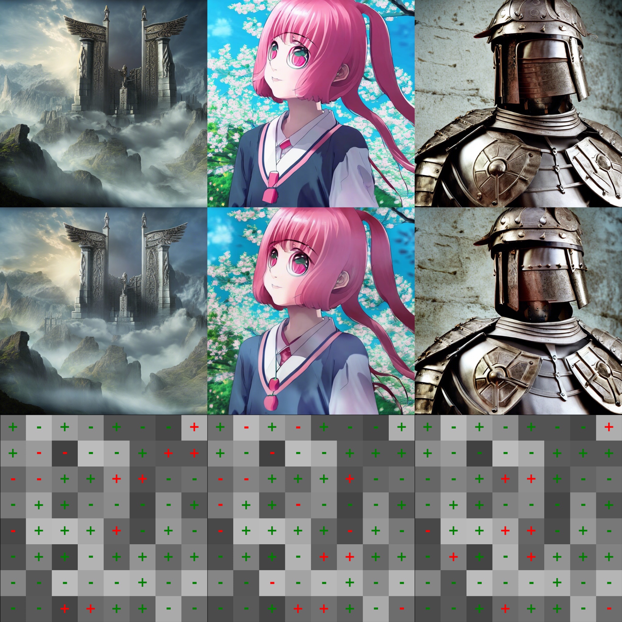
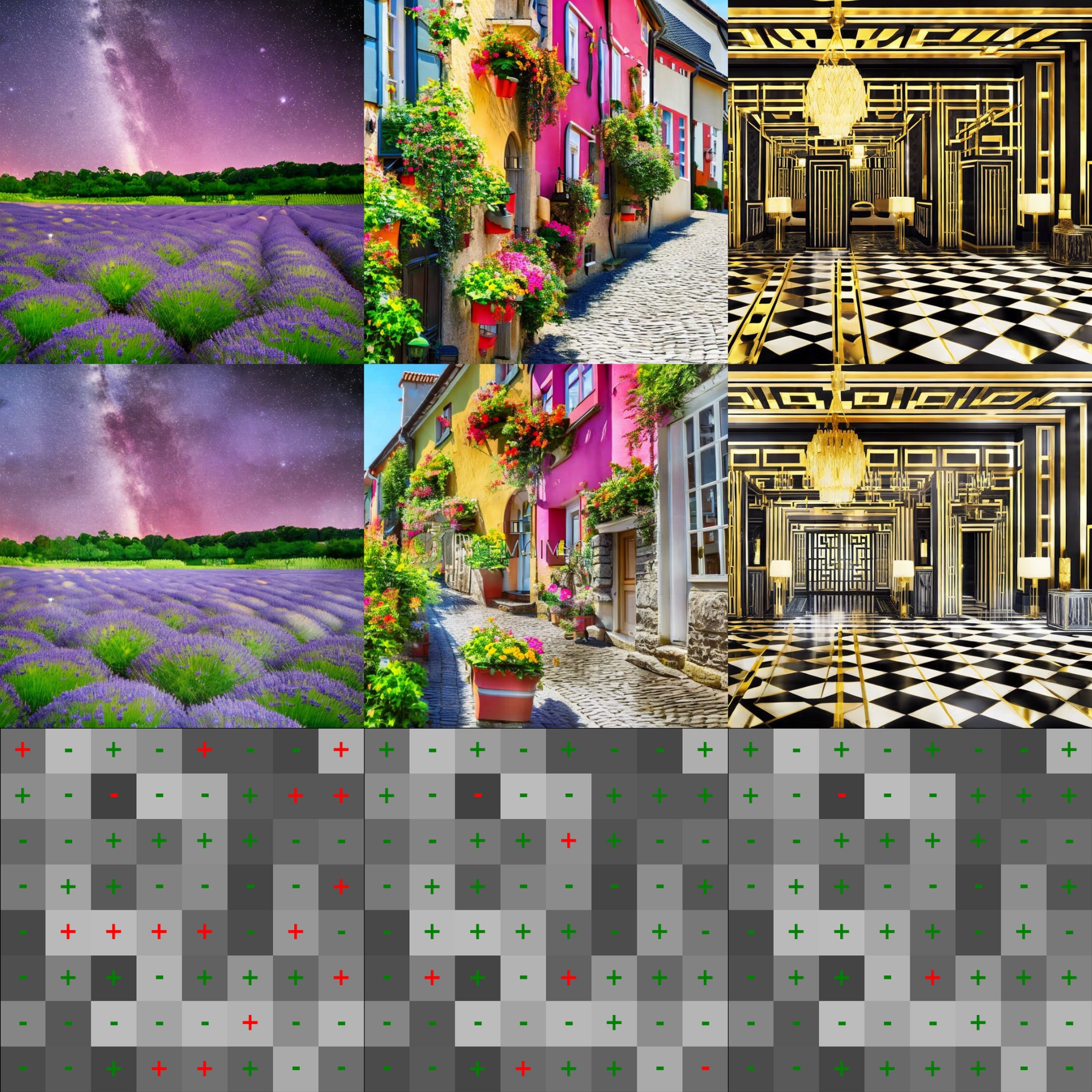
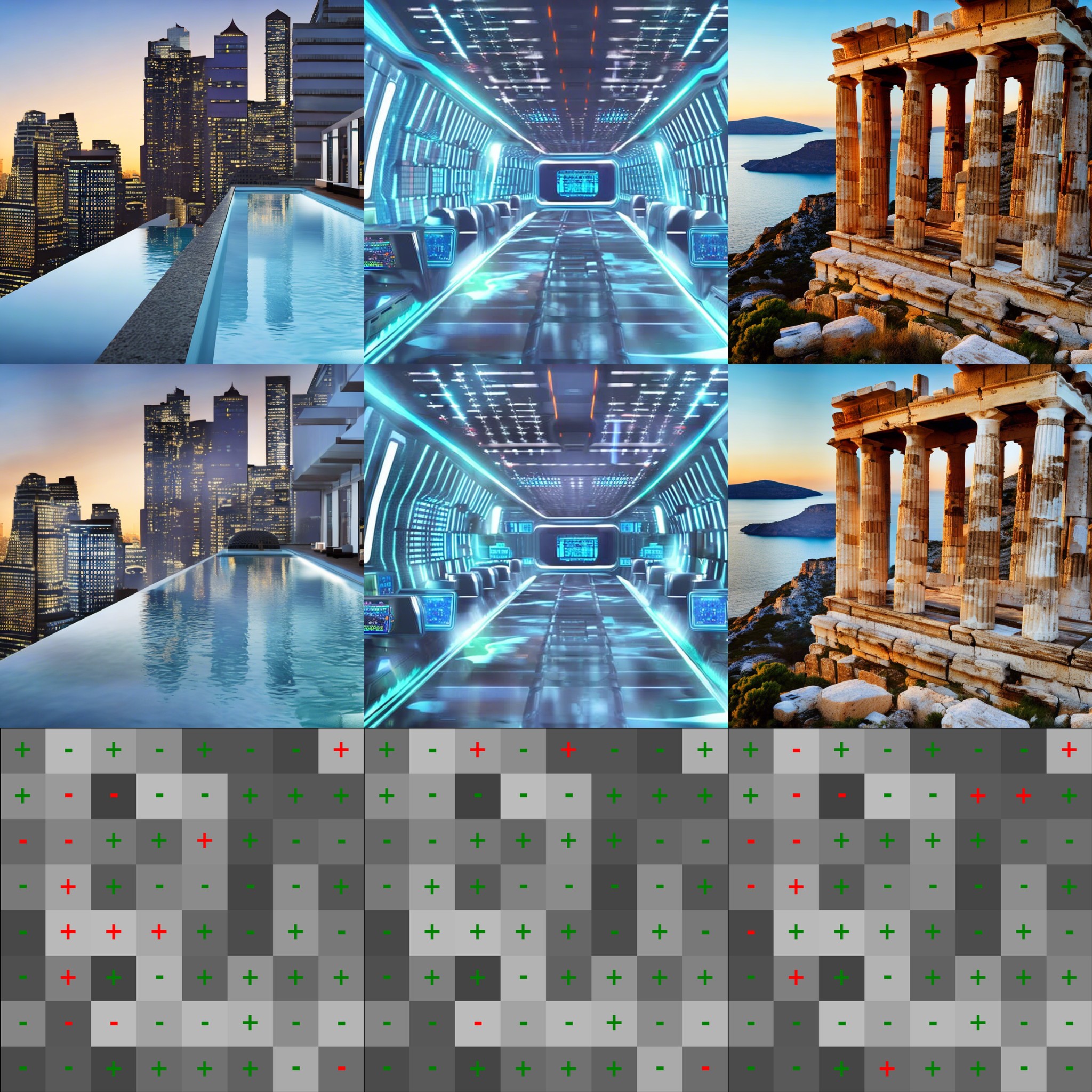
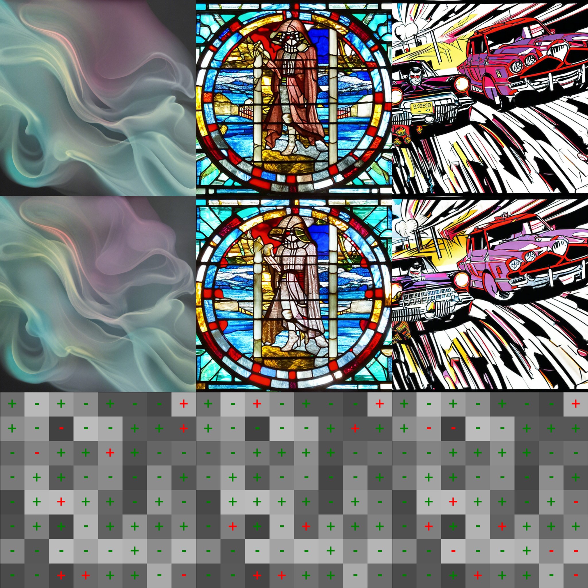
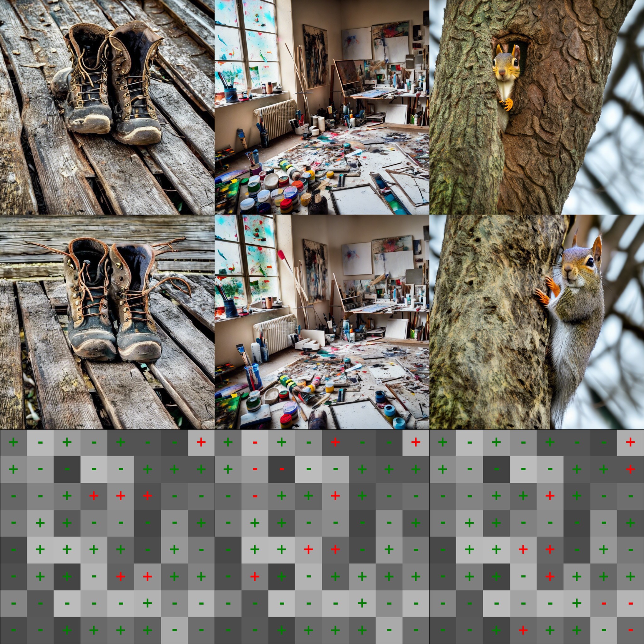
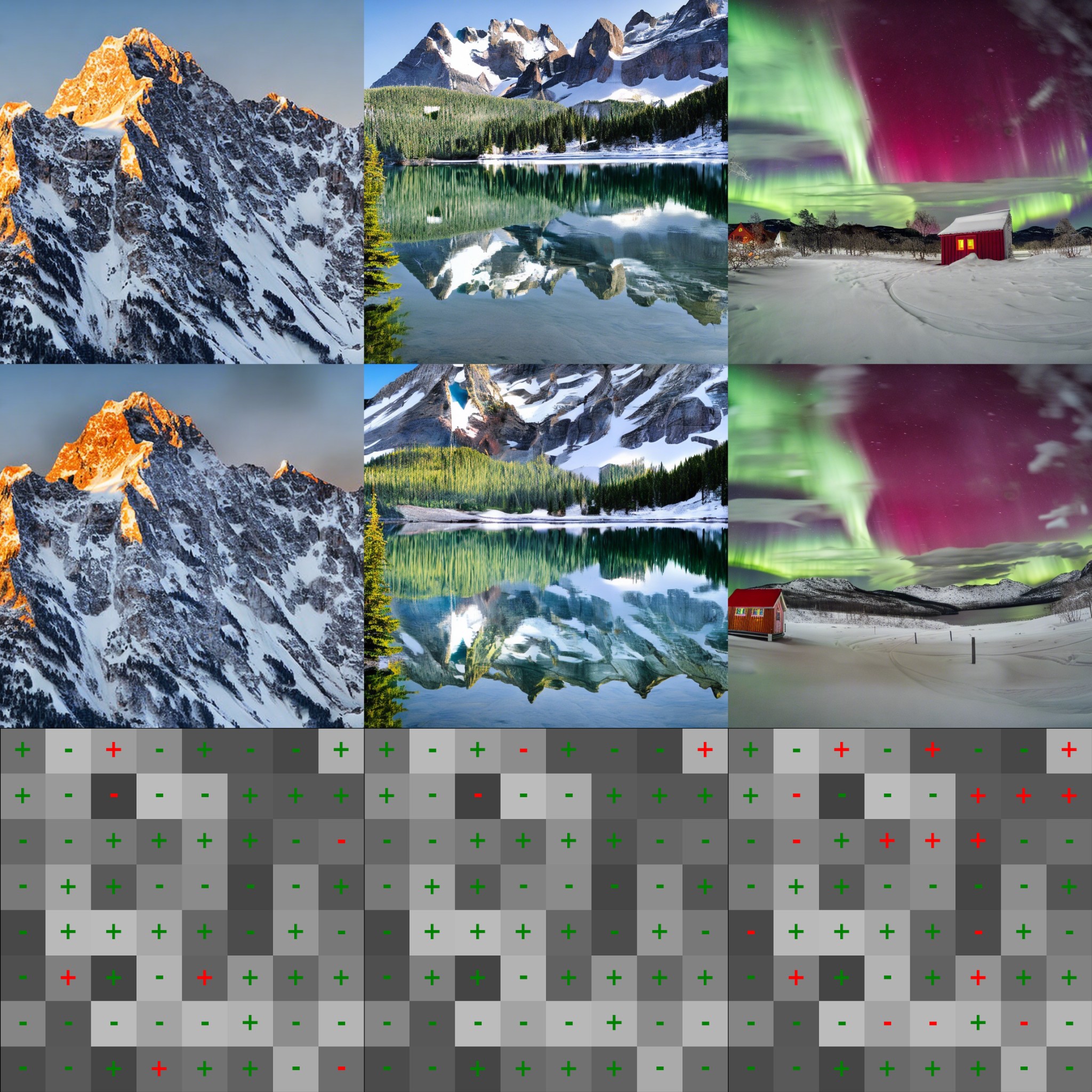
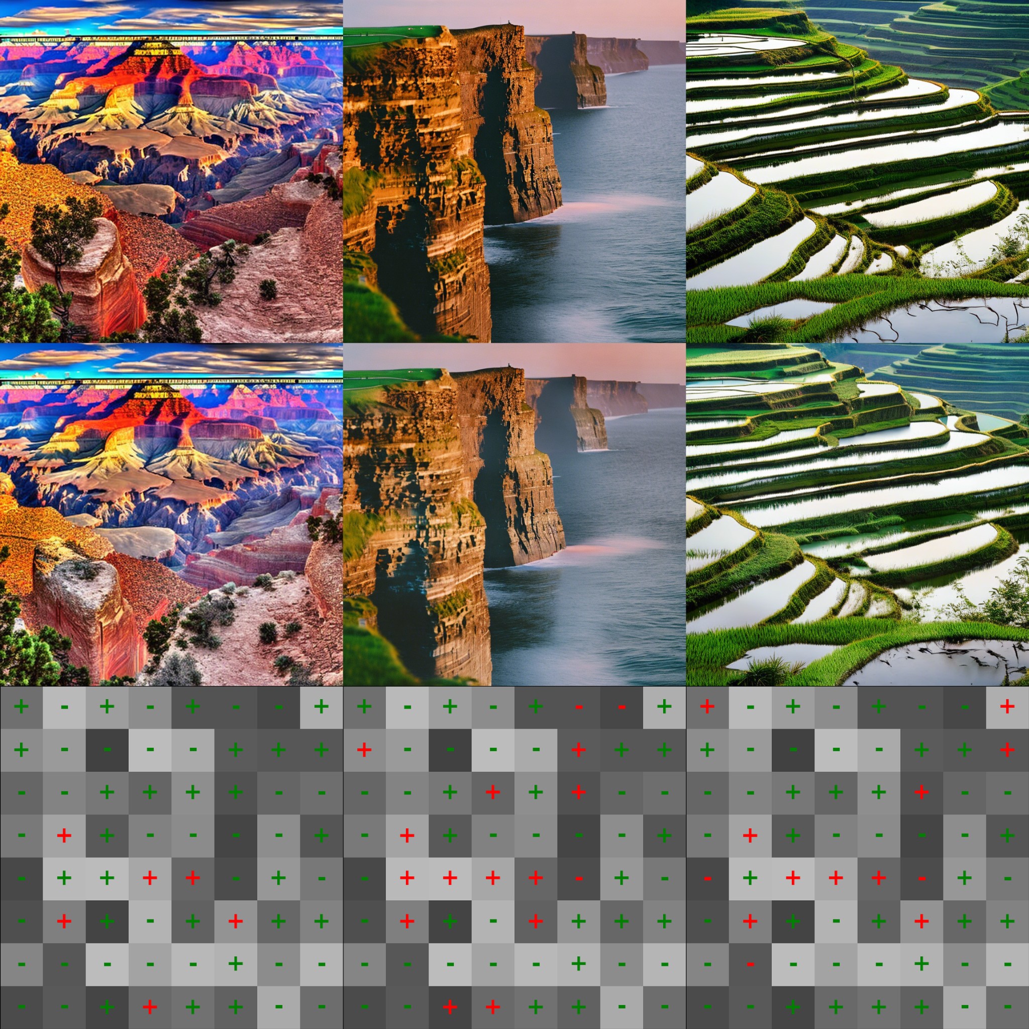
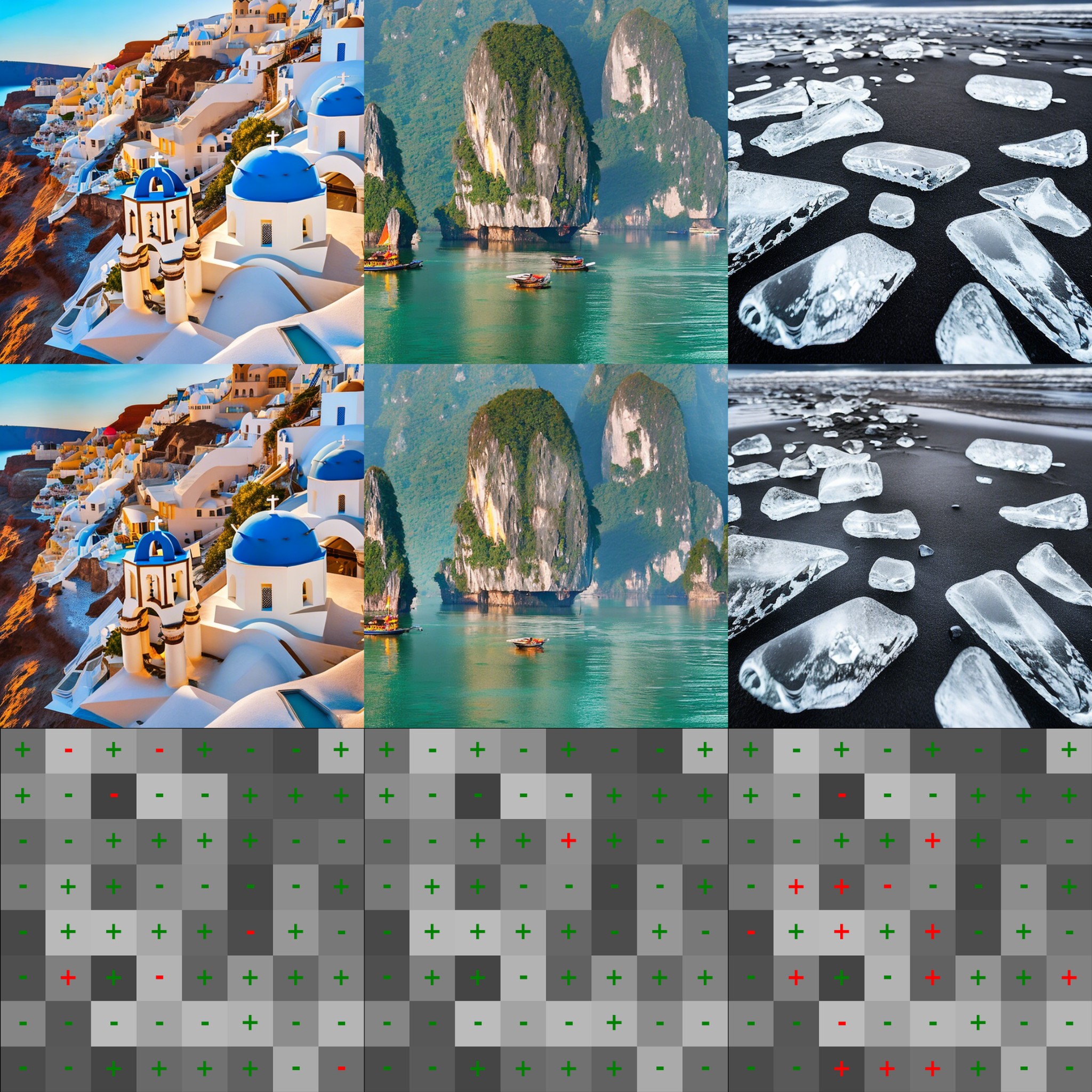
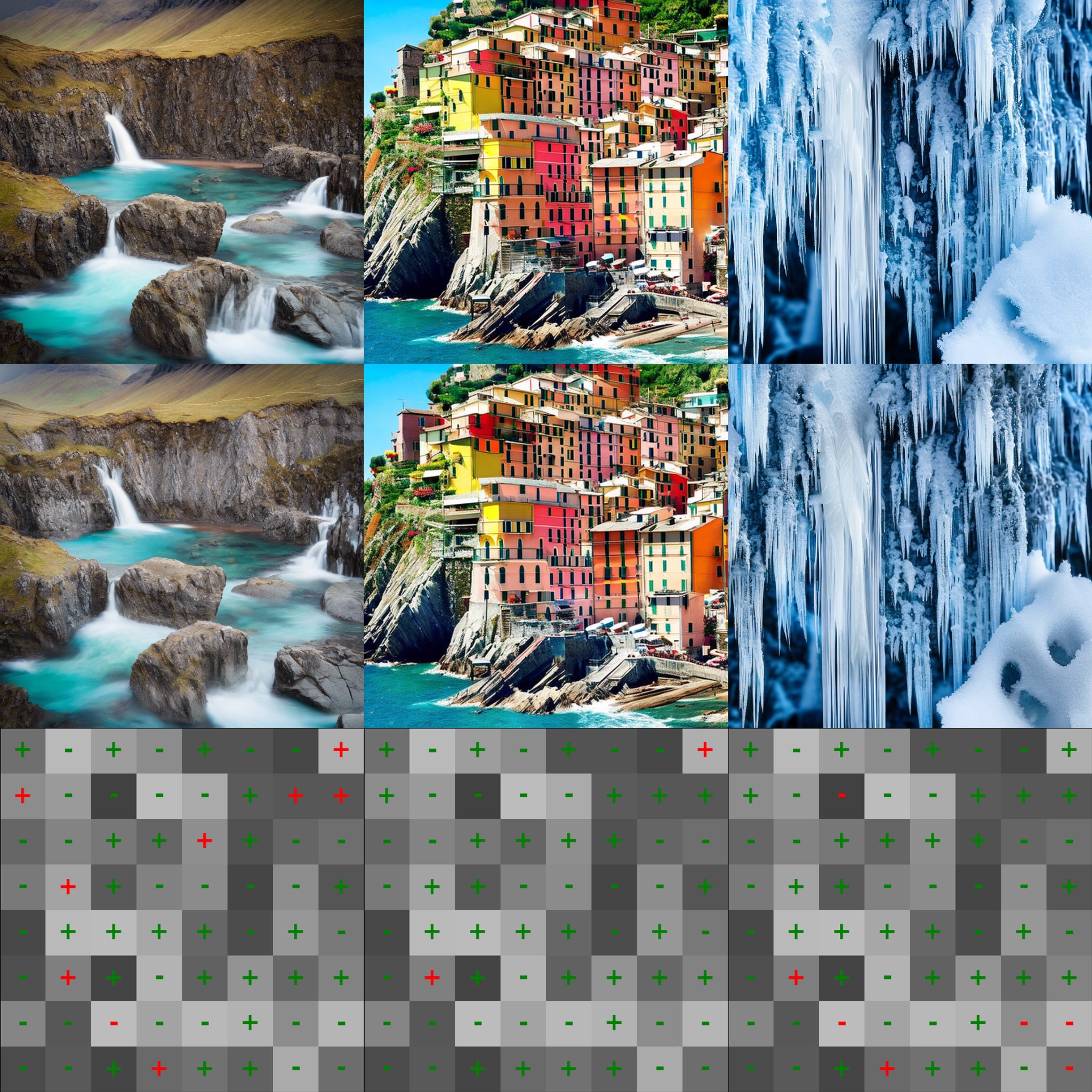
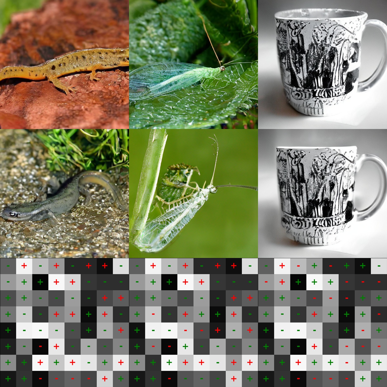
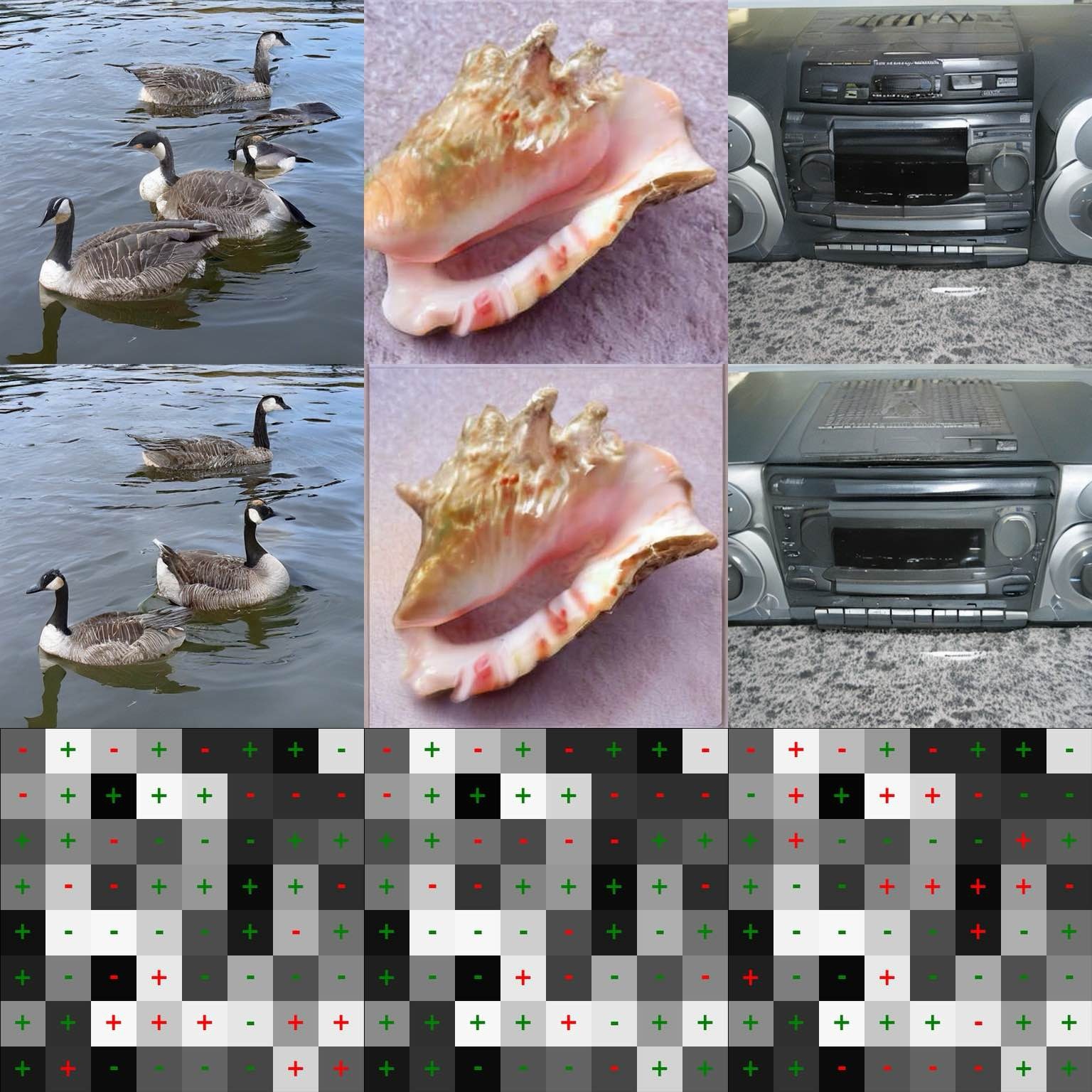
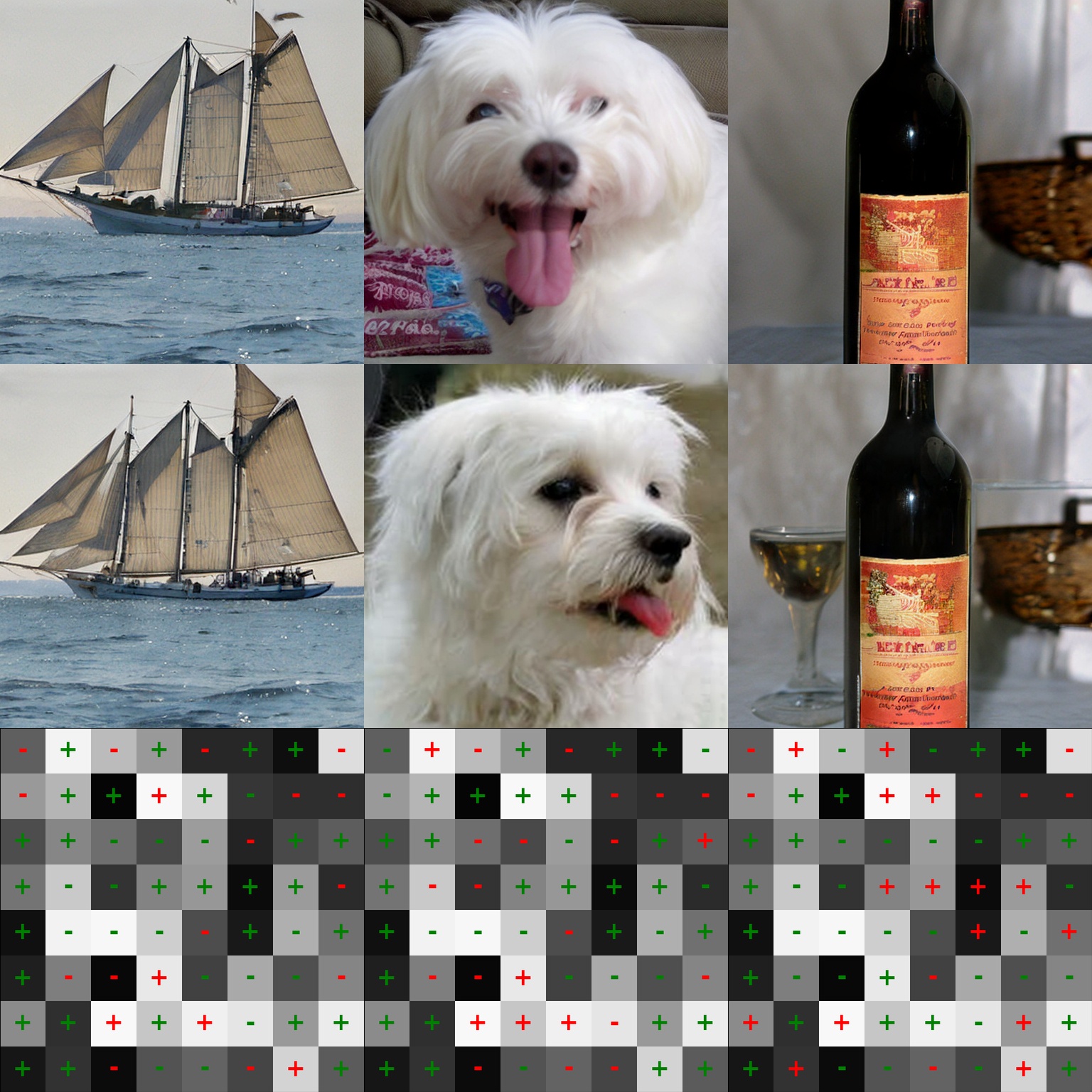
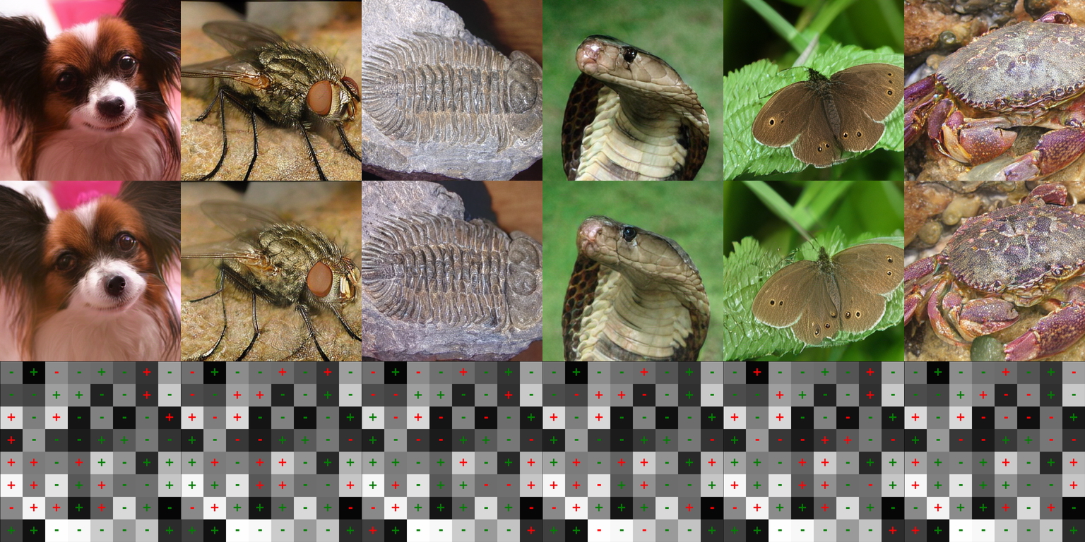
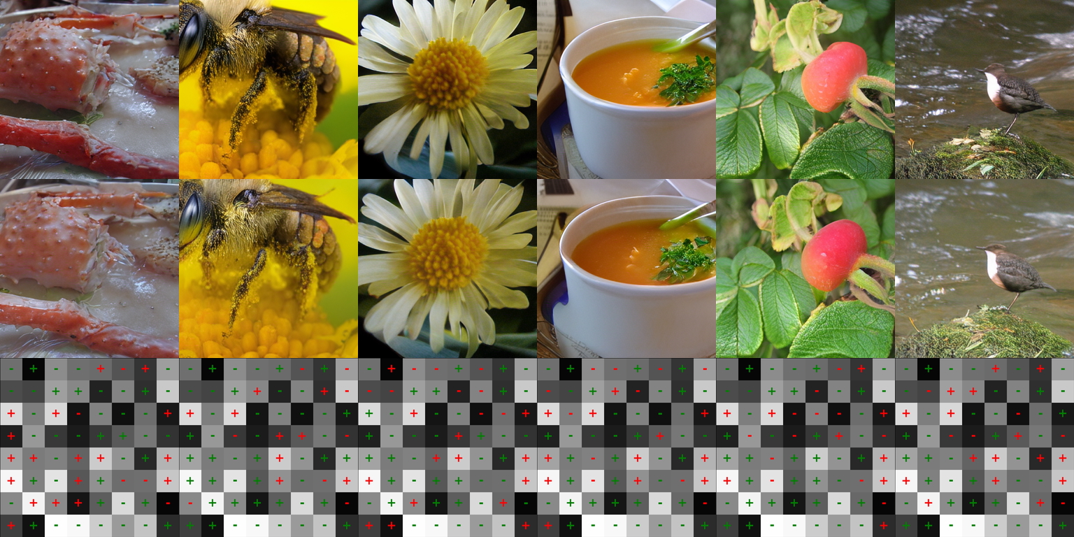
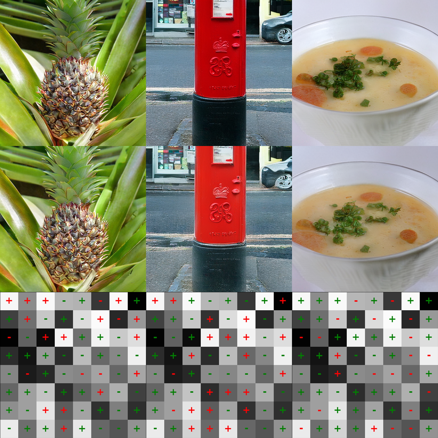
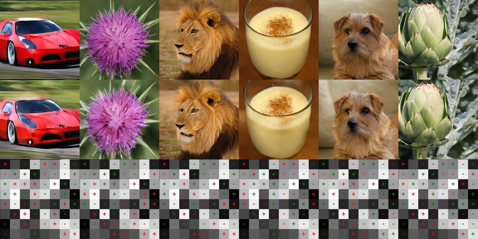
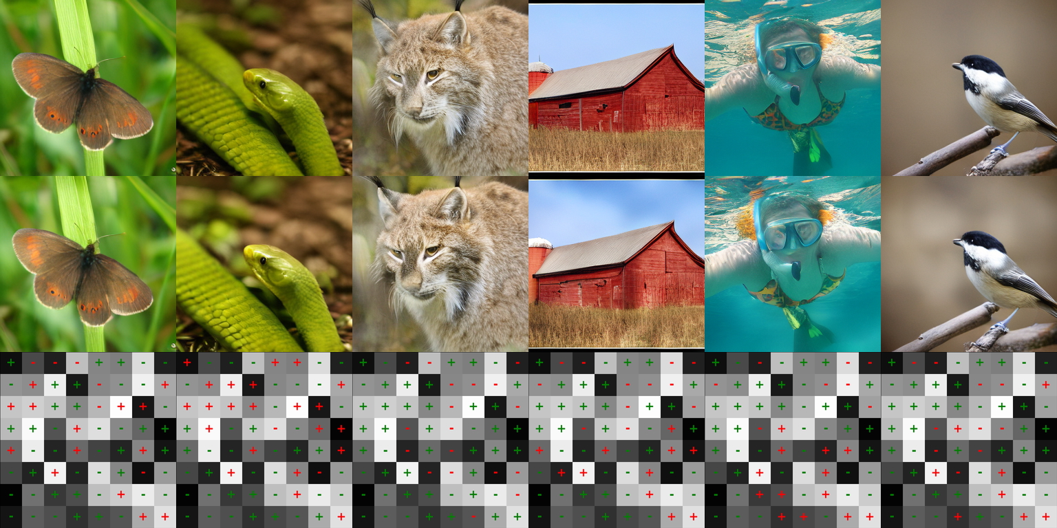
In Appendix 8, we present visualizations of watermarked and unwatermarked images generated by the nine models with the same seed as well as watermarked Stable Diffusion, revealing several interesting phenomena. First, in some cases (e.g., the first image in Figure [fig:var-d16]), our guidance induces only subtle modifications, such as minor variations in brightness or texture, to satisfy the watermark. In other cases (e.g., the third image in Figure [fig:edm2-xxl]), the model introduces additional objects to meet the constraint. This demonstrates that the models have sufficient capacity to adaptively and even creatively adjust the content to embed the watermark and maintain generation quality simultaneously.
Ablation Study
Luminark makes two key contributions: a novel watermark pattern and a general injection algorithm. An important question is whether either component could be substituted by conventional methods, and how each individually contributes to the overall success. In this subsection, we present ablation studies addressing this question and confirm that both components are essential.
Comparison I: Luminark’s watermark with other injection methods. We investigate whether watermark injection can be achieved through more straightforward approaches than guidance. To this end, we design two baseline methods: (i) post-hoc projection, which directly enforces a percentage of the luminance constraint only after the image has been fully generated; and (ii) hard step-wise projection, which forces a fixed percentage of patches to satisfy the constraint at every step of the generation process. We conduct our experiments on three representative models: EDM2-L, VAR-d30, and MAR-Large. As shown in Table [tab:ablation], both post-hoc projection and hard step-wise injection significantly degrade image quality as they introduce obvious block artifacts. In contrast, our guidance method enables the model to adaptively balance the two objectives, yielding high-quality outputs.
Comparison II: Guided injection with other watermarks. We investigate whether guidance can be combined with other watermark patterns to achieve performance comparable to Luminark. It is immediately clear that post-hoc watermarks discussed previously are bound to fail as they are non-robust, and diffusion-specific watermarks are incompatible. Luminark employs a specific linear combination of RGB values to construct the watermark. An interesting question is whether alternative combinations would also be effective. To investigate this, we design five variants: using only the R channel, only the G channel, only the R channel, the RGB average, as well as a random linear combination. Experiments are conducted on EDM2-L, VAR-d30, and MAR-Large. As shown in Table [tab:ablation], all alternatives lead to higher FID scores. This observation appears surprising, but can be partially understood from a perceptual perspective. Luminance has long been recognized as a dominant factor in image processing : principal component analyses consistently reveal that the first component of image data aligns closely with the perceptual notion of luminance. This intrinsic concentration of information in the luminance channel may explain why enforcing watermark constraints along this axis preserves generation quality more effectively than using arbitrary linear combinations of RGB values.
| With other watermark | With other injection method | |||||||
|---|---|---|---|---|---|---|---|---|
| (l0.5emr2em)3-7 (l-0.5emr-0em)8-9 Model | Luminark | R | G | B | Average | Random | Post-hoc | Hard Step-wise |
| EDM2-L | 2.72 | 3.01 | 3.39 | 4.30 | 3.48 | 3.03 | 16.70 | 92.05 |
| VAR-d30 | 3.06 | 3.08 | 3.26 | 3.74 | 3.32 | 3.52 | 7.68 | 33.25 |
| MAR-L | 3.32 | 3.50 | 3.49 | 4.89 | 3.41 | 4.06 | 6.88 | 85.15 |
Conclusions, Limitations, and Future Directions
In this work, we presented Luminark, a reliable and general watermarking method for vision generative models. By introducing a novel watermark pattern based on patch-level luminance statistics, Luminark provides a reliable detection mechanism with a statistical guarantee. To enable practical and model-agnostic watermark injection, we leveraged the widely adopted guidance technique and extended it into a plug-and-play watermark guidance framework. Comprehensive experiments demonstrate the effectiveness of our approach. According to our experience, the current version of Luminark has two limitations that can be addressed with further research. (a). The first limitation lies in the computational cost of generation, including the repeated sampling and additional backpropagation steps. We believe this issue can be mitigated through the use of a more effective penalty function and careful optimization, such as employing sparse WG updates or adopting early stopping strategies for WG when sufficient alignment has been achieved. (b). Secondly, we believe there remains room for further improvement in generation quality, particularly for MAR models. Potential solutions include adopting more fine-grained watermark patterns, as well as exploring adaptive guidance strategies.
Proof of Proposition 1
Proof. We introduce the auxiliary random variables $`Z_i=\mathbb{I}[\operatorname{sgn}(l(\mathbf{p}_i)-\tau_i)=c_i]`$, $`i=1,\cdots,N`$, so that $`m(\mathbf{x}, \mathcal{W})=\frac1N\sum_ {i=1}^N Z_i`$. We first show that the variables $`\{Z_i\}_{i=1}^N`$ are i.i.d and each follows a $`\operatorname{Bernoulli}(\frac{1}{2})`$ distribution with support $`\{0, 1\}`$. The independence follows directly from the fact that the variables $`\{c_i\}_{i=1}^N`$ are independently sampled. It is evident that the support of $`Z_i`$ is $`\{0,1\}`$, then we have $`\Pr(Z_i=1)=\Pr(c_i=\operatorname{sgn}(l(\mathbf{p}_i)-\tau_i))=\Pr(l(\mathbf{p}_i)\geq\tau_i)\Pr(c_i=1)+\Pr(l(\mathbf{p}_i)<\tau_i)\Pr(c_i=-1)=\frac{1}{2}l(\mathbf{p}_i) + \frac{1}{2}(1-l(\mathbf{p}_i))=\frac{1}{2}`$. Then we further have $`Pr(Z_i=0)=\frac{1}{2}`$, and the theorem yields by directly applying the Chernoff–Hoeffding theorem . ◻
Implementation of Image Transformations for Robust Detection
This appendix provides the Python code snippets used for the image manipulation attacks in our robustness evaluation. Each function takes a watermarked image as a NumPy array (in BGR channel order, as used by OpenCV) and returns the transformed image. The specific parameters used in our experiments are hardcoded in these functions for clarity and reproducibility.
Scaling
def scaling_attack(image: np.ndarray) -> np.ndarray:
    """Downscales to 96x96, then scales back to original size."""
    original_size = (image.shape[1], image.shape[0])
    downscaled = cv2.resize(image, (96, 96), interpolation=cv2.INTER_LINEAR)
    restored = cv2.resize(downscaled, original_size, interpolation=cv2.INTER_LINEAR)
return restoredCropping
def cropping_attack(image: np.ndarray) -> np.ndarray:
    """Crops a 2-pixel border and resizes back to original."""
    original_size = (image.shape[1], image.shape[0])
    # For a 512x512 image, this crops to a 510x510 region from (2,2)
    cropped = image[2:-2, 2:-2]
    restored = cv2.resize(cropped, original_size, interpolation=cv2.INTER_LINEAR)
return restoredJPEG Compression
def jpeg_compression_attack(image: np.ndarray) -> np.ndarray:
    """Applies JPEG compression with a quality factor of 50."""
    pil_image = Image.fromarray(cv2.cvtColor(image, cv2.COLOR_BGR2RGB))
    buffer = io.BytesIO()
    pil_image.save(buffer, format='JPEG', quality=50)
    buffer.seek(0)
    compressed_pil = Image.open(buffer)
    compressed_cv = cv2.cvtColor(np.array(compressed_pil), cv2.COLOR_RGB2BGR)
return compressed_cvFiltering (Median)
def filtering_attack(image: np.ndarray) -> np.ndarray:
    """Applies a median filter with an 11x11 kernel."""
return cv2.medianBlur(image, 11)Smoothing (Gaussian Blur)
def smoothing_attack(image: np.ndarray) -> np.ndarray:
    """Applies a Gaussian blur with a 9x9 kernel and sigma=15."""
return cv2.GaussianBlur(image, (9, 9), 15)Color Jitter
def color_jitter_attack(image: np.ndarray) -> np.ndarray:
    """Applies random color jitter with a factor of 0.1."""
    # Brightness, Saturation, Hue jitter in HSV space
    hsv = cv2.cvtColor(image, cv2.COLOR_BGR2HSV).astype(np.float32)
    hsv[:, :, 0] *= (1 + random.uniform(-0.1, 0.1)) # Hue
    hsv[:, :, 1] *= (1 + random.uniform(-0.1, 0.1)) # Saturation
    hsv[:, :, 2] *= (1 + random.uniform(-0.1, 0.1)) # Brightness
    np.clip(hsv[:, :, 0], 0, 179, out=hsv[:, :, 0])
    np.clip(hsv[:, :, 1:], 0, 255, out=hsv[:, :, 1:])
    jittered = cv2.cvtColor(hsv.astype(np.uint8), cv2.COLOR_HSV2BGR)

    # Contrast jitter using Pillow
    pil_img = Image.fromarray(cv2.cvtColor(jittered, cv2.COLOR_BGR2RGB))
    enhancer = ImageEnhance.Contrast(pil_img)
    contrast_factor = 1 + random.uniform(-0.1, 0.1)
    final_image = enhancer.enhance(contrast_factor)

return cv2.cvtColor(np.array(final_image), cv2.COLOR_RGB2BGR)Color Quantization
def color_quantization_attack(image: np.ndarray) -> np.ndarray:
    """Reduces the number of colors to 64 using k-means in CIELAB space."""
    lab_image = cv2.cvtColor(image, cv2.COLOR_BGR2LAB)
    pixel_data = np.float32(lab_image.reshape((-1, 3)))
    criteria = (cv2.TERM_CRITERIA_EPS + cv2.TERM_CRITERIA_MAX_ITER, 20, 1.0)
    _, labels, centers = cv2.kmeans(pixel_data, 64, None, criteria, 10, cv2.KMEANS_RANDOM_CENTERS)
    centers = np.uint8(centers)
    quantized_lab = centers[labels.flatten()].reshape(lab_image.shape)
return cv2.cvtColor(quantized_lab, cv2.COLOR_LAB2BGR)Gaussian Noise
def gaussian_noise_attack(image: np.ndarray) -> np.ndarray:
    """Adds Gaussian noise with mean=0 and std=25."""
    noise = np.random.normal(0, 25, image.shape)
    noisy_image = np.clip(image.astype(np.float32) + noise, 0, 255)
return noisy_image.astype(np.uint8)Sharpening
def sharpening_attack(image: np.ndarray) -> np.ndarray:
    """Applies an Unsharp Mask filter with radius=5 and strength=300%."""
    pil_image = Image.fromarray(cv2.cvtColor(image, cv2.COLOR_BGR2RGB))
    # 'percent' controls strength, 'threshold' is left at default
    sharpened = pil_image.filter(ImageFilter.UnsharpMask(radius=5, percent=300))
return cv2.cvtColor(np.array(sharpened), cv2.COLOR_RGB2BGR)Visualization of the Watermarked Images
For all the figures in this section, $`\mathcal{W}=(\mathbf{c},\boldsymbol{\tau})`$ is fixed within each experiment. Images generated by the vanilla pipeline are placed at the top, watermarked images with Luminark using the same seeds are placed in the middle, and visualization of $`\mathcal{W}=(\mathbf{c},\boldsymbol{\tau})`$ are placed at the bottom. In the bottom row, each cell corresponds to a patch: grayscale intensity encodes $`\tau`$ (lighter = larger luminance); +/– symbols denote $`c`$; symbol color indicates whether the luminance constraint is satisfied (green) or violated (red) in the corresponding watermarked image. Since Stable Diffusion is a diffusion-based model, it is naturally compatible with guidance. We directly extend our approach to the text-to-image scenario.

Guided Sampling for Latent Diffusion Models
Algorithm [alg:pixel_guided_sampler]
introduces a simple version of watermark injection for pixel-space
diffusion models. While effective, state-of-the-art diffusion models
typically operate in the latent space . In these models, the diffusion
process unfolds entirely in the latent domain, and the final image is
produced by a decoder network DEC that projects the latent
representation back into pixel space. It is easy to see that this
framework does not affect our watermark detection algorithm. However,
the generation procedure in
Algorithm [alg:pixel_guided_sampler]
requires adaptation. For latent diffusion models, at each sampling step
$`t`$, we decode the latent vector $`\mathbf{z}_t`$ into pixel space
using the decoder, enabling computation of the penalty term. Since the
mapping from a latent vector to its corresponding penalty value is
almost everywhere differentiable, we can still compute
$`\nabla_{\mathbf{z}_t} \text{Penalty}(\texttt{DEC}(\mathbf{z}_t), \mathcal{W})`$,
making the guidance possible. The full algorithm for Luminark applied to
latent diffusion models is provided in Algorithm
[alg:ldm_guided_sampler].
Input: Denoiser model $`D(\mathbf{z},\sigma)`$, Decoder DEC,
diffusion steps $`T`$, noise schedule $`\{\sigma_t\}_{t=0}^T`$,
watermark $`\mathcal{W}=(\mathbf{c}, \boldsymbol{\tau})`$, watermark
guidance scale $`s`$, threshold $`T_\text{match}`$ Initialize:
sample $`\mathbf{z}_T \sim \mathcal{N}(0, \sigma_T^2\mathbf{I})`$
$`\mathbf{z}_{t-1} \leftarrow \mathbf{z}_t - \left[ \underbrace{\frac{\mathbf{z}_t - D(\mathbf{z}_t,\sigma_t)}{\sigma_t}}_{\text{Denoising Term}} + \underbrace{s \nabla_{\mathbf{z}_t} \text{Penalty}(\texttt{DEC}(\mathbf{z}_t), \mathcal{W})}_{\text{Watermark Guidance Term}} \right] (\sigma_t - \sigma_{t-1})`$
$`\mathbf{x}_0 \leftarrow \texttt{DEC}(\mathbf{z}_0)`$
$`m \gets \frac{1}{N} \sum_{i=1}^{N} \mathbb{I}\!\left[\operatorname{sgn}(l(\mathbf{p}_i)-\tau_i)=c_i\right]`$
return $`\mathbf{x}_0`$
Guided Sampling for AR Models
Recent works, including the Vision Autoregressive Model (VAR) and Masked Autoregressive Model (MAR) , utilize guidance to enhance the quality of generation. For context, the autoregressive model can be generally formulated as:
\begin{equation}
    P(\mathbf{h}_1, \mathbf{h}_2, \cdots, \mathbf{h}_T)=\prod_{k=1}^T P(\mathbf{h}_t|\mathbf{h}_{<t}),
\end{equation}where $`\mathbf{h}_{ In the diffusion paradigm, Watermark Guidance is applied by modifying
the denoising term at every step to enforce the luminance constraint,
with its core idea being a step-wise modification procedure.
Autoregressive models also proceed sequentially, which allows any
guidance to be incorporated by adjusting the distribution
$`p(\mathbf{h}_t \mid \mathbf{h}_{ Input: Autoregressive model $`p`$, Decoder Input: Autoregressive model $`p`$, Decoder To the best of our knowledge, few studies have investigated watermarking
techniques on state-of-the-art autoregressive models, such as VAR and
MAR . Notable watermarking approaches are specifically designed for
diffusion models, such as recent Gaussian-Shading and the PRC
watermark . Therefore, we select these two methods as the baseline. Both and are developed upon the pioneer Tree-Ring approach. The core
principle of these methods is to inject a signature into the initial
noise during the diffusion process, and subsequently generate the
watermarked image by solving the Probability-Flow Ordinary Differential
Equation (ODE). The verification process leverages the diffeomorphism
property of the ODE: we can use an inverse ODE to reconstruct the
initial noise, thereby detecting the watermark’s presence. Specifically,
the signature in Gaussian Shading consists of noise samples drawn from
specific intervals of the Gaussian distribution, while that of PRC-W is
defined as the signs of the noise vector. From the description, we can
also easily see that this mechanism is specifically designed within the
diffusion paradigm and incompatible with other generative architectures. Compared with and , a key difference in our experimental setup is that
we generate a unique watermark for each method and keep it fixed
throughout the experiment. In contrast, the experimental setup in and
randomly generates a watermark on the fly for each image. Our setting is
evidently more practical, as a service provider can realistically
maintain only a limited number of keys, which makes reliable detection
feasible. By comparison, generating keys on the fly not only incurs
significant overhead in maintaining keys but also complicates detection.
A notable advantage of this alternative experimental design is that it
increases image diversity, which in turn yields substantially lower FID
scores. For completeness, we also replicated their experimental setting.
Empirically, we observe that the FIDs of all methods are similar and
close to the reference. We conduct experiments on three models from the EDM2 family: EDM2-XXL,
EDM2-L, and EDM2-XS. Each model is a latent diffusion model trained on
the ImageNet dataset, with images generated at a final resolution of
512$`\times`$512. All models in the EDM2 family utilize a U-Net architecture. For
EDM2-XXL, the number of channels is set to 448, and the number of
residual blocks per resolution in U-Net is set to 3, resulting in a
total of 3.05 billion parameters. For EDM2-L, the number of channels is
set to 320, and the number of blocks is set to 3, resulting in a total
of 1.56 billion parameters. For EDM2-XS, the number of channels is set
to 128, and the number of parameters is 0.25 billion. The diffusion
process is performed in the latent space, whose dimensionality is
$`64\times64\times4`$. Each image is first encoded into this space using
a VAE encoder. After the diffusion process, the latent representation is
projected back into the pixel space through the corresponding decoder. We conduct our experiments using the official open-source
implementation2 and the released pretrained checkpoints. For the
diffusion process, we follow the default configuration: the number of
diffusion steps is fixed at 32, with $`\sigma_{min}=0.002`$,
$`\sigma_{max}=80`$, and $`\rho=7`$, employing Heun’s second-order ODE
solver. For our watermark generator, the threshold $`\tau`$ is randomly
sampled from a uniform distribution $`U(0.4, 0.6)`$ to avoid extreme
values, and $`c`$ is randomly chosen from -1 and +1 with equal
probability. $`\tau`$ and $`c`$ are generated and then fixed during each
experiment. For watermark injection, the patch size is a key
hyperparameter. Choosing a patch size that is too small overly
constrains local flexibility, whereas an excessively large patch size
degrades detection performance. In all experiments, we therefore fix the
patch size to $`64\times64`$ for all models, and the total number of
patches is $`64`$. The watermark guidance scale ($`s`$) controls the
strength of the injection during the denoising process. For EDM2-XXL, we
set $`s`$ to be 34.375. For EDM2-L, we set $`s`$ to be 34.375. For
EDM2-XS, we set $`s`$ to be 34.375. To achieve a false positive rate
($`fpr`$) of 1%, we set match rate threshold $`T_{match}=0.61`$ using
Algorithm [alg:set_threshold_final]. We conduct experiments on three models from the VAR family: VAR-d36,
VAR-d30, and VAR-d16. Each model is a latent visual autoregressive model
trained on the ImageNet dataset, generating images at a final resolution
of 512$`\times`$512 for VAR-d36, and 256$`\times`$256
for VAR-d16 and VAR-d30. All models in the VAR family directly leverage GPT-2-like transformer
architecture . In VAR-d36, the embedding dimension is 2304, with 36
attention heads and 36 transformer layers, resulting in a total of 2.35
billion parameters. In VAR-d30, the embedding dimension is 1920, with 30
attention heads and 30 transformer layers, resulting in a total of 2.01
billion parameters. In VAR-d16, the embedding dimension is 1024, with 16
attention heads and 16 transformer layers, resulting in a total of 0.31
billion parameters. The generation process is performed in the latent
space, whose dimensionality is $`32\times32\times32`$ for VAR-d36, and
$`16\times16\times32`$ for VAR-d16 and VAR-d30. The resolution scales
used are $`\{1, 2, 3, 4, 6, 9, 13, 18, 24, 32\}`$ for VAR-36, while
$`\{1, 2, 3, 4, 5, 6, 8, 10, 13, 16\}`$ for VAR-16 and VAR-30. Each
image is first encoded into the latent space using a VQVAE encoder.
After the generation process, the latent representation is projected
back into pixel space through the corresponding decoder. We conduct our experiments using the official open-source checkpoint
3. Since only released a demo rather than the full sampling code, we
re-implemented their method for comparison. For our watermark generator,
the threshold $`\tau`$ is randomly sampled from a uniform distribution
$`U(0.4, 0.6)`$ to avoid extreme values, and $`c`$ is randomly chosen
from -1 and +1 with equal probability. $`\tau`$ and $`c`$ are generated
and then fixed during each experiment. For watermark injection, we fix
the total number of patches to $`64`$ for all models, resulting in a
patch size of $`64\times64`$ for VAR-36, while $`32\times32`$ for VAR-16
and VAR-30. Watermark injection is not applied at all scales. For VAR-16
and VAR-30, the watermark constraint is enforced at the last four
resolutions (8, 10, 13, and 16), whereas for VAR-36, the constraint is
applied only at the final resolution (32). The watermark guidance scale
is fixed at $`s=0.05`$ for VAR-16 and VAR-30. For VAR-36, since the
guidance is applied only at the final step, we adopt a gradient-descent
formulation with a reduced strength of $`s=0.015`$, optimizing over 8
steps. To achieve a false positive rate ($`fpr`$) of 1%, we set match
rate threshold $`T_{match}=0.625`$ using
Algorithm [alg:set_threshold_final]. We conduct experiments on three models from the MAR family: MAR-B,
MAR-L, and MAR-H. Each model is a latent autoregressive model trained on
the ImageNet dataset, with images generated at a final resolution of
256$`\times`$256. All models in the MAR family utilize a Transformer ViT architecture for
token embedding and an additional MLP for the diffusion procedure.
MAR-H, MAR-L, and MAR-B, respectively, have 40, 32, and 24 Transformer
blocks with a width of 1280, 1024, and 768. The denoising MLP,
respectively, has 12, 8, and 6 blocks and a width of 1536, 1280, and
1024. The generation process is performed in the latent space, whose
dimensionality is $`16\times16\times16`$. Each image is first encoded
into this space using a VAE encoder. After the generation process, the
latent representation is projected back into pixel space through the
corresponding decoder. We conduct our experiments using the official open-source implementation
4 and the released pretrained checkpoints. For the generation
process, we follow the default configuration: the number of
autoregressive steps is fixed at 256, and the diffusion sampling step is
set to $`100`$. For our watermark generator, the threshold $`\tau`$ is
randomly sampled from a uniform distribution $`U(0.4, 0.6)`$ to avoid
extreme values, and $`c`$ is randomly chosen from -1 and +1 with equal
probability. $`\tau`$ and $`c`$ are generated and then fixed during each
experiment. For watermark injection, the total number of patches is
fixed at $`64`$, yielding a patch size of $`32\times32`$, and the
guidance scale is set to $`s=0.015`$ across all models. To achieve a
false positive rate ($`fpr`$) of 1%, we set match rate threshold
$`T_{match}=0.61`$ using
Algorithm [alg:set_threshold_final]. In preparing this manuscript, we used ChatGPT (OpenAI) solely as a
writing assistant to improve the readability and fluency of the text.
Specifically, the model was employed to polish the language and refine
grammar without contributing to the conceptualization, methodology,
analysis, or results of this work. All ideas, experiments, and
conclusions are entirely the authors’ own.DEC, then
we can obtain
$`\nabla_{\mathbf{z}}\text{Penalty}(\texttt{DEC}(\mathbf{z}), \mathcal{W})`$.
Detailed procedures are outlined in
Algorithms [alg:watermark_var]
and [alg:watermark_mar], where
modifications to the original code are highlighted in blue.DEC, watermark pattern
$`\mathcal{W}=(\mathbf{c}, \boldsymbol{\tau})`$, watermark guidance
scale $`s`$, label $`y`$, resolution_scales (e.g.,
$`\{1,2,3,4,5,6,8,10,13,16\}`$), apply_constraint_steps (e.g.,
$`\{8,10,13,16\}`$), guidance steps $`S`$, threshold $`T_\text{match}`$
Initialize: $`\mathbf{z} \gets \text{embedding}(y)`$
$`\tilde{\mathbf{h}}_{t-1} \gets \text{interpolate}(\mathbf{z}, \text{resolution}\_\text{scales}[t-1])`$
Sample next token
$`\mathbf{h}_t \sim p(\mathbf{h}_t|\tilde{\mathbf{h}}_0,\tilde{\mathbf{h}}_1,\cdots,\tilde{\mathbf{h}}_{t-1})`$
$`\text{last\_scale} \gets \text{resolution}\_\text{scales}[-1]`$
$`\mathbf{z} \gets \mathbf{z} + \text{interpolate}(\mathbf{h}_t, \text{last\_scale})`$
$`\mathbf{z} \leftarrow \mathbf{z} - \nabla_{\mathbf{z}}\text{{Penalty}}(\texttt{DEC}(\mathbf{z}), \mathcal{W})`$
$`\mathbf{x} \leftarrow \texttt{DEC}(\mathbf{z})`$
$`m \gets \frac{1}{N} \sum_{i=1}^{N} \mathbb{I}\!\left[\operatorname{sgn}(l(\mathbf{p}_i)-\tau_i)=c_i\right]`$
return $`\mathbf{x}`$DEC, watermark pattern
$`\mathcal{W}=(\mathbf{c}, \boldsymbol{\tau})`$, watermark guidance
scale $`s`$, label $`y`$, ar_step $`T`$, threshold $`T_\text{match}`$
Initialize: $`\text{mask\_steps} \gets \text{gen\_mask\_order}(T)`$
Initialize: $`\mathbf{z} \gets \mathbf{0}`$
$`\text{mask\_to\_pred} \gets \text{mask\_steps[t]}`$ Sample next tokens
$`\mathbf{h}_t \sim p(\mathbf{h}_t|\mathbf{h}_1,\mathbf{h}_2,\cdots,\mathbf{h}_{t-1},y,\text{mask\_to\_pred})`$
$`\mathbf{z}[\text{mask\_to\_pred}] \gets \mathbf{h}_t`$
$`\mathbf{h}_t \leftarrow \mathbf{h}_t - \nabla_{\mathbf{h}_t}\text{{Penalty}}(\texttt{DEC}(\mathbf{z}), \mathcal{W})`$
$`\mathbf{z}[\text{mask\_to\_pred}] \gets \mathbf{h}_t`$
$`\mathbf{x} \leftarrow \texttt{DEC}(\mathbf{z})`$
$`m \gets \frac{1}{N} \sum_{i=1}^{N} \mathbb{I}\!\left[\operatorname{sgn}(l(\mathbf{p}_i)-\tau_i)=c_i\right]`$
return $`\mathbf{x}`$Description of Baseline Methods
Hyperparameters
EDM2 Hyperparameters
VAR Hyperparameters
MAR Hyperparameters
Use of Large Language Models (LLMs)
📊 논문 시각자료 (Figures)
A Note of Gratitude
The copyright of this content belongs to the respective researchers. We deeply appreciate their hard work and contribution to the advancement of human civilization.-
Since did not release the inference code for VAR, we re-implemented it ourselves. The results reported here are based on our reproduction, which differs slightly from the original paper. We refer to MAR as a hybrid as it uses autoregressive generation with diffusion heads. For completeness, we describe Gaussian-Shading and PRC-W in detail in Appendix 11. ↩︎