Learning from Historical Activations in Graph Neural Networks
📝 Original Paper Info
- Title: Learning from Historical Activations in Graph Neural Networks- ArXiv ID: 2601.01123
- Date: 2026-01-03
- Authors: Yaniv Galron, Hadar Sinai, Haggai Maron, Moshe Eliasof
📝 Abstract
Graph Neural Networks (GNNs) have demonstrated remarkable success in various domains such as social networks, molecular chemistry, and more. A crucial component of GNNs is the pooling procedure, in which the node features calculated by the model are combined to form an informative final descriptor to be used for the downstream task. However, previous graph pooling schemes rely on the last GNN layer features as an input to the pooling or classifier layers, potentially under-utilizing important activations of previous layers produced during the forward pass of the model, which we regard as historical graph activations. This gap is particularly pronounced in cases where a node's representation can shift significantly over the course of many graph neural layers, and worsened by graph-specific challenges such as over-smoothing in deep architectures. To bridge this gap, we introduce HISTOGRAPH, a novel two-stage attention-based final aggregation layer that first applies a unified layer-wise attention over intermediate activations, followed by node-wise attention. By modeling the evolution of node representations across layers, our HISTOGRAPH leverages both the activation history of nodes and the graph structure to refine features used for final prediction. Empirical results on multiple graph classification benchmarks demonstrate that HISTOGRAPH offers strong performance that consistently improves traditional techniques, with particularly strong robustness in deep GNNs.💡 Summary & Analysis
1. **Contribution 1: Self-Reflective Architectural Paradigm** GNNs can track node features across layers and integrate them to make more accurate predictions, much like a student analyzing past test results to prepare better for the next exam.-
Contribution 2: HistoGraph Mechanism
HistoGraph disentangles and models the layer-wise evolution of node embeddings and their spatial interactions, akin to applying multiple filters on an image to extract more information. -
Contribution 3: Performance Improvement Across Tasks
HistoGraph consistently outperforms state-of-the-art baselines in tasks such as graph-level classification, node classification, and link prediction, similar to a student who always scores the highest across various types of problems.
📄 Full Paper Content (ArXiv Source)
Introduction
Graph Neural Networks (GNNs) have achieved strong results on graph-structured tasks, including molecular property prediction and recommendation . Recent advances span expressive layers , positional and structural encodings , and pooling . However, pooling layers still underuse intermediate activations produced during message passing, limiting their ability to capture long-range dependencies and hierarchical patterns .
In GNNs, layers capture multiple scales: early layers model local neighborhoods and motifs, while deeper layers encode global patterns (communities, long-range dependencies, topological roles) , mirroring CNNs where shallow layers detect edges/textures and deeper layers capture object semantics . Greater depth can overwrite early information and cause over-smoothing, making node representations indistinguishable . We address this by leveraging historical graph activations, the representations from all layers, to integrate multi-scale features at readout .
Several works have explored the importance of deeper representations, residual connections, and expressive aggregation mechanisms to overcome such limitations . Close to our approach are specialized methods like state space and autoregressive moving average models on graphs, that consider a sequence of node features obtained by initialization techniques. Yet, these efforts often focus on improving stability during training, without explicitly modeling the internal trajectory of node features across layers. That is, we argue that a GNN’s computation path and the sequence of node features through layers can be a valuable signal. By reflecting on this trajectory, models can better understand which transformations were beneficial and refine their final predictions accordingly.
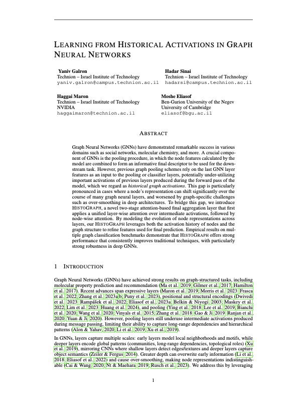
In this work, we propose HistoGraph, a self-reflective architectural paradigm that enables GNNs to reason about their historical graph activations. HistoGraph introduces a two-stage self-attention mechanism that disentangles and models two critical axes of GNN behavior: the evolution of node embeddings through layers, and their spatial interactions across the graph. The layer-wise module treats each node’s layer representations as a sequence and learns to attend to the most informative representation, while the node-wise module aggregates global context to form richer, context-aware outputs. HistoGraph design enables learning representations without modifying the underlying GNN architecture, leveraging the rich information encoded in intermediate representations to enhance many graph related predictions (graph classification, node classification and link prediction).
We apply HistoGraph in two complementary modes: (1) end-to-end joint training with the backbone, and (2) post-processing as a lightweight head on a frozen pretrained GNN. The end-to-end variant enriches intermediate representations, while the post-processing variant trains only the head, yielding substantial gains with minimal overhead. HistoGraph consistently outperforms strong GNN and pooling baselines on TU and OGB benchmarks , demonstrating that computational history is a powerful, general inductive bias. Figure 1 overviews HistoGraph.
Main contributions. (1) We introduce a self-reflective architectural paradigm for GNNs that leverages the full trajectory of node embeddings across layers; (2) We propose HistoGraph, a two-stage self-attention mechanism that disentangles the layer-wise node embeddings evolution and spatial aggregation of node features; (3) We empirically validate HistoGraph on graph-level classification, node classification and link prediction tasks, demonstrating consistent improvements over state-of-the-art baselines; and, (4) We show that HistoGraph can be employed as a post-processing tool to further enhance performance of models trained with standard graph pooling layers.
Related Works
r0.55
| Method |
|
|
|
|||||
|---|---|---|---|---|---|---|---|---|
| JKNet | Yes | No | No | |||||
| Set2Set | No | Yes | No | |||||
| SAGPool | No | Yes | No | |||||
| DiffPool | No | Yes | No | |||||
| SSRead | No | Yes | No | |||||
| DKEPool | No | Yes | No | |||||
| SOPool | No | Yes | No | |||||
| GMT | No | Yes | No | |||||
| Mean/Max/Sum Pool | No | No | No | |||||
| HistoGraph (Ours) | Yes | Yes | Yes |
Graph Neural Networks. GNNs propagate and aggregate messages along edges to produce node embeddings that capture local structure and features . GNN architectures are typically divided into two families: spectral GNNs, defining convolutions with the graph Laplacian (e.g., ChebNet , GCN ), and spatial GNNs, aggregating neighborhoods directly (e.g., GraphSAGE , GAT ). Greater GNN depth expands receptive fields but introduces over-smoothing and over-squashing . Mitigations include residual and skip connections , graph rewiring , and global context via positional encodings or attention (Graphormer , GraphGPS ). Several models preserve multi-hop information for robustness and expressivity. HistoGraph maintains node-embedding histories across propagation and fuses them at readout. Unlike per-layer mixing, this yields a consolidated multi-scale summary, mitigating intermediate feature degradation and retaining local and long-range information.
Pooling in Graph Learning. Graph-level tasks (e.g., molecular property prediction, graph classification) require a fixed-size summary of node embeddings. Early GNNs used permutation-invariant readouts such as sum, mean, and max , as in GIN . Richer structure motivated learned pooling: SortPool sorts embeddings and selects top-$`k`$ ; DiffPool learns soft clusters for hierarchical coarsening ; SAGPool scores nodes and retains a subset . Set2Set uses LSTM attention for iterative readout , while GMT uses multi-head attention for pairwise interactions . SOPool adds covariance-style statistics . A recent survey reviews flat and hierarchical techniques on TU and OGB benchmarks. Hierarchical approaches (e.g., Graph U-Net ) capture multi-scale structure but add complexity and risk information loss. In contrast, HistoGraph directly pools historical activations: layer-wise attention fuses multi-depth features, node-wise attention models spatial dependencies, and normalization stabilizes contributions. This preserves information across propagation depths without clustering or node dropping. Table [tab:pooling-methods] summarizes design choices and shows HistoGraph is the only method combining intermediate representations with structural information.
Residual Connections. Residuals are pivotal for deep GNNs and multi-scale features. Jumping Knowledge flexibly combines layers , APPNP uses personalized PageRank to preserve long-range signals , and GCNII adds initial residuals and identity mappings for stability . In pooling, Graph U-Net links encoder–decoder via skips , and DiffPool’s cluster assignments act as soft residuals preserving early-layer information . Other methods show that learnable residual connections can mitigate oversmoothing , and allow a dynamical system perspective on graphs . Differently, our HistoGraph departs by introducing historical pooling: at readout, it accumulates node histories across layers, creating a global shortcut at aggregation that revisits and integrates multi-hop features into the final representation unlike prior models that apply residuals only within node updates or via hierarchical coarsening.
Learning from Historical Graph Activations
We introduce HistoGraph, a learnable pooling operator that improves graph representation learning across downstream tasks by integrating layer evolution and spatial interactions in an end-to-end differentiable framework. Unlike pooling that operates on the last GNN layer, HistoGraph treats hidden representations as a sequence of historical activations. It computes node embeddings by querying each node’s history with its final-layer representation, then applies spatial self-attention to produce a fixed-size graph representation. Details appear in Appendix 8 and Algorithm [alg:method]; Figure 1 overviews HistoGraph, and Table [tab:pooling-methods] compares to other methods.
Notations. Let $`\mathbf{X} \in \mathbb{R}^{N \times L \times D_{\text{in}}}`$ be a batch of historical graph activations, where $`N`$ is the number of nodes in the batch, $`L`$ is the number of GNN layers or time steps, and $`D_{\text{in}}`$ is the feature dimensionality. Each node has $`L`$ historical embeddings corresponding to different depths of message passing. We assume that all GNN layers produce activations with the same dimensionality $`D_{\text{in}}`$.
We denote by $`\mathbf{X} = [\mathbf{X}^{(1)}, \ldots, \mathbf{X}^{(L-1)}]`$ the activation history of the GNN computations across $`L`$ layers. The initial representation is given by $`\mathbf{X}^{(0)} = \text{Emb}_{\text{in}}(\mathbf{F})`$, where $`\mathbf{F} \in \mathbb{R}^{N \times D_{\text{in}}}`$ is the input node features and $`\text{Emb}`$ is a linear layer. For each subsequent layer $`l = 1, \ldots, L-1`$, the representations are computed recursively as $`\mathbf{X}^{(l)} = \text{GNN}^{(l)}(\mathbf{X}^{(l-1)}),`$ where $`\text{GNN}^{(l)}`$ denotes the $`l`$-th GNN layer.
Input Projection and Per Layer Positional Encoding. We first project input features to a common hidden dimension $`D`$ using a linear transformation:
\begin{equation}
\mathbf{X}' = \text{Emb}_{\text{hist}}(\mathbf{X}) \in \mathbb{R}^{N \times L \times D}.
\end{equation}To encode layer ordering, we add fixed sinusoidal positional encodings as in :
\begin{equation}
\begin{aligned}
P_{l,2k} &= \sin\left(\frac{l}{10000^{2k/D}}\right),\quad
P_{l,2k+1} &= \cos\left(\frac{l}{10000^{2k/D}}\right),
\end{aligned}
\end{equation}for $`0 \le l < L`$, $`0 \le k < D/2`$, resulting in $`\mathbf{P} \in \mathbb{R}^{L \times D}`$, to obtain layer-aware features $`\widetilde{\mathbf{X}} = \mathbf{X}' + \mathbf{P}.`$
Layer-wise Attention and Node-wise Attention. We view each node through its sequence of historical activations and use attention to learn which activations are most relevant. We use only the last-layer embedding as the query to attend over all historical states:
\begin{equation}
\begin{aligned}
\mathbf{Q} &= \widetilde{\mathbf{X}}_{L-1}W^Q  \in \mathbb{R}^{N \times 1 \times D}, \quad
\mathbf{K} &= \widetilde{\mathbf{X}}W^K  \in \mathbb{R}^{N \times L \times D}, \quad
\mathbf{V} &= \widetilde{\mathbf{X}} \in \mathbb{R}^{N \times L \times D}.
\end{aligned}
\end{equation}We apply scaled dot-product attention and average across nodes, obtaining a layer weighting scheme:
\begin{equation}
\mathbf{c} = \operatorname{Average}\left( \frac{\mathbf{Q} \mathbf{K}^\top}{\sqrt{D}} \right) \in \mathbb{R}^{1 \times L}.
\end{equation}Rather than softmax, which enforces non-negative weights and suppresses negative differences, we apply a normalization that permits signed contributions $`\alpha_l = \frac{c_l}{\sum_{l'=0}^{L-1} c_{l'}}`$. This allows the model to express additive or subtractive relationships between layers, akin to finite-difference approximations in dynamical systems. The cross-layer pooled node embeddings are computed as:
\begin{equation}
\mathbf{H}
= \sum_{l=0}^{L-1} \alpha_l \cdot \widetilde{\mathbf{X}}_l
= \sum_{l=0}^{L-1} \frac{c_l}{\sum_{l'=0}^{L-1} c_{l'}} \cdot \widetilde{\mathbf{X}}_l
\;\;\in \mathbb{R}^{N \times D}.
\end{equation}Graph-level Representation. We first aggregate each node’s history weighted by relevance to the final state, with a residual recency bias from the final-layer query, into $`\mathbf{H}`$. Next, we obtain a graph-level representation by applying multi-head self-attention across nodes, omitting spatial positional encodings to preserve permutation invariance:
\begin{equation}
\mathbf{Z}=\mathrm{MHSA}(\mathbf{H},\mathbf{H},\mathbf{H})\in\mathbb{R}^{N\times D},
\end{equation}optionally followed by residual connections and LayerNorm. Averaging over nodes yields $`\mathbf{G}=\operatorname{Average}(\mathbf{Z})\in\mathbb{R}^{D}`$, which then feeds the final prediction head (typically an MLP). Early message-passing layers capture local interactions, whereas deeper layers encode global ones . By attending across layers and nodes, HistoGraph fuses local and global cues, retaining multi-scale structure and validating our motivation.
Computational Complexity. Layer-wise attention costs $`O(LD)`$ per node; spatial attention over $`N`$ nodes costs $`O(N^2D)`$. Thus the per-graph complexity is
\begin{equation}
O(NLD + N^2D)=O(N(L+N)D),
\end{equation}with memory $`O(L+N^2)`$ from attention maps. A naïve joint node–layer attention costs $`O(L^2N^2D)`$, which is prohibitive. Our two-stage scheme—first across layers ($`O(LD)`$ per node), then across nodes ($`O(N^2D)`$)—avoids this. Since $`L\ll N`$ in practice, the dominant cost is $`O(N^2D)`$, matching a single graph-transformer layer, whereas standard graph transformers stack $`L`$ such layers . This decomposition keeps historical activations tractable despite the quadratic node term. Empirically, HistoGraph adds only a slight runtime over a standard GNN forward pass (Figure 8) while delivering significant gains across multiple benchmarks, as seen in [tab:turesults,tab:ogb_results,tab:post-process-and-depth].
Frozen Backbone Efficiency. With a pretrained, frozen message-passing backbone, we train only the HistoGraph head. We cache the $`N \times L \times D`$ activations per graph in one forward pass and skip gradients through the backbone, removing $`O(L(ED + ND^2))`$ work (where $`E`$ is the number of edges). The backward pass applies only to the head, $`O(N(L + N)D)`$, substantially reducing memory and training time. This is especially useful in low-resource or few-shot regimes, and when fine-tuning large datasets where repeated backpropagation through $`L`$ GNN layers is prohibitive.
Properties of HistoGraph
In this section, we discuss the properties of our HistoGraph, which motivate its architectural design choices. In particular, these properties show how (i) layer-wise attention mitigates over-smoothing and acts as a dynamic trajectory filter, (ii) layer-wise attention can allow the architecture to approximate low/high pass filters, and (iii) node-wise attention is beneficial in our HistoGraph.
HistoGraph can mitigate Over-smoothing. One key property of HistoGraph is its ability to mitigate the over-smoothing problem in a simple way. As node embeddings tend to become indistinguishable after a certain depth $`l_{os}`$, i.e., $`|\mathbf{x}_v^{(l_1)} - \mathbf{x}_u^{(l_2)}| = 0`$ for all node pairs $`u,v`$ and layers $`l_1,l_2 \ge l_{os}`$, HistoGraph aggregates representations across layers using a weighted combination:
\begin{equation}
\mathbf{h_u} = \sum_{l=0}^{L-1} \alpha_l \mathbf{x_u}^{(l)}, \quad \text{with} \quad \sum_l \alpha_l = 1.
\end{equation}Attention weights $`\alpha_l`$ that place nonzero mass on early layers let the final embedding $`\mathbf{h}_u`$ retain discriminative early representations, countering over-smoothing so node embeddings remain distinguishable ($`|h_u - h_v|\neq 0`$). This mechanism underlies HistoGraph’s robustness in deep GNNs, corroborated by the depth ablation in Table 10 and by Fig. 4, which show substantial early-layer attention and nonzero differences between historical activations. We formalize HistoGraph’s mitigation of over-smoothing in 1; the proof appears in Appendix 11.
Proposition 1 (Mitigating Over-smoothing with HistoGraph). *Let $`\mathbf{x}_v^{(l)} \in \mathbb{R}^D`$ denote the embedding of node $`v`$ at layer $`l`$ of a GNN. Suppose the GNN exhibits over-smoothing, i.e., there exists some layer $`L_0`$ sufficiently large such that for all layers $`l_1, l_2 > L_0`$ and all nodes $`u,v`$,
\begin{equation}
\label{eq:oversmooth-def}
\|\mathbf{x}_u^{(l_1)} - \mathbf{x}_v^{(l_2)}\| \rightarrow 0.
\end{equation}
```*

*Let <span class="smallcaps">HistoGraph</span> compute the final node
embedding as
``` math
\begin{equation}
h_v = \sum_{l=0}^{L-1} \alpha_l \mathbf{x}_v^{(l)},
\end{equation}where $`\alpha_l`$ are learned attention weights. Then, for distinct nodes $`u`$ and $`v`$, there exists at least one layer $`l' \leq L_0`$ with $`\alpha_{l'} \neq 0`$ such that
\begin{equation}
\|h_u - h_v\| > 0.
\end{equation}
```*

*That is, <span class="smallcaps">HistoGraph</span> retains information
from early layers and mitigates over-smoothing.*

</div>

<figure id="fig:attention_and_embedding_evolution"
data-latex-placement="t">
<figure id="fig:layerwise_attention_scores">
<p><img src="/posts/2026/01/2026-01-03-190637-learning_from_historical_activations_in_graph_neur/combined_attention_visualization_IMDBB_64l.png"
alt="image" /> <span id="fig:layerwise_attention_scores"
data-label="fig:layerwise_attention_scores"></span></p>
</figure>
<figure id="fig:embedding_norm_diff">
<p><img src="/posts/2026/01/2026-01-03-190637-learning_from_historical_activations_in_graph_neur/combined_visualization_IMDBB_64l.png" alt="image" />
<span id="fig:embedding_norm_diff"
data-label="fig:embedding_norm_diff"></span></p>
</figure>
<figcaption>Visualizations on the <span class="smallcaps">imdb-b</span>
dataset with 64-layer <span class="smallcaps">HistoGraph</span>. (left)
Attention patterns across layers under different training regimes.
(right) Embedding evolution throughout training, measured by the normed
difference between final and intermediate representations.</figcaption>
</figure>

**<span class="smallcaps">HistoGraph</span>’s Layer-wise Attention is an
Adaptive Trajectory Filter.** <span id="prop:filter"
label="prop:filter"></span> We interpret
<span class="smallcaps">HistoGraph</span>’s layer-wise attention as an
Adaptive Trajectory Filter, which dynamically aggregates a node’s
embeddings across layers based on learned weights. Let
$`\{\mathbf{x}^{(l)}\}_{l=0}^{L-1} \subset \mathbb{R}^D`$ denote a
node’s embeddings at each layers. We define the aggregated embedding as:
``` math
\begin{equation}
\mathbf{h} = \sum_{l=0}^{L-1} \alpha_l \mathbf{x}^{(l)}, \quad \text{with} \quad \sum_l \alpha_l = 1.
\end{equation}where $`\alpha_l`$ are learnable attention weights. Depending on $`\alpha_l`$, the aggregation implements: (i) a low-pass filter when $`\alpha_l=\tfrac{1}{L}`$ (uniform average); (ii) a high-pass filter when $`\alpha_l=\delta_{l,L-1}-\delta_{l,L-2}`$ (first difference); and (iii) a general FIR filter when $`\alpha_l`$ are learned. Consequently, layer-wise attention in HistoGraph treats the GNN’s historical activations as a sequence and learns flexible, task-driven filtering and aggregation for the final classifier. Figure 5 illustrates a case where GCN fails at high-pass filtering, whereas HistoGraph succeeds. The barbell graph — a symmetric clique joined by a single edge—creates a sharp gradient discontinuity, highlighting how the adaptive filtering of HistoGraph preserves such signals, unlike standard GCNs. Appendix 10 further analyzes the usefulness of node-wise attention in HistoGraph.
 />
/>
 />
/>
 />
/>
 />
/>
Experiments
In this section, we conduct an extensive set of experiments to demonstrate the effectiveness of HistoGraph as a graph pooling function. Our experiments seek to address the following questions:
-
Does HistoGraph consistently improve GNN performance over existing pooling functions across diverse domains?
-
Can HistoGraph be applied as a post-processing step to enhance the performance of pretrained GNNs?
-
What is the impact of each component of HistoGraph on performance?
| Method $`\downarrow`$ / Dataset $`\rightarrow`$ | imdb-b | imdb-m | mutag | ptc | proteins | rdt-b | nci1 |
|---|---|---|---|---|---|---|---|
| SOPool | 78.5$`_{\pm2.8}`$ | 54.6$`_{\pm3.6}`$ | 95.3$`_{\pm4.4}`$ | 75.0$`_{\pm4.3}`$ | 80.1$`_{\pm2.7}`$ | 91.7$`_{\pm2.7}`$ | 84.5$`_{\pm 1.3}`$ |
| GMT | 79.5$`_{\pm 2.5}`$ | 55.0$`_{\pm2.8}`$ | 95.8$`_{\pm3.2}`$ | 74.5$`_{\pm4.1}`$ | 80.3$`_{\pm4.3}`$ | 93.9$`_{\pm 1.9}`$ | 84.1$`_{\pm2.1}`$ |
| HAP | 79.1$`_{\pm2.8}`$ | 55.3$`_{\pm 2.6}`$ | 95.2$`_{\pm2.8}`$ | 75.2$`_{\pm3.6}`$ | 79.9$`_{\pm4.3}`$ | 92.2$`_{\pm2.5}`$ | 81.3$`_{\pm1.8}`$ |
| PAS | 77.3$`_{\pm4.1}`$ | 53.7$`_{\pm3.1}`$ | 94.3$`_{\pm5.5}`$ | 71.4$`_{\pm3.9}`$ | 78.5$`_{\pm2.5}`$ | 93.7$`_{\pm 1.3}`$ | 82.8$`_{\pm2.2}`$ |
| HaarPool | 79.3$`_{\pm3.4}`$ | 53.8$`_{\pm3.0}`$ | 90.0$`_{\pm3.6}`$ | 73.1$`_{\pm5.0}`$ | 80.4$`_{\pm 1.8}`$ | 93.6$`_{\pm1.1}`$ | 78.6$`_{\pm0.5}`$ |
| GMN | 76.6$`_{\pm4.5}`$ | 54.2$`_{\pm2.7}`$ | 95.7$`_{\pm 4.0}`$ | 76.3$`_{\pm 4.3}`$ | 79.5$`_{\pm3.5}`$ | 93.5$`_{\pm0.7}`$ | 82.4$`_{\pm1.9}`$ |
| DKEPool | 80.9$`_{\pm 2.3}`$ | 56.3$`_{\pm 2.0}`$ | 97.3$`_{\pm 3.6}`$ | 79.6$`_{\pm 4.0}`$ | 81.2$`_{\pm 3.8}`$ | 95.0$`_{\pm 1.0}`$ | 85.4$`_{\pm 2.3}`$ |
| JKNet | 78.5$`_{\pm2.0}`$ | 54.5$`_{\pm2.0}`$ | 93.0$`_{\pm3.5}`$ | 72.5$`_{\pm2.0}`$ | 78.0$`_{\pm1.5}`$ | 91.5$`_{\pm2.0}`$ | 82.0$`_{\pm1.5}`$ |
| HistoGraph (Ours) | 87.2$`_{\pm 1.7}`$ | 61.9$`_{\pm 5.5}`$ | 97.9$`_{\pm 3.5}`$ | 79.1$`_{\pm 4.8}`$ | 97.8$`_{\pm 0.4}`$ | 93.4$`_{\pm0.9}`$ | 85.9$`_{\pm 1.8}`$ |
Baselines. We compare HistoGraph against diverse baselines spanning graph representation and pooling. Message-passing GNNs: GCN and GIN with mean or sum aggregation . Set-level pooling: Set2Set . Node-dropping pooling: SortPool , SAGPool , TopKPool , ASAP . Clustering-based pooling: DiffPool , MinCutPool , HaarPool , StructPool . EdgePool merges nodes along high-scoring edges. Attention-based global pooling: GMT . Additional models: SOPool , HAP , PAS , GMN , DKEPool , JKNet . On TUdatasets, we also include five kernel baselines: GK , RW , WL subtree , DGK , and AWE . An overview of baseline characteristics versus HistoGraph appears in Table [tab:pooling-methods].
Benchmarks. We use the OGB benchmark and the widely used TUDatasets ; dataset statistics appear in [tab:ogb-stats,tab:tudata-stats] in Appendix 7. For OGB, we follow with 3 GCN layers; for TUDatasets, we adopt , typically using 5 GIN layers. For deeper variants, we keep the backbone and vary the number of layers. Hyperparameters are in Appendix 9.1. Additionally, we benchmark HistoGraph on several node-classification datasets spanning heterophilic and homophilic graphs (Table 4) and across varying GNN depths (Table 1). Further results appear in Appendix 12: feature-distance across layers for GCN and GCN with HistoGraph (Table 5), comparison to the GraphGPS baseline (Table 7), and link prediction (Table 6).
$`^\dagger`$ symbolizes non-learnable methods.
| Method $`\downarrow`$ / Dataset $`\rightarrow`$ | molhiv | molbbbp | moltox21 | toxcast |
|---|---|---|---|---|
| GCN$`^\dagger`$ | 76.18$`_{\pm1.26}`$ | 65.67$`_{\pm1.86}`$ | 75.04$`_{\pm0.80}`$ | 60.63$`_{\pm0.51}`$ |
| GIN$`^\dagger`$ | 75.84$`_{\pm1.35}`$ | 66.78$`_{\pm1.77}`$ | 73.27$`_{\pm0.84}`$ | 60.83$`_{\pm0.46}`$ |
| MinCutPool | 75.37$`_{\pm2.05}`$ | 65.97$`_{\pm1.13}`$ | 75.11$`_{\pm0.69}`$ | 62.48$`_{\pm 1.33}`$ |
| GMT | 77.56$`_{\pm1.25}`$ | 68.31$`_{\pm 1.62}`$ | 77.30$`_{\pm 0.59}`$ | 65.44$`_{\pm 0.58}`$ |
| HAP | 75.71$`_{\pm1.33}`$ | 66.01$`_{\pm1.43}`$ | - | - |
| PAS | 77.68$`_{\pm 1.28}`$ | 66.97$`_{\pm1.21}`$ | - | - |
| DKEPool | 78.65$`_{\pm 1.19}`$ | 69.73$`_{\pm 1.51}`$ | - | - |
| HistoGraph (Ours) | 77.81$`_{\pm 0.89}`$ | 72.02$`_{\pm 1.46}`$ | 77.49$`_{\pm 0.70}`$ | 66.35$`_{\pm 0.80}`$ |
| Dataset | Method | 2 | 4 | 8 | 16 | 32 | 64 |
|---|---|---|---|---|---|---|---|
| Cora | GCN | 81.1 | 80.4 | 69.5 | 64.9 | 60.3 | 28.7 |
| GCN + HistoGraph | 81.3 | 82.9 | 80.7 | 83.1 | 80.6 | 77.5 | |
| Citeseer | GCN | 70.8 | 67.6 | 30.2 | 18.3 | 25.0 | 20.0 |
| GCN + HistoGraph | 70.9 | 69.5 | 69.9 | 69.3 | 67.2 | 63.4 | |
| Pubmed | GCN | 79.0 | 76.5 | 61.2 | 40.9 | 22.4 | 35.3 |
| GCN + HistoGraph | 78.9 | 78.2 | 78.6 | 80.4 | 80.0 | 79.3 |
Node classification accuracy (%) on benchmark datasets with varying GNN depth.
End-to-End Activation Aggregation with HistoGraph
We evaluate end-to-end activation aggregation with HistoGraph on graph-level benchmarks and node classification. We first report results on TUDatasets (Table [tab:turesults]), followed by OGB molecular property prediction (Table [tab:ogb_results]), and finally depth-scaled node classification (Table 1).
TUDatasets. On seven datasets (imdb-b, imdb-m, mutag, ptc, proteins, rdt-b, nci1), HistoGraph attains state-of-the-art performance on 5 of 7: imdb-b 87.2%, imdb-m 61.9%, mutag 97.9%, proteins 97.8%, nci1 85.9%. It is marginally behind on ptc at 79.1% versus 79.6% for DKEPool. Relative to the second-best method, gains are substantial on proteins (+16.6%), imdb-b (+6.3%), and imdb-m (+5.6%). Although DKEPool slightly leads on ptc and rdt-b, the overall trend favors HistoGraph across diverse graph classification benchmarks.
OGB molecular property prediction. On four OGB datasets (molhiv, moltox21, toxcast, molbbbp), HistoGraph achieves the top ROC-AUC on 3 of 4: molbbbp 72.02%, moltox21 77.49%, toxcast 66.35%. Margins over the second-best are +2.29% on molbbbp versus DKEPool, +0.91% on toxcast versus GMT, and +0.19% on moltox21 versus GMT. On molhiv, DKEPool leads with 78.65%, while HistoGraph is competitive at 77.81%, ranking in the top three, indicating strong generalization across molecular property prediction.
r0.25
| Dataset | Method | Acc. |
|---|---|---|
| imdb-m | MeanPool | 54.7 |
| FT | 67.3 | |
| Full FT | 62.7 | |
| End-to-End | 61.9 | |
| imdb-b | MeanPool | 76.0 |
| FT | 94.0 | |
| Full FT | 94.0 | |
| End-to-End | 87.2 | |
| proteins | MeanPool | 75.9 |
| FT | 97.3 | |
| Full FT | 97.3 | |
| End-to-End | 97.8 | |
| ptc | MeanPool | 77.1 |
| FT | 85.7 | |
| Full FT | 97.1 | |
| End-to-End | 88.6 |
Node classification. Table 1 shows that HistoGraph mitigates over-smoothing: standard GCN accuracy degrades with depth, whereas HistoGraph maintains stable, competitive performance up to 64 layers. This improves feature propagation while preserving discriminative power, particularly on heterophilic graphs. Additional node-classification results for heterophilic and homophilic datasets appear in Table 4 in Appendix 12.
Post-Processing of Trained GNNs with HistoGraph
We evaluate HistoGraph as a lightweight post-processing strategy on four TU graph-classification datasets: imdb-b, imdb-m, proteins, and ptc. For each dataset, we train GINs with 5, 16, 32, and 64 layers using standard architectures and mean pooling. After convergence, we save per-fold checkpoints and apply HistoGraph in three modes: (i) auxiliary head on a frozen backbone (HistoGraph(FT)), (ii) full joint fine-tuning (HistoGraph(Full FT)), and (iii) end-to-end training from scratch for comparison. Complete depth-wise results appear in Table 10 in Appendix 12.
Table [tab:post-process-best-depth] summarizes the graph-classification accuracy (%) across GIN depths for each dataset and method. HistoGraph used as a frozen auxiliary head (FT) consistently improves performance vs. MeanPool, often matching or surpassing full fine-tuning (Full FT) and end-to-end training. For example, on imdb-m, FT raises accuracy from 54.7% (MeanPool) to 67.3%; on imdb-b, both FT and Full FT reach 94.0%, far above the baseline (76.0%) and end-to-end (87.2%). On proteins, all HistoGraph variants achieve near-optimal performance, demonstrating effectiveness across datasets of varying size and characteristics. On ptc, Full FT attains the best score (97.1%), showing joint fine-tuning can further enhance results. Overall, HistoGraph offers a flexible, effective post-processing strategy that consistently boosts GNN performance.
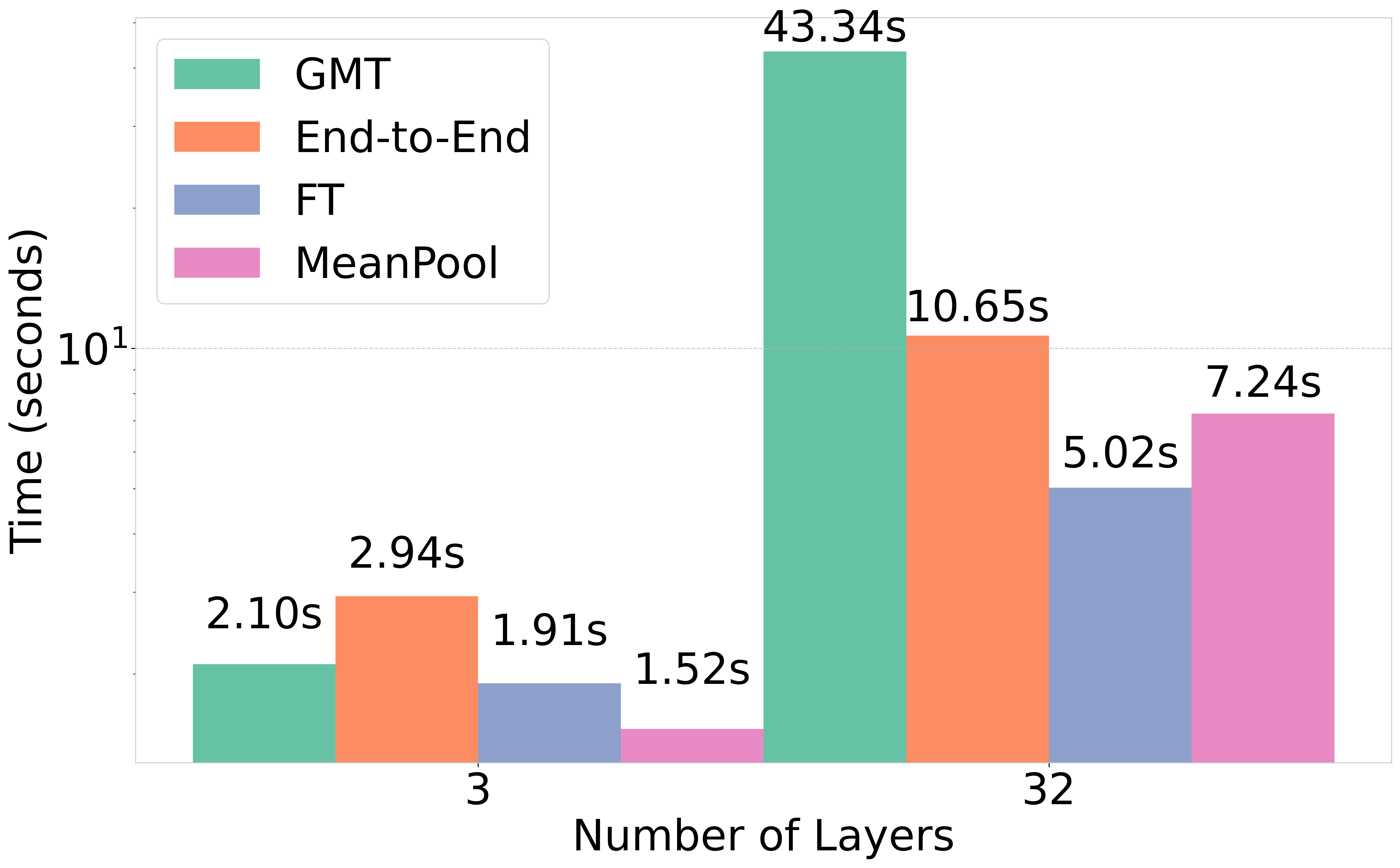
Runtime Analysis. We measure average training time per epoch for GCN backbones with 3 and 32 layers on molhiv and toxcast, comparing MeanPool, End-to-End, and FT. As shown in Fig. 8, End-to-End is costlier than MeanPool (e.g., 60.34s vs. 41.27s for 32 layers on molhiv) yet remains scalable. FT, which fine-tunes only the head on a pretrained MeanPool model, cuts overhead: training time is slightly higher for 3 layers but significantly lower for 32 layers on both datasets. While achieving results comparable to End-to-End (Table 10), FT offers an efficient way to boost existing models. Finally, HistoGraph is significantly faster than GMT in almost all cases, with larger speedups for deeper networks.

r0.45
| Variant | Acc. (%) | Std. |
|---|---|---|
| DKEPool | 81.20 | 3.80 |
| w/o Division by Sum | 74.45 | 6.28 |
| w/o Layer-wise Attention | 78.61 | 4.82 |
| w/o Node-wise Attention | 80.78 | 7.71 |
| HistoGraph (Ours) | 97.80 | 0.40 |
Ablation Study
Setup. We assess component contributions on the TUDatasets proteins dataset by removing or modifying parts and measuring classification accuracy (Table [tab:ablation]). We test three variants: (i) removing division-by-sum normalization, (ii) disabling layer-wise attention that models inter-layer dependencies, and (iii) disabling node-wise attention that captures cross-node dependencies.
Results and discussion. On proteins, HistoGraph attains 97.80% accuracy with a 0.40 standard deviation. Every ablation reduces accuracy; removing division-by-sum normalization performs worst at 74.45% $`\pm`$ 6.28, indicating each component is necessary. Removing layer-wise normalization allows attention weights to grow unbounded, destabilizing training and overshadowing early discriminative layers. Our signed normalization balances layer contributions and enables additive and subtractive filtering (Section 4), preserving discriminative information and stability. Against alternative aggregation strategies (mean aggregation and randomized attention), HistoGraph consistently outperforms them by a significant margin (Table 9, Appendix 12). Overall, normalization, layer-wise attention, and node-wise attention are critical for capturing complex dependencies and realizing the full performance of HistoGraph.
Conclusion
We introduced HistoGraph, a two-stage attention-based pooling layer that learns from historical activations to produce stronger graph-level representations. The design is simple and principled: layer-wise attention captures the evolution of each node’s trajectory across depths, node-wise self-attention models spatial interactions at readout, and signed layer-wise normalization balances contributions across layers to preserve discriminative signals and stabilize training. This combination mitigates over-smoothing and supports deeper GNNs while keeping computation and memory overhead modest. Across TU and OGB graph-level benchmarks, and in node-classification settings, HistoGraph consistently improves over strong pooling baselines and matches or surpasses leading methods on multiple datasets. Moreover, used as a lightweight post-processing head on frozen backbones, HistoGraph delivers additional gains without retraining the encoder. Taken together, the results establish intermediate activations as a valuable signal for readout and position HistoGraph as a practical, general drop-in pooling layer for modern GNNs.
Reproducibility Statement
To ensure reproducibility, we provide all code, model architectures, training scripts, and hyperparameter settings in a public repository (available upon acceptance). Dataset preprocessing, splits, and downsampling are detailed in Appendix 7. Hyperparameter configurations, including batch sizes, learning rates, hidden dimensions, and model depths, are documented in Appendix 9.1. Experiments were conducted using PyTorch and PyTorch Geometric on NVIDIA L40, A100, and GeForce RTX 4090 GPUs, with Weights and Biases for logging and model selection. All random seeds and training protocols are specified to facilitate replication.
Ethics Statement
Our work involves minimal ethical concerns. We use publicly available datasets (TU, OGB) that are widely adopted in graph learning research, adhering to their licensing terms. No private or sensitive data is introduced. Our method is primarily methodological, but we encourage responsible use to avoid potential misuse in applications that could impact privacy or enable harm. We acknowledge the environmental impact of large-scale training and note that HistoGraph’s computational efficiency may reduce energy costs compared to retraining full models.
Usage of Large Language Models in This Work
Large language models were used solely for minor text editing suggestions to improve clarity and grammar. All research concepts, code development, experimental design, and original writing were performed by the authors.
Dataset Statistics
Tables 2 and 3 summarize the statistics of the datasets used in our experiments. Table 2 covers molecular property prediction datasets from the Open Graph Benchmark (OGB), including molhiv, molbbbp, moltox21, and toxcast, reporting the number of graphs, number of prediction classes, and average number of nodes per graph. Table 3 presents the statistics of graph classification datasets from the TU benchmark suite, including social network datasets (imdb-b, imdb-m) and bioinformatics datasets (mutag, ptc, proteins, rdt-b, nci1). These datasets vary widely in graph sizes and label space, providing a comprehensive evaluation setting across small, medium, and large graphs with diverse class distributions.
| Dataset | molhiv | molbbbp | moltox21 | toxcast |
|---|---|---|---|---|
| # Graphs | 41,127 | 2,039 | 7,831 | 8,576 |
| # Classes | 2 | 2 | 12 | 617 |
| Nodes (avg.) | 25.51 | 24.06 | 18.57 | 18.78 |
Dataset statistics: number of graphs, number of classes, and average number of nodes.
| imdb-b | imdb-m | mutag | ptc | proteins | rdt-b | nci1 | ||
|---|---|---|---|---|---|---|---|---|
| # Graphs | 1000 | 1500 | 188 | 344 | 1113 | 2000 | 4110 | |
| # Classes | 2 | 3 | 2 | 2 | 2 | 2 | 2 | |
| Nodes(max) | 136 | 89 | 28 | 109 | 620 | 3783 | 111 | |
| Nodes(avg.) | 19.8 | 13.0 | 18.0 | 25.6 | 39.1 | 429.6 | 29.2 |
Implementation Details of HistoGraph
Algorithm [alg:method] outlines the forward pass of HistoGraph. The input $`\mathbf{X} \in \mathbb{R}^{N \times L \times D_\text{in}}`$ consists of node embeddings across $`L`$ GNN layers, for $`N`$ nodes per graph (referred to as historical graph activations). We first project the input to a common hidden dimension $`D`$ using a shared linear transformation. Sinusoidal positional encodings are added to encode the layer index. The final-layer embeddings serve as the query in an attention mechanism, while all intermediate layers act as key and value inputs. Attention scores are computed, averaged across nodes, and normalized over layers to yield a weighted aggregation of layer-wise features. A multi-head self-attention (MHSA) block is then applied over the aggregated node representations to capture spatial dependencies. Finally, a global average pooling operation over the node dimension produces the final graph-level representation $`\mathbf{Y} \in \mathbb{R}^D`$.
To stabilize training, we combined the output of HistoGraph with a simple mean pooling baseline using a learnable weighting factor $`\alpha \in [0, 1]`$. Specifically, the final graph representation was computed as a convex combination of the output of our method and the mean of the final-layer node embeddings: $`\mathbf{Y}_{\text{final}} = \alpha \cdot \mathbf{Y}_{\text{\textsc{HistoGraph}}} + (1 - \alpha) \cdot \mathbf{Y}_{\text{mean}}`$. We experimented both with fixed and learnable values of $`\alpha`$, and found that incorporating the mean-pooling signal helps guide the optimization in early training stages.
Input: $`\mathbf{X} \in \mathbb{R}^{N \times L \times D_\text{in}}`$ Output: Graph-level representation $`\mathbf{Y} \in \mathbb{R}^{D}`$ $`\mathbf{X}' \leftarrow \text{Emb}_{\text{hist}}(\mathbf{X})`$ $`\widetilde{\mathbf{X}} \leftarrow \mathbf{X}' + \mathbf{P}`$ $`\mathbf{Q} \leftarrow W^Q \widetilde{\mathbf{X}}_{L-1}`$ $`\mathbf{K} \leftarrow W^K \widetilde{\mathbf{X}}, \quad \mathbf{V} \leftarrow \widetilde{\mathbf{X}}`$ $`\mathbf{c} \leftarrow \frac{\mathbf{Q} \mathbf{K}^\top}{\sqrt{D}}`$ $`\mathbf{c} \leftarrow \operatorname{Average}(\mathbf{c})`$ $`\alpha_t \leftarrow \frac{c_t}{\sum_{t'} c_{t'}}`$ $`\mathbf{H} \leftarrow \sum_{t=0}^{L-1} \alpha_t \widetilde{\mathbf{X}}_t`$ $`\mathbf{Z} \leftarrow \mathrm{MHSA}(\mathbf{H}, \mathbf{H}, \mathbf{H})`$ $`\mathbf{Y} = \operatorname{Average}(\mathbf{Z})`$
Experimental Details
We implemented our method using PyTorch (offered under BSD-3 Clause license) and the PyTorch Geometric library (offered under MIT license). All experiments were run on NVIDIA L40, NVIDIA A100 and GeForce RTX 4090 GPUs. For logging, hyperparameter tuning, and model selection, we used the Weights and Biases (W&B) framework .
In the subsection below, we provide details on the hyperparameter configurations used across our experiments.
Hyperparameters
The hyperparameters in our method include the batch size $`B`$, hidden dimension $`D`$, learning rate $`l`$, and weight decay $`\gamma`$. We also tune architectural and attention-specific components such as the number of attention heads $`H`$, use of fully connected layers, inclusion of zero attention token, use of layer normalization, and skip connections. Attention dropout rates are controlled via the multi-head attention dropout $`p_{\text{mha}}`$ and attention mask dropout $`p_{\text{mask}}`$. We further include the use of a learning rate schedule as a hyperparameter. Additionally, we consider different formulations for the attention coefficient parameterization $`\alpha_{\text{type}}`$, including learnable, fixed, and gradient-constrained variants. Hyperparameters were selected via a combination of grid search and Bayesian optimization, using validation performance as the selection criterion. For baseline models, we consider the search space of their relevant hyperparameters.
Additional Properties of HistoGraph
Contribution of Node-wise Attention for Graph-Level Prediction. Let $`\mathbf{H} = [\mathbf{h}_1, \dots, \mathbf{h}_N] \in \mathbb{R}^{N \times D}`$ be the cross-layer-pooled node embeddings. Suppose the downstream task requires a function $`f: \mathbb{R}^{N \times D} \to \mathbb{R}^K`$ that is permutation-invariant but non-uniform (e.g., depends on inter-node interactions). Then, standard mean pooling cannot approximate $`f`$ unless it includes additional inter-node operations like node-wise attention.
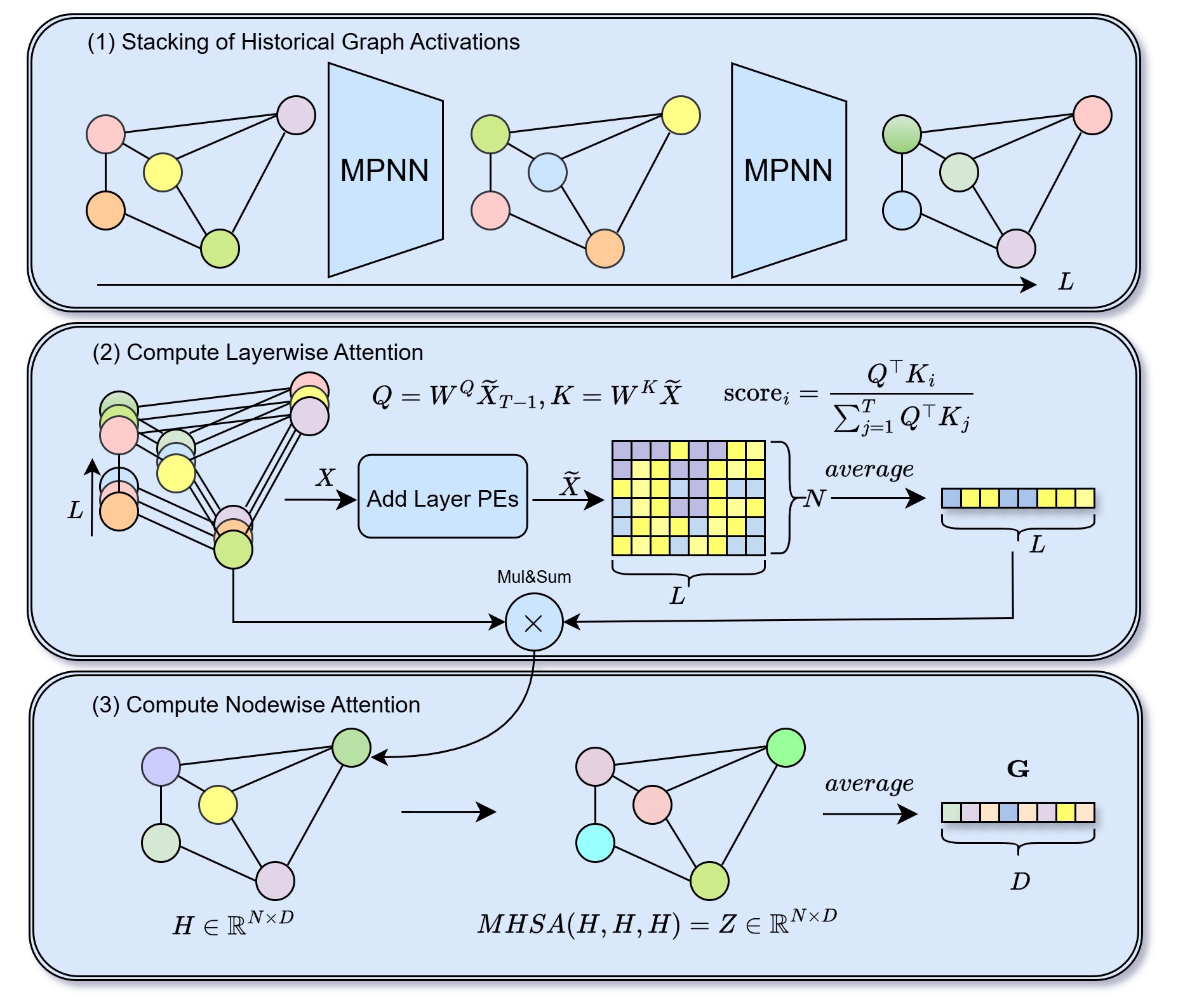
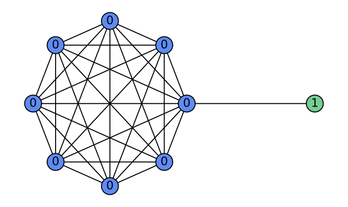
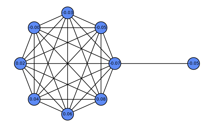
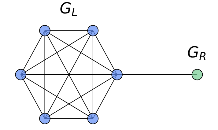
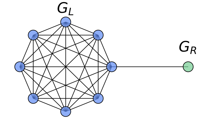
As a concrete example where the node-wise attention is beneficial in our HistoGraph, let us consider a graph $`G = (V, E)`$ composed of two subgraphs connected by a narrow bridge. Let $`G_L = (V_L, E_L)`$ be a large graph $`G(n, p)`$ with $`n \gg 1`$, and let $`G_R = (V_R, E_R)`$ be a singleton graph containing a single node $`v_R`$. The resulting structure is illustrated in Figure 9.
Suppose the graph-level classification task depends solely on the features of the singleton node $`v_R`$ (e.g., label is determined by a property encoded in $`v_R`$). In this setting, a naive mean pooling aggregates all node embeddings uniformly. As $`n`$ increases, the contribution of $`v_R`$ to the pooled representation becomes increasingly marginal, leading to its signal being dominated by the embeddings from the much larger subgraph $`G_L`$. This becomes especially problematic when there is a distribution shift at test time, e.g., $`G_L`$ becomes larger or denser, which further suppresses the contribution of $`v_R`$.
In contrast, a node-wise attention mechanism can learn to attend selectively to $`v_R`$, regardless of the size of $`G_L`$, making it robust to distributional changes. This demonstrates the contribution of node-wise attention in capturing non-uniform importance of nodes in our HistoGraph.
 />
/>
 />
/>
Proofs
HistoGraph mitigates oversmoothing
Proof.
Consider two nodes $`u`$ and $`v`$. Under the definition of HistoGraph’s final embedding:
\begin{equation}
h_u - h_v = \sum_{l=0}^{L-1} \alpha_l \left( \mathbf{x}_u^{(l)} - \mathbf{x}_v^{(l)} \right).
\end{equation}We split the sum into layers before and after $`L_0`$:
\begin{align}
h_u - h_v
&= \sum_{l=0}^{L_0} \alpha_l \left( \mathbf{x}_u^{(l)} - \mathbf{x}_v^{(l)} \right)
+ \sum_{l=L_0+1}^{L-1} \alpha_l \left( \mathbf{x}_u^{(l)} - \mathbf{x}_v^{(l)} \right).
\end{align}By over-smoothing (Eq. [eq:oversmooth-def]), for all $`l > L_0`$:
\begin{equation}
\| \mathbf{x}_u^{(l)} - \mathbf{x}_v^{(l)} \| \approx 0,
\end{equation}and hence the second sum is negligible. Therefore,
\begin{equation}
h_u - h_v \approx \sum_{l=0}^{L_0} \alpha_l \left( \mathbf{x}_u^{(l)} - \mathbf{x}_v^{(l)} \right).
\end{equation}Because initial node representations differ (a standard assumption for distinct nodes), there exists at least one layer $`l' \leq L_0`$ for which
\begin{equation}
\| \mathbf{x}_u^{(l')} - \mathbf{x}_v^{(l')} \| \neq 0.
\end{equation}Given that HistoGraph employs learned dynamic attention, suppose $`\alpha_{l'} \neq 0`$. Consequently:
\begin{align}
\| h_u - h_v \|
&\approx \left\| \alpha_{l'} \left( \mathbf{x}_u^{(l')} - \mathbf{x}_v^{(l')} \right)
+ \sum_{l \neq l'} \alpha_l \left( \mathbf{x}_u^{(l)} - \mathbf{x}_v^{(l)} \right) \right\| \\
&> 0.
\end{align}This directly contradicts the assumption that node embeddings become indistinguishable in the pooled representation. Thus, HistoGraph mitigates over-smoothing by explicitly retaining discriminative early-layer representations.
Additional Experiments
Table [tab:full_turesults] and Table [tab:full_ogb_results] show the results of different methods on two different settings of multiple graph pooling methods. Table 4 reports node classification accuracy on both heterophilic and homophilic datasets. We observe that our method (HistoGraph+ GCN) consistently outperforms standard GCN and JKNet across all datasets. The improvements are particularly pronounced on heterophilic graphs such as Actor, Squirrel, and Chameleon, where our method achieves gains of up to 12.3% over GCN. On homophilic datasets like Cora, Citeseer, and Pubmed, we also observe consistent, albeit smaller, improvements.
| Method $`\downarrow`$ / Dataset $`\rightarrow`$ | imdb-b | imdb-m | mutag | ptc | proteins | rdt-b | nci1 |
|---|---|---|---|---|---|---|---|
| Kernel | |||||||
| GK | 65.9$`_{\pm1.0}`$ | 43.9$`_{\pm0.4}`$ | 81.4$`_{\pm1.7}`$ | 57.3$`_{\pm1.4}`$ | 71.7$`_{\pm0.6}`$ | 77.3$`_{\pm0.2}`$ | 62.3$`_{\pm0.3}`$ |
| RW | - | - | 79.2$`_{\pm2.1}`$ | 57.9$`_{\pm1.3}`$ | 74.2$`_{\pm0.4}`$ | - | - |
| WL | 73.8$`_{\pm3.9}`$ | 50.9$`_{\pm3.8}`$ | 82.1$`_{\pm0.4}`$ | 60.0$`_{\pm0.5}`$ | 74.7$`_{\pm0.5}`$ | - | 82.2$`_{\pm0.2}`$ |
| DGK | 67.0$`_{\pm0.6}`$ | 44.6$`_{\pm0.5}`$ | - | 60.1$`_{\pm2.6}`$ | 75.7$`_{\pm0.5}`$ | 78.0$`_{\pm0.4}`$ | 80.3$`_{\pm0.5}`$ |
| AWE | 74.5$`_{\pm5.9}`$ | 51.5$`_{\pm3.6}`$ | 87.9$`_{\pm9.8}`$ | - | - | 87.9$`_{\pm2.5}`$ | - |
| GNN | |||||||
| ASAP | 77.6$`_{\pm2.1}`$ | 54.5$`_{\pm2.1}`$ | 91.6$`_{\pm5.3}`$ | 72.4$`_{\pm7.5}`$ | 78.3$`_{\pm4.0}`$ | 93.1$`_{\pm2.1}`$ | 75.1$`_{\pm1.5}`$ |
| SOPool | 78.5$`_{\pm2.8}`$ | 54.6$`_{\pm3.6}`$ | 95.3$`_{\pm4.4}`$ | 75.0$`_{\pm4.3}`$ | 80.1$`_{\pm2.7}`$ | 91.7$`_{\pm2.7}`$ | 84.5$`_{\pm 1.3}`$ |
| GMT | 79.5$`_{\pm 2.5}`$ | 55.0$`_{\pm2.8}`$ | 95.8$`_{\pm3.2}`$ | 74.5$`_{\pm4.1}`$ | 80.3$`_{\pm4.3}`$ | 93.9$`_{\pm 1.9}`$ | 84.1$`_{\pm2.1}`$ |
| HAP | 79.1$`_{\pm2.8}`$ | 55.3$`_{\pm 2.6}`$ | 95.2$`_{\pm2.8}`$ | 75.2$`_{\pm3.6}`$ | 79.9$`_{\pm4.3}`$ | 92.2$`_{\pm2.5}`$ | 81.3$`_{\pm1.8}`$ |
| PAS | 77.3$`_{\pm4.1}`$ | 53.7$`_{\pm3.1}`$ | 94.3$`_{\pm5.5}`$ | 71.4$`_{\pm3.9}`$ | 78.5$`_{\pm2.5}`$ | 93.7$`_{\pm 1.3}`$ | 82.8$`_{\pm2.2}`$ |
| HaarPool | 79.3$`_{\pm3.4}`$ | 53.8$`_{\pm3.0}`$ | 90.0$`_{\pm3.6}`$ | 73.1$`_{\pm5.0}`$ | 80.4$`_{\pm 1.8}`$ | 93.6$`_{\pm1.1}`$ | 78.6$`_{\pm0.5}`$ |
| DiffPool | 73.9$`_{\pm3.6}`$ | 50.7$`_{\pm2.9}`$ | 94.8$`_{\pm4.8}`$ | 68.3$`_{\pm5.9}`$ | 76.2$`_{\pm3.1}`$ | 91.8$`_{\pm2.1}`$ | 76.6$`_{\pm1.3}`$ |
| GMN | 76.6$`_{\pm4.5}`$ | 54.2$`_{\pm2.7}`$ | 95.7$`_{\pm 4.0}`$ | 76.3$`_{\pm 4.3}`$ | 79.5$`_{\pm3.5}`$ | 93.5$`_{\pm0.7}`$ | 82.4$`_{\pm1.9}`$ |
| DKEPool | 80.9$`_{\pm 2.3}`$ | 56.3$`_{\pm 2.0}`$ | 97.3$`_{\pm 3.6}`$ | 79.6$`_{\pm 4.0}`$ | 81.2$`_{\pm 3.8}`$ | 95.0$`_{\pm 1.0}`$ | 85.4$`_{\pm 2.3}`$ |
| JKNet | 78.5$`_{\pm2.0}`$ | 54.5$`_{\pm2.0}`$ | 93.0$`_{\pm3.5}`$ | 72.5$`_{\pm2.0}`$ | 78.0$`_{\pm1.5}`$ | 91.5$`_{\pm2.0}`$ | 82.0$`_{\pm1.5}`$ |
| HistoGraph (Ours) | 87.2$`_{\pm 1.7}`$ | 61.9$`_{\pm 5.5}`$ | 97.9$`_{\pm 3.5}`$ | 79.1$`_{\pm 4.8}`$ | 97.8$`_{\pm 0.4}`$ | 93.4$`_{\pm0.9}`$ | 85.9$`_{\pm 1.8}`$ |
$`^\dagger`$ symbolizes non-learnable methods.
| Method $`\downarrow`$ / Dataset $`\rightarrow`$ | molhiv | molbbbp | moltox21 | toxcast |
|---|---|---|---|---|
| GCN$`^\dagger`$ | 76.18$`_{\pm1.26}`$ | 65.67$`_{\pm1.86}`$ | 75.04$`_{\pm0.80}`$ | 60.63$`_{\pm0.51}`$ |
| GIN$`^\dagger`$ | 75.84$`_{\pm1.35}`$ | 66.78$`_{\pm1.77}`$ | 73.27$`_{\pm0.84}`$ | 60.83$`_{\pm0.46}`$ |
| HaarPool$`^\dagger`$ | 74.69$`_{\pm1.62}`$ | 66.11$`_{\pm0.82}`$ | - | - |
| ASAP | 72.86$`_{\pm1.40}`$ | 63.50$`_{\pm2.47}`$ | 72.24$`_{\pm1.66}`$ | 58.09$`_{\pm1.62}`$ |
| TopKPool | 72.27$`_{\pm0.91}`$ | 65.19$`_{\pm2.30}`$ | 69.39$`_{\pm2.02}`$ | 58.42$`_{\pm0.91}`$ |
| SortPool | 71.82$`_{\pm1.63}`$ | 65.98$`_{\pm1.70}`$ | 69.54$`_{\pm0.75}`$ | 58.69$`_{\pm1.71}`$ |
| JKNet | 74.99$`_{\pm1.60}`$ | 65.62$`_{\pm0.77}`$ | 65.98$`_{\pm0.46}`$ | - |
| SAGPool | 74.56$`_{\pm1.69}`$ | 65.16$`_{\pm1.93}`$ | 71.10$`_{\pm1.06}`$ | 59.88$`_{\pm0.79}`$ |
| Set2Set | 74.70$`_{\pm1.65}`$ | 66.79$`_{\pm1.05}`$ | 74.10$`_{\pm1.13}`$ | 59.70$`_{\pm1.04}`$ |
| SAGPool(H) | 71.44$`_{\pm1.67}`$ | 63.94$`_{\pm2.59}`$ | 69.81$`_{\pm1.75}`$ | 58.91$`_{\pm0.80}`$ |
| EdgePool | 72.66$`_{\pm1.70}`$ | 67.18$`_{\pm1.97}`$ | 73.77$`_{\pm0.68}`$ | 60.70$`_{\pm0.92}`$ |
| MinCutPool | 75.37$`_{\pm2.05}`$ | 65.97$`_{\pm1.13}`$ | 75.11$`_{\pm0.69}`$ | 62.48$`_{\pm 1.33}`$ |
| StructPool | 75.85$`_{\pm1.81}`$ | 67.01$`_{\pm2.65}`$ | 75.43$`_{\pm0.79}`$ | 62.17$`_{\pm1.61}`$ |
| SOPool | 76.98$`_{\pm1.11}`$ | 65.82$`_{\pm1.66}`$ | - | - |
| GMT | 77.56$`_{\pm1.25}`$ | 68.31$`_{\pm 1.62}`$ | 77.30$`_{\pm 0.59}`$ | 65.44$`_{\pm 0.58}`$ |
| HAP | 75.71$`_{\pm1.33}`$ | 66.01$`_{\pm1.43}`$ | - | - |
| PAS | 77.68$`_{\pm 1.28}`$ | 66.97$`_{\pm1.21}`$ | - | - |
| DiffPool | 75.64$`_{\pm1.86}`$ | 68.25$`_{\pm0.96}`$ | 74.88$`_{\pm0.81}`$ | 62.28$`_{\pm0.56}`$ |
| GMN | 77.25$`_{\pm1.70}`$ | 67.06$`_{\pm1.05}`$ | - | - |
| DKEPool | 78.65$`_{\pm 1.19}`$ | 69.73$`_{\pm 1.51}`$ | - | - |
| HistoGraph (Ours) | 77.81$`_{\pm 0.89}`$ | 72.02$`_{\pm 1.46}`$ | 77.49$`_{\pm 0.70}`$ | 66.35$`_{\pm 0.80}`$ |
| Dataset | GCN | JKNet | HistoGraph+ GCN (Ours) |
|---|---|---|---|
| Actor | 27.3 $`\pm`$ 1.1 | 35.1 $`\pm`$ 1.4 | 36.2 $`\pm`$ 1.1 |
| Squirrel | 53.4 $`\pm`$ 2.0 | 45.0 $`\pm`$ 1.7 | 65.7 $`\pm`$ 1.4 |
| Chameleon | 64.8 $`\pm`$ 2.2 | 63.8 $`\pm`$ 2.3 | 69.8 $`\pm`$ 1.8 |
| Cora | 81.1 $`\pm`$ 0.8 | 81.0 $`\pm`$ 1.0 | 83.1 $`\pm`$ 0.4 |
| Citeseer | 70.8 $`\pm`$ 0.7 | 69.8 $`\pm`$ 0.8 | 70.9 $`\pm`$ 0.5 |
| Pubmed | 79.0 $`\pm`$ 0.6 | 78.1 $`\pm`$ 0.5 | 80.4 $`\pm`$ 0.4 |
Node classification accuracy (mean $`\pm`$ std) on heterophilic and homophilic datasets.
To evaluate the ability of HistoGraph to mitigate oversmoothing, we measure the feature distance across layers for a standard GCN, both with and without HistoGraph. The results, presented in Table 5, show that incorporating HistoGraph consistently leads to higher feature distances across all layers, with the most pronounced improvement observed in the pre-classifier layer as expected due to the oversmoothing.
The results in Tables 6–8 further demonstrate the versatility and effectiveness of HistoGraph across different tasks and architectures. On the OGBL-COLLAB link prediction benchmark (Table 6), incorporating HistoGraph as a readout function leads to consistent improvements over a standard GCN baseline. Similarly, in molecular property prediction tasks with GraphGPS backbones (Table 7), HistoGraph achieves substantial performance gains across multiple datasets, highlighting its ability to preserve and leverage historical information across layers. Finally, the ablation on the number of historical layers (Table 8) shows that incorporating deeper historical context enhances predictive performance, with the best results obtained when more layers are retained. These findings underscore the robustness of HistoGraph as a drop-in replacement for readout functions across diverse settings. Finally, we present an additional ablation in Table 9, which examines the effect of different aggregation strategies across all layers—mean aggregation, randomized attention, and HistoGraph. Across datasets, HistoGraph consistently achieves superior performance.
| Layer | 0 | 8 | 64 | Final (pre-classifier) |
|---|---|---|---|---|
| GCN | 2.634 | 2.385 | 1.703 | 1.703 |
| GCN + HistoGraph | 3.710 | 3.403 | 2.888 | 5.000 |
Feature distance metrics across layers, showing the ability of HistoGraph to mitigate oversmoothing. Compared to standard GCN, HistoGraph yields more diverse node embeddings.
| Model | Hits@50 (Test) ↑ | Hits@50 (Validation) ↑ |
|---|---|---|
| Baseline (GCN) | 0.4475 $`\pm`$ 0.0107 | 0.5263 $`\pm`$ 0.0115 |
| GCN + HistoGraph | 0.4533 $`\pm`$ 0.0096 | 0.5314 $`\pm`$ 0.0103 |
Link prediction results on the OGBL-COLLAB dataset. HistoGraph is applied as a drop-in replacement for the readout function with a GCN backbone, demonstrating consistent improvements over the baseline.
| Method | PROTEINS | tox21 | ToxCast |
|---|---|---|---|
| GPS + MeanPool | 79.8 $`\pm`$ 2.1 | 75.7 $`\pm`$ 0.4 | 62.5 $`\pm`$ 1.09 |
| GPS + HistoGraph | 98.9 $`\pm`$ 1.2 | 77.8 $`\pm`$ 2.2 | 66.9 $`\pm`$ 0.69 |
Performance comparison of GraphGPS baselines with and without HistoGraph on multiple datasets. Integrating HistoGraph consistently improves performance by preserving layer-wise historical context and enabling adaptive readout.
| #Historical Layers | PTC (%) |
|---|---|
| 5 | $`79.1 \pm 4.8`$ |
| 3 | $`75.6 \pm 3.7`$ |
| 1 | $`73.8 \pm 4.3`$ |
Performance of HistoGraph with different numbers of historical layers on PTC.
| Dataset | Mean over all layers | Randomized attention | HistoGraph |
|---|---|---|---|
| imdb-multi | 54.73 $`\pm`$ 2.3 | 54.73 $`\pm`$ 4.3 | 61.9 $`\pm`$ 5.5 |
| imdb-binary | 75.5 $`\pm`$ 2.2 | 76.6 $`\pm`$ 1.4 | 87.2 $`\pm`$ 1.7 |
| proteins | 70.08 $`\pm`$ 5.8 | 80.05 $`\pm`$ 3.2 | 97.8 $`\pm`$ 0.4 |
| ptc | 73.24 $`\pm`$ 3.2 | 73.56 $`\pm`$ 2.56 | 79.1 $`\pm`$ 4.8 |
Comparison between different aggregation options of all layers: mean over all layers, randomized attention, and HistoGraph performance across datasets.
| Dataset | Method | Number of Layers | |||
|---|---|---|---|---|---|
| 3-6 | 5 | 16 | 32 | 64 | |
| imdb-m | MeanPool | 54.0 | 54.7 | 52.0 | 52.0 |
| FT | 67.3 | 64.7 | 57.3 | 66.0 | |
| Full FT | 58.0 | 62.7 | 58.0 | 57.3 | |
| End-to-End | 61.9 | 58.7 | 58.7 | 54.7 | |
| imdb-b | MeanPool | 76.0 | 76.0 | 76.0 | 71.0 |
| FT | 94.0 | 84.0 | 81.0 | 78.0 | |
| Full FT | 94.0 | 81.0 | 81.0 | 81.0 | |
| End-to-End | 87.2 | 79.0 | 79.0 | 72.0 | |
| proteins | MeanPool | 75.0 | 75.0 | 75.0 | 75.9 |
| FT | 97.3 | 77.7 | 75.9 | 77.8 | |
| Full FT | 97.3 | 84.8 | 80.4 | 97.3 | |
| End-to-End | 97.8 | 78.6 | 84.8 | 94.6 | |
| ptc | MeanPool | 77.1 | 68.6 | 71.4 | 68.5 |
| FT | 85.7 | 80.0 | 71.5 | 71.4 | |
| Full FT | 85.7 | 97.1 | 82.9 | 80.0 | |
| End-to-End | 79.1 | 88.6 | 85.7 | 80.0 | |
Scalable Post-Processing with HistoGraph
Table 10 indicates that all HistoGraph variants consistently outperform the MeanPool baseline for every depth and dataset. In particular, FT, often matches or even exceeds the accuracy of full end‐to‐end tuning despite having far fewer trainable parameters. For example, at 5 layers it boosts imdb-m from 54.0 % to 67.3 %, imdb-b accuracy from 76.0 % to 94.0 %, proteins from 75.0 % to 97.3 %, and ptc from 77.1 % to 85.7 %. As model depth grows, FT remains highly competitive: at 16 layers it achieves 64.7%.
We would like to note that while HistoGraph mitigates over-smoothing by dynamically leveraging early-layer discriminative features, at extreme depths (e.g., 64 layers) we face known optimization challenges in GNNs . Nonetheless, HistoGraph consistently outperforms baseline pooling methods, as shown in our depth-varying experiments on Cora, Citeseer, and Pubmed in Table 1, demonstrating robustness to model depth.
These findings demonstrate that caching intermediate representations and training a small auxiliary head enables scalable, modular adaptation of GNNs, obtaining strong performance across depths and domains without incurring the computational costs of full model training.
📊 논문 시각자료 (Figures)