Improved Object-Centric Diffusion Learning with Registers and Contrastive Alignment
📝 Original Paper Info
- Title: Improved Object-Centric Diffusion Learning with Registers and Contrastive Alignment- ArXiv ID: 2601.01224
- Date: 2026-01-03
- Authors: Bac Nguyen, Yuhta Takida, Naoki Murata, Chieh-Hsin Lai, Toshimitsu Uesaka, Stefano Ermon, Yuki Mitsufuji
📝 Abstract
Slot Attention (SA) with pretrained diffusion models has recently shown promise for object-centric learning (OCL), but suffers from slot entanglement and weak alignment between object slots and image content. We propose Contrastive Object-centric Diffusion Alignment (CODA), a simple extension that (i) employs register slots to absorb residual attention and reduce interference between object slots, and (ii) applies a contrastive alignment loss to explicitly encourage slot-image correspondence. The resulting training objective serves as a tractable surrogate for maximizing mutual information (MI) between slots and inputs, strengthening slot representation quality. On both synthetic (MOVi-C/E) and real-world datasets (VOC, COCO), CODA improves object discovery (e.g., +6.1% FG-ARI on COCO), property prediction, and compositional image generation over strong baselines. Register slots add negligible overhead, keeping CODA efficient and scalable. These results indicate potential applications of CODA as an effective framework for robust OCL in complex, real-world scenes.💡 Summary & Analysis
1) **Register-augmented slot diffusion**. CODA introduces register slots that are independent of the input image, acting as attention sinks to absorb residual attention and keep object slots focused on meaningful associations. 2) **Mitigating text-conditioning bias**. By fine-tuning key, value, and output projections in cross-attention layers, CODA reduces biases inherited from pre-trained diffusion models, ensuring more accurate slot-image alignment. 3) **Contrastive alignment objective**. A contrastive loss ensures slots capture concepts present in the image, improving overall representation quality by maximizing mutual information between inputs and slots.📄 Full Paper Content (ArXiv Source)
Introduction
Object-centric learning (OCL) aims to decompose complex scenes into structured, interpretable object representations, enabling downstream tasks such as visual reasoning , causal inference , world modeling , robotic control , and compositional generation . Yet, learning such compositional representations directly from images remains a core challenge. Unlike text, where words naturally form composable units, images lack explicit boundaries for objects and concepts. For example, in a street scene with pedestrians, cars, and traffic lights, a model must disentangle these entities without labels and also capture their spatial relations (e.g., a person crossing in front of a car). Multi-object scenes add further complexity: models must not only detect individual objects but also capture their interactions. As datasets grow more cluttered and textured, this becomes even harder. Manual annotation of object boundaries or compositional structures is costly, motivating the need for fully unsupervised approaches such as Slot Attention (SA) . While effective in simple synthetic settings, SA struggles with large variations in real-world images, limiting its applicability to visual tasks such as image or video editing.
Combining SA with diffusion models has recently pushed forward progress in OCL . In particular, Stable-LSD and SlotAdapt achieve strong object discovery and high-quality generation by leveraging pretrained diffusion backbones such as Stable Diffusion (SD). Nevertheless, these approaches still face two key challenges. First, as illustrated in 1 (left), they often suffer from slot entanglement, where a slot encodes features from multiple objects or fragments of them, leading to unfaithful single-slot generations. This entanglement degrades segmentation quality and prevents composable generation to novel scenes and object configurations. Second, they exhibit weak alignment, where slots fail to consistently correspond to distinct image regions, especially on real-world images. As shown in our experiments, slots often suffer from over-segmentation (splitting one object into multiple slots), under-segmentation (merging multiple objects into one slot), or inaccurate object boundaries. Together, these two issues reduce both the accuracy of object-centric representations and their utility for compositional scene generation.
In response, we propose Contrastive Object-centric Diffusion
Alignment (CODA), a slot-attention model that uses a pretrained
diffusion decoder to reconstruct the input image. CODA augments the
model with register slots, which absorb residual attention and reduce
interference between object slots, and a contrastive objective, which
explicitly encourages slot–image alignment. As illustrated
in 1 (right), CODA faithfully
generates images from both individual slots as well as their
compositions. In summary, the contributions of this paper can be
outlined as follows.
-
Register-augmented slot diffusion. We employ register slots that are independent of the input image into slot diffusion. Although these register slots carry no semantic information, they act as attention sinks, absorbing residual attention mass so that semantic slots remain focused on meaningful object–concept associations. This reduces interference between object slots and mitigating slot entanglement (4.1).
-
Mitigating text-conditioning bias. To reduce the influence of text-conditioning biases inherited from pretrained diffusion models, we finetune the key, value, and output projections in cross-attention layers. This adaptation further improves alignment between slots and visual content, ensuring more faithful object-centric decomposition (4.2).
-
Contrastive alignment objective. We propose a contrastive loss that ensures slots capture concepts present in the image (4.3). Together with the denoising loss, our training objective can be viewed as a tractable surrogate for maximizing the mutual information (MI) between inputs and slots, improving slot representation quality (4.4).
-
Comprehensive evaluation. We demonstrate that
CODAoutperforms existing unsupervised diffusion-based approaches across synthetic and real-world benchmarks in object discovery (5.1), property prediction (5.2), and compositional generation (5.3). On the VOC dataset,CODAimproves instance-level object discovery by +3.88% mBO$`^i`$ and +3.97% mIoU$`^i`$, and semantic-level object discovery by +5.72% mBO$`^c`$ and +7.00% mIoU$`^c`$. On the COCO dataset, it improves the foreground Adjusted Rand Index (FG-ARI) by +6.14%.
 style="width:49.0%" />
style="width:49.0%" />
style="width:49.0%" />
Related work
Object-centric learning (OCL). The goal of OCL is to discover compositional object representations from images, enabling systematic generalization and stronger visual reasoning . Learning directly from raw pixels is difficult, so previous works leveraged weak supervision (e.g., optical flow , depth , text , pretrained features ), or auxiliary losses that guide slot masks toward moving objects . Scaling OCL to complex datasets has been another focus: DINOSAUR reconstructed self-supervised features to segment real-world images, and FT-DINOSAUR extended this via encoder finetuning for strong zero-shot transfer. SLATE and STEVE combined discrete VAE tokenization with slot-conditioned autoregressive transformers, while SPOT improved autoregressive decoders using patch permutation and attention-based self-training. Our work builds on SA, but does not require any additional supervision.
Diffusion models for OCL. Recent works explored diffusion models as
slot decoders in OCL. Different methods vary in how diffusion models are
integrated. For example, SlotDiffusion trained a diffusion model from
scratch, while Stable-LSD , GLASS , and SlotAdapt leveraged pretrained
diffusion models. Although pretrained models offer strong generative
capabilities, they are often biased toward text-conditioning. To address
this issue, GLASS employed cross-attention masks as pseudo-ground truth
to guide SA training. Unlike GLASS, CODA does not rely on supervised
signals such as generated captions. SlotAdapt introduced adapter layers
to enable new conditional signals while keeping the base diffusion model
frozen. In contrast, CODA simply finetunes key, value, and output
projections in cross-attention, without introducing additional layers.
This ensures full compatibility with off-the-shelf diffusion models
while remaining conceptually simple and computationally efficient.
Contrastive learning for OCL. Training SA with only reconstruction
losses often leads to unstable or inconsistent results . To improve
robustness, several works introduced contrastive objectives. For
example, SlotCon applied the InfoNCE loss across augmented views of
the input image to enforce slot consistency. used contrastive loss to
enforce the temporal consistency for video object-centric models. In
contrast, CODA tackles compositionality by aligning images with their
slot representations, enabling faithful generation from both individual
slots and their combinations. Unlike , who explicitly maximize
likelihood under random slot mixtures and thus directly tune for
compositional generation, CODA focuses on enforcing slot–image
alignment; its gains in compositionality arise indirectly from improved
disentanglement. Although CODA uses a negative loss term, similar to
negative guidance in diffusion models , the roles are fundamentally
different. apply negative guidance during sampling to steer the
denoising trajectory, whereas CODA uses a contrastive loss during
training to improve slot–image alignment.
Background
Slot Attention (SA). Given input features $`{\mathbf{f}}\in \mathbb{R}^{M\times D_\mathrm{input}}`$ of an image, the goal of OCL is to extract a sequence $`{\mathbf{s}}\in \mathbb{R}^{N \times D_{\mathrm{slot}}}`$ of $`N`$ slots, where each slot is a $`D_{\mathrm{slot}}`$-dimensional vector representing a composable concept. In SA, we start with randomly initialized slots as $`{\mathbf{s}}^{(0)} \in \mathbb{R}^{N\times D_\mathrm{slot}}`$. Once initialized, SA employs an iterative mechanism to refine the slots. In particular, slots serve as queries, while the input features serve as keys and values. Let $`q`$, $`k`$, and $`v`$ denote the respective linear projections used in the attention computation. Given the current slots $`{\mathbf{s}}^{(t)}`$ and input features $`{\mathbf{f}}`$, the update rule can be formally described as
\begin{align*}
    {\mathbf{s}}^{(t + 1)} = \mathtt{GRU} ({\mathbf{s}}^{(t)}, {{\mathbf{u}}^{(t)}}) \quad \text{where} \quad {\mathbf{u}}^{(t)} = \mathtt{Attention}(q({\mathbf{s}}^{(t)}), k({\mathbf{f}}), v({\mathbf{f}})) \,. %\rvm^{(t)}=\mathtt{softmax}(q(\rvs^{(t)})\dot k(\rvf)^\top/\,.
\end{align*}Here, attention readouts are aggregated and refined through a Gated Recurrent Unit (GRU). Unlike self-attention , the $`\mathtt{softmax}`$ function in SA is applied along the slot axis, enforcing competition among slots. This iterative process is repeated for several steps, and the slots from the final iteration are taken as the slot representations. Finally, these slots are passed to a decoder trained to reconstruct the input image. The slot decoder can take various forms, such as an MLP or an autoregressive Transformer . Interestingly, recent works have shown that using (latent) diffusion models as slot decoders proves to be particularly powerful and effective in OCL.
Latent diffusion models (LDMs). Diffusion models are probabilistic models that sample data by gradually denoising Gaussian noise . The forward process progressively corrupts data with Gaussian noise, while the reverse process learns to denoise and recover the original signal. To improve efficiency, SD performs this process in a compressed latent space rather than pixel space. Concretely, a pretrained autoencoder maps an image to a latent vector $`{\mathbf{z}}\in \mathcal{Z}`$, where a U-Net denoiser iteratively refines noisy latents. Consider a variance preserving process that mixes the signal $`{\mathbf{z}}`$ with Gaussian noise $`{\boldsymbol{\epsilon}}\sim \mathcal{N}(0, \mathbf{I})`$, given by $`{\mathbf{z}}_\gamma = \sqrt{\sigma(\gamma)} {\mathbf{z}}+ \sqrt{\sigma(-\gamma)} {\boldsymbol{\epsilon}}`$, where $`\sigma(.)`$ is the sigmoid function and $`\gamma`$ is the log signal-to-noise ratio. Let $`{\boldsymbol{\epsilon}}_{\boldsymbol{\theta}}({\mathbf{z}}_\gamma, \gamma, {\mathbf{c}})`$ denote a denoiser parameterized by $`{\boldsymbol{\theta}}`$ that predicts the Gaussian noise $`{\boldsymbol{\epsilon}}`$ from noisy latents $`{\mathbf{z}}_\gamma`$, conditioned on an external signal $`{\mathbf{c}}`$. In SD, conditioning is implemented through cross-attention, which computes attention between the conditioning signal and the features produced by U-Net. Training diffusion models is formulated as a noise prediction problem, where the model learns to approximate the true noise $`{\boldsymbol{\epsilon}}`$ added during the forward process,
\begin{align*}
    \min_{{\boldsymbol{\theta}}} \quad \mathbb{E}_{({\mathbf{z}}, {\mathbf{c}}), {\boldsymbol{\epsilon}}, \gamma} \left[ \| {\boldsymbol{\epsilon}}- {\boldsymbol{\epsilon}}_{\boldsymbol{\theta}}({\mathbf{z}}_\gamma, \gamma, {\mathbf{c}})\|^2_2 \right] \,
\end{align*}with $`({\mathbf{z}}, {\mathbf{c}})`$ sampled from a data distribution $`p({\mathbf{z}}, {\mathbf{c}})`$. Once training is complete, sampling begins from random Gaussian noise, which is iteratively refined using the trained denoiser.
Proposed method
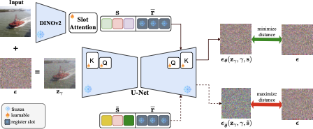
As summarized in 2, CODA builds on diffusion-based
OCL by extracting slot sequences from DINOv2 features with SA and
decoding them using a pretrained SD v1.5 . To address the challenges of
slot entanglement and weak alignment, CODA introduces three
components: (i) register slots to absorb residual attention and keep
object slots disentangled, (ii) finetuning of cross-attention keys and
queries to mitigate text-conditioning bias, and (iii) a contrastive
alignment loss to explicitly align images with their slots. These
modifications yield disentangled, well-aligned slots that enable
faithful single-slot generation and compositional editing.
 style="width:90.0%" />
CODA. The input
image is encoded with DINOv2 and processed by Slot Attention (SA) to
produce slot representations. The semantic slots s, together with register
slots $\overline{{\mathbf{r}}}$, serve
as conditioning inputs for the cross-attention layers of a pretrained
diffusion model. SA is trained jointly with the key, value, and output
projections of the cross-attention layers using a denoising objective
that minimizes the mean squared error between the true and predicted
noise. In addition, a contrastive loss is applied to align each image
with its corresponding slot representations.Register slots
An ideal OCL model should generate semantically faithful images when conditioned on arbitrary subsets of slots. In practice, however, most diffusion-based OCL methods fall short of this goal. As discussed in the introduction, decoding a single slot typically yields distorted or semantically uninformative outputs. Although reconstructions from the full set of slots resemble the input images, this reliance reveals a strong interdependence among slots (see 4 for more detailed analysis). Such slot entanglement poses a challenge for compositionality, particularly when attempting to reuse individual concepts in novel configurations.
To address this problem, we add input-independent register slots that act as residual attention sinks, absorbing shared or background information and preventing object slots from mixing. Intuitively, register slots are semantically empty but structurally valid inputs, making them natural placeholders for slots that can capture residual information without competing with object representations. We obtain these register slots by passing only padding tokens through the SD text encoder, a pretrained ViT-L/14 CLIP . Formally, let $`\texttt{pad}`$ denote the padding token used to ensure fixed-length prompts in text-to-image SD. By encoding the sequence $`[\texttt{pad}, \dots, \texttt{pad}]`$ with the frozen text encoder1, we obtain a fixed-length sequence of frozen embeddings serving as register slots $`\overline{{\mathbf{r}}}`$. We also explore an alternative design with trainable register slots in 5.2, and find that while learnable registers can also mitigate slot entanglement, our simple fixed registers perform best.
Why do register slots mitigate slot entanglement? The $`\mathtt{softmax}`$ operation in cross-attention forces attention weights to sum to one across all slots. When a query from U-Net features does not strongly match any semantic slot, this constraint causes the attention mass to spread arbitrarily, weakening slot–concept associations. Register slots serve as placeholders that absorb this residual attention, giving the model extra capacity to store auxiliary information without interfering with semantic slots. This leads to cleaner and more coherent slot-to-concept associations. Consistent with this view, we observe in 3 that a substantial fraction of attention mass is allocated to register slots. A similar phenomenon has been reported in language models, where $`\mathtt{softmax}`$ normalization causes certain initial tokens to act as attention sinks , absorbing unnecessary attention mass and preventing it from distorting meaningful associations.
In a related approach, introduced an additional embedding by pooling from either generated slots or image features. Unlike our method, their embedding is injected directly into the cross-attention layers and is explicitly designed to capture global scene information. While this might provide contextual guidance, it ties the model to input-specific features, reducing flexibility in reusing slots across arbitrary compositions. In contrast, our register slots are independent of the input image, making them better suited for compositional generation.
Finetuning cross-attention keys and queries
SD is trained on large-scale image–text pairs, so directly using its pretrained model as a slot decoder introduces a text-conditioning bias: the model expects text embeddings and tends to prioritize language-driven semantics over slot-level representations . This mismatch weakens the fidelity of slot-based generation. Prior works have approached this issue in different ways. For example, trained diffusion models from scratch, thereby removing text bias but sacrificing generative quality due to limited training data. More recently, proposed adapter layers to align slot representations with pretrained diffusion models, retaining generation quality but still relying on text-conditioning features.
In contrast, we adopt a lightweight adaptation strategy: finetuning only the key, value, and output projections in cross-attention layers . This allows the model to better align slots with visual content, mitigating text-conditioning bias while preserving the expressive power of the pretrained diffusion backbone. We find this minimal modification sufficient to eliminate the bias introduced by text conditioning. Unlike the previous approaches, our method is both computationally and memory efficient, requiring no additional layers or architectural modifications. This makes our approach not only effective but also conceptually simple. Formally, let $`{\boldsymbol{\phi}}`$ denote the parameters of SA, the denoising objective for diffusion models can be written as
\begin{align}
    \mathcal{L}_{\mathrm{dm}} ({\boldsymbol{\phi}}, {\boldsymbol{\theta}}) = \mathbb{E}_{({\mathbf{z}}, {\mathbf{s}}), {\boldsymbol{\epsilon}}, \gamma} \left[ \| {\boldsymbol{\epsilon}}- {\boldsymbol{\epsilon}}_{\boldsymbol{\theta}}({\mathbf{z}}_\gamma, \gamma, {\mathbf{s}}, \overline{{\mathbf{r}}})\|^2_2 \right] \,, \label{eq:denoising}
\end{align}where $`({\mathbf{z}}, {\mathbf{s}})`$ are sampled from $`p({\mathbf{z}})p_{{\boldsymbol{\phi}}}({\mathbf{s}}\mid {\mathbf{z}})`$. In practice, $`{\mathbf{s}}`$ is not computed directly from $`{\mathbf{z}}`$, but rather from DINOv2 features of the image corresponding to $`{\mathbf{z}}`$. The U-Net is conditioned on the concatenation $`({\mathbf{s}}, \overline{{\mathbf{r}}})`$ of semantic slots $`{\mathbf{s}}`$ and register slots $`\overline{{\mathbf{r}}}`$. During training, the parameters of SA are optimized jointly with the finetuned key, value, and output projections of SD, while other parameters are kept frozen.
Contrastive alignment
The goal of OCL is to learn composable slots that capture distinct concepts from an image. However, in diffusion-based OCL frameworks, slot conditioning only serves as auxiliary information for the denoising loss, providing no explicit supervision to ensure that slots capture concepts present in the image. As a result, slots may drift toward arbitrary or redundant representations, limiting their interpretability and compositionality.
To address this, we propose a contrastive alignment objective that explicitly aligns slots with image content while discouraging overlap between different slots. Intuitively, the model should assign high likelihood to the correct slot representations and low likelihood to mismatched (negative) slots. Concretely, in addition to the standard denoising loss in [eq:denoising], we introduce a contrastive loss defined as the negative of denoising loss evaluated with negative slots $`\tilde{{\mathbf{s}}}`$:
\begin{align}
    \mathcal{L}_{\mathrm{cl}}({\boldsymbol{\phi}}) = -\mathbb{E}_{({\mathbf{z}}, \tilde{{\mathbf{s}}}), {\boldsymbol{\epsilon}}, \gamma} \left[ \| {\boldsymbol{\epsilon}}- {\boldsymbol{\epsilon}}_{\overline{{\boldsymbol{\theta}}}} ({\mathbf{z}}_\gamma, \gamma, \tilde{{\mathbf{s}}}, \overline{{\mathbf{r}}})\|^2_2 \right] \,, \label{eq:contrastive}
\end{align}where $`({\mathbf{z}}, \tilde{{\mathbf{s}}})`$ are sampled from $`p({\mathbf{z}})q_{{\boldsymbol{\phi}}}(\tilde{{\mathbf{s}}}\mid{\mathbf{z}})`$ and $`\overline{{\boldsymbol{\theta}}}`$ denotes stop-gradient parameters of $`{\boldsymbol{\theta}}`$. Minimizing [eq:denoising] increases likelihood under aligned slots, while minimizing [eq:contrastive] decreases likelihood under mismatched slots. We freeze the diffusion decoder and update only the SA module in [eq:contrastive], preventing the decoder from trivially reducing contrastive loss by altering its generation process. This ensures that improvements come from better slot representations rather than shortcut solutions. As confirmed by our ablations (see 5), unfreezing the decoder leads to unstable training and degraded performance across all metrics.
Finally,
combining [eq:denoising,eq:contrastive],
the overall training objective of CODA is defined as
\begin{align}
    \mathcal{L}({\boldsymbol{\phi}}, {\boldsymbol{\theta}}) = \mathcal{L}_{\mathrm{dm}} ({\boldsymbol{\phi}}, {\boldsymbol{\theta}}) + \lambda_{\mathrm{cl}} \mathcal{L}_{\mathrm{cl}}({\boldsymbol{\phi}}) \,, \label{eq:total_loss}
\end{align}where $`\lambda_{\mathrm{cl}} \ge 0`$ controls the trade-off between the denoising and contrastive terms. We study the effect of varying $`\lambda_{\mathrm{cl}}`$ in 5.4. This joint objective forms a contrastive learning scheme that acts as a surrogate for maximizing the MI between slots and images, as further discussed in 4.4.
Strategy for composing negative slots. A straightforward approach for obtaining negative slots is to sample them from unrelated images. However, such negatives are often too trivial for the decoder, providing little useful gradient signal. To address this, we construct hard negatives—more informative mismatches that push the model to refine its representations more effectively . Concretely, given two slot sequences, $`{\mathbf{s}}`$ and $`{\mathbf{s}}'`$, extracted from distinct images $`{\mathbf{x}}`$ and $`{\mathbf{x}}'`$, we form negatives for $`{\mathbf{x}}`$ by randomly replacing a subset of slots in $`{\mathbf{s}}`$ with slots from $`{\mathbf{s}}'`$. This produces mixed slot sets that only partially match the original image, creating harder and more instructive negative examples. In our experiments, we replace half of the slots in $`{\mathbf{s}}`$ with those from $`{\mathbf{s}}'`$, and provide an ablation over different replacement ratios in 5.5. A remaining challenge is that naive mixing can yield invalid combinations, e.g., omitting background slots or combining objects with incompatible shapes or semantics. To mitigate this, we share the slot initialization between $`{\mathbf{x}}`$ and $`{\mathbf{x}}'`$. Because initialization is correlated with the objects each slot attends to, sampling from mutually exclusive slots under shared initialization is more likely to produce semantically valid negatives than purely random mixing .
Connection with mutual information
A central goal of our framework is to maximize MI between slots and the input image, so that slots capture representations that are both informative and compositional. To make this connection explicit, we reinterpret our training objective in [eq:total_loss] through the lens of MI. We begin by defining the optimal conditional denoiser, i.e., the minimum mean square error (MMSE) estimator of $`{\boldsymbol{\epsilon}}`$ from a noisy channel $`{\mathbf{z}}_\gamma`$, which mixes $`{\mathbf{z}}`$ and $`{\boldsymbol{\epsilon}}`$ at noise level $`\gamma`$, conditioned on slots $`{\mathbf{s}}`$:
\begin{align*}
    \hat{{\boldsymbol{\epsilon}}}({\mathbf{z}}_\gamma, \gamma, {\mathbf{s}}) = \mathbb{E}_{{\boldsymbol{\epsilon}}\sim p({\boldsymbol{\epsilon}}\mid {\mathbf{z}}_\gamma, {\mathbf{s}})}[{\boldsymbol{\epsilon}}] = \underset{\tilde{{\boldsymbol{\epsilon}}}({\mathbf{z}}_\gamma, \gamma, {\mathbf{s}})}{ \arg \min}  \,\, \mathbb{E}_{p({\boldsymbol{\epsilon}})p({\mathbf{z}}| {\mathbf{s}})} \left[ \| {\boldsymbol{\epsilon}}- \tilde{{\boldsymbol{\epsilon}}}({\mathbf{z}}_\gamma, \gamma, {\mathbf{s}}) \|_2^2\right] \,.
\end{align*}By approximating the regression problem with a neural network, we obtain an estimate of the MMSE denoiser, which coincides with the denoising objective of diffusion model training. Let $`\tilde{{\mathbf{s}}}`$ denote negative slots sampled from a distribution $`q(\tilde{{\mathbf{s}}} \mid {\mathbf{z}})`$. Under this setup, we state the following theorem.
Theorem 1. *Let $`{\mathbf{z}}`$ and $`{\mathbf{s}}`$ be two random variables, and let $`\tilde{{\mathbf{s}}}`$ denote a sample from a distribution $`q(\tilde{{\mathbf{s}}} \mid {\mathbf{z}})`$. Consider the diffusion process $`{\mathbf{z}}_\gamma = \sqrt{\sigma(\gamma)}{\mathbf{z}}+ \sqrt{\sigma(-\gamma)}{\boldsymbol{\epsilon}}`$, with $`{\boldsymbol{\epsilon}}\sim \mathcal{N}(0, \mathbf{I})`$. Let $`\hat{{\boldsymbol{\epsilon}}}({\mathbf{z}}_\gamma, \gamma, {\mathbf{s}})`$ denote the MMSE estimator of $`{\boldsymbol{\epsilon}}`$ given $`({\mathbf{z}}_\gamma, \gamma, {\mathbf{s}})`$. Then the negative of mutual information (MI) between $`{\mathbf{z}}`$ and $`{\mathbf{s}}`$ admits the following form:
\begin{equation}
\begin{aligned}
-I({\mathbf{z}}; {\mathbf{s}}) &= \underbrace{\frac{1}{2} \int_{-\infty}^{\infty} \Big(\mathbb{E}_{({\mathbf{z}}, {\mathbf{s}}), {\boldsymbol{\epsilon}}} \left[\| {\boldsymbol{\epsilon}}- \hat{{\boldsymbol{\epsilon}}}({\mathbf{z}}_\gamma, \gamma, {\mathbf{s}}) \|^2 \right] - \mathbb{E}_{({\mathbf{z}}, \tilde{{\mathbf{s}}}), {\boldsymbol{\epsilon}}} \left[\| {\boldsymbol{\epsilon}}- \hat{{\boldsymbol{\epsilon}}}({\mathbf{z}}_\gamma, \gamma, \tilde{{\mathbf{s}}}) \|^2 \right] \Big)d\gamma}_{\Delta} \\[-1.2ex]
& \quad + \mathbb{E}_{{\mathbf{z}}}\left[ D_{\mathrm{KL}}( q(\tilde{{\mathbf{s}}}\mid {\mathbf{z}}) || p(\tilde{{\mathbf{s}}} \mid {\mathbf{z}})) - D_{\mathrm{KL}}(q(\tilde{{\mathbf{s}}} \mid {\mathbf{z}}) || p(\tilde{{\mathbf{s}}}))\right] \,.
\end{aligned}
\label{eq:mutual-loss-paper}
\end{equation}
```*
</div>
Direct optimization
of <a href="#eq:mutual-loss-paper" data-reference-type="ref+label"
data-reference="eq:mutual-loss-paper">[eq:mutual-loss-paper]</a> is
infeasible, both due to the high sample complexity and the difficulty of
evaluating the KL-divergence terms. The quantity $`\Delta`$ instead
provides a practical handle: it measures the denoising gap between
aligned and mismatched slots, and thus serves as a tractable surrogate
for MI. For this reason, we adopt the training objective
in <a href="#eq:total_loss" data-reference-type="ref+label"
data-reference="eq:total_loss">[eq:total_loss]</a>, which aligns
directly with $`\Delta`$. Since the register slots
$`\overline{{\mathbf{r}}}`$ are independent of the data, they do not
influence $`I({\mathbf{z}};{\mathbf{s}})`$. Furthermore, when
$`\tilde{{\mathbf{s}}}`$ are sampled independently of $`{\mathbf{z}}`$
such that
$`q(\tilde{{\mathbf{s}}}\mid {\mathbf{z}})=p(\tilde{{\mathbf{s}}})`$,
the KL-divergence terms
in <a href="#eq:mutual-loss-paper" data-reference-type="ref+label"
data-reference="eq:mutual-loss-paper">[eq:mutual-loss-paper]</a> can be
reinterpreted as dependency measures between $`{\mathbf{s}}`$ and
$`{\mathbf{z}}`$:
<div id="coro:one" class="corollary">
**Corollary 1**. *With the additional assumption
$`q(\tilde{{\mathbf{s}}} \mid {\mathbf{z}}) = p(\tilde{{\mathbf{s}}})`$
in <a href="#the:mi" data-reference-type="ref+label"
data-reference="the:mi">1</a>, it follows that
``` math
\begin{align}
\Delta = -I({\mathbf{z}}; {\mathbf{s}}) - D_{\mathrm{KL}}(p({\mathbf{z}})p({\mathbf{s}}) || p({\mathbf{z}}, {\mathbf{s}})) \, .\label{eq:sum_of_mutual_info}
\end{align}
```*
</div>
Minimizing $`\Delta`$ therefore corresponds to maximizing MI plus an
additional reverse KL-divergence
in <a href="#eq:sum_of_mutual_info" data-reference-type="ref+label"
data-reference="eq:sum_of_mutual_info">[eq:sum_of_mutual_info]</a>.
Intuitively, this reverse KL-divergence contributes by rewarding
configurations where the joint distribution
$`p({\mathbf{z}},{\mathbf{s}})`$ and the product of marginals
$`p({\mathbf{z}})p({\mathbf{s}})`$ disagree in the opposite direction of
MI. In combination with the forward KL in MI, this enforces divergence
in both directions, thereby promoting stronger statistical dependence
between $`{\mathbf{z}}`$ and $`{\mathbf{s}}`$. Proofs are provided
in <a href="#appedix:theoretical_results" data-reference-type="ref+label"
data-reference="appedix:theoretical_results">1</a>.
### Experiments
We design our experiments to address the following key questions:
**(i)** How well does `CODA` perform on unsupervised object discovery
across synthetic and real-world datasets?
(<a href="#sec:unsupervised" data-reference-type="ref+label"
data-reference="sec:unsupervised">5.1</a>) **(ii)** How effective are
the learned slots for downstream tasks such as property prediction?
(<a href="#sec:property_prediction" data-reference-type="ref+label"
data-reference="sec:property_prediction">5.2</a>) **(iii)** Does `CODA`
improve the visual generation quality of slot decoders?
(<a href="#sec:image_gneration" data-reference-type="ref+label"
data-reference="sec:image_gneration">5.3</a>) **(iv)** What is the
contribution of each component in `CODA`?
(<a href="#sec:ablation_studies" data-reference-type="ref+label"
data-reference="sec:ablation_studies">5.4</a>) To answer these
questions, `CODA` is compared against state-of-the-art fully
unsupervised OCL methods, described
in <a href="#appendix:sota-comparision" data-reference-type="ref+label"
data-reference="appendix:sota-comparision">2.2</a>.
**Datasets.** Our benchmark covers both synthetic and real-world
settings. For synthetic experiments, we use two variants of the MOVi
dataset : MOVi-C, which includes objects rendered over natural
backgrounds, and MOVi-E, which includes more objects per scene, making
it more challenging for OCL. For real-world experiments, we adopt PASCAL
VOC 2012 and COCO 2017 , two standard benchmarks for object detection
and segmentation. Both datasets substantially increase complexity
compared to synthetic ones, due to their large number of foreground
classes. VOC typically contains images with a single dominant object,
while COCO includes more cluttered scenes with two or more objects.
Further dataset and implementation details are provided
in <a href="#appendix:experimental_setup" data-reference-type="ref+label"
data-reference="appendix:experimental_setup">2</a>.
#### Object discovery
Object discovery evaluates how well slots bind to objects by predicting
a set of masks that segment distinct objects in an image. Following
prior works, we report the FG-ARI, a clustering similarity metric widely
used in this setting. However, FG-ARI alone can be misleading, as it may
favor either over-segmentation or under-segmentation , thus failing to
fully capture segmentation quality. To provide a more comprehensive
evaluation, we also report mean Intersection over Union (mIoU) and mean
Best Overlap (mBO). Intuitively, FG-ARI reflects instance separation,
while mBO measures alignment between predicted and ground-truth masks.
On real-world datasets such as VOC and COCO, where semantic labels are
available, we compute both mBO and mIoU at two levels: instance-level
and class-level. Instance-level metrics assess whether objects of the
same class are separated into distinct instances, whereas class-level
metrics measure semantic grouping across categories. This dual
evaluation reveals whether a model tends to prefer instance-based or
semantic-based segmentations.
<a href="#tab:segmentation_synthetic" data-reference-type="ref+label"
data-reference="tab:segmentation_synthetic">[tab:segmentation_synthetic]</a>
shows results on synthetic datasets. `CODA` outperforms on both MOVi-C
and MOVi-E. On MOVi-C, it improves FG-ARI by +7.15% and mIoU by +7.75%
over the strongest baseline. On MOVi-E, which contains visually complex
scenes, it improves FG-ARI by +2.59% and mIoU by +3.36%. In contrast,
SLATE and LSD struggle to produce accurate object segmentations.
<a href="#tab:segmentation_real_world" data-reference-type="ref+label"
data-reference="tab:segmentation_real_world">[tab:segmentation_real_world]</a>
presents results on real-world datasets. `CODA` surpasses the best
baseline (SlotAdapt) by +6.14% in FG-ARI on COCO. `CODA` improves
instance-level object discovery by +3.88% mBO$`^i`$ and +3.97%
mIoU$`^i`$, and semantic-level object discovery by +5.72% mBO$`^c`$ and
+7.00% mIoU$`^c`$ on VOC. Qualitative results in
<a href="#fig:segmentation_samples" data-reference-type="ref+label"
data-reference="fig:segmentation_samples">[fig:segmentation_samples]</a>
further illustrate the high-quality segmentation masks produced by
`CODA`. Overall, these results demonstrate that `CODA` consistently
outperforms diffusion-based OCL baselines by a significant margin. The
improvements highlight its ability to obtain accurate segmentation,
which facilitates compositional perception of complex scenes.
<div class="minipage">
</div>
<div class="minipage">
</div>
<div class="minipage">
</div>
<div class="minipage">
</div>
#### Property prediction
Following prior works , we evaluate the learned slot representations
through downstream property prediction on the MOVi datasets. For each
property, a separate prediction network is trained using the frozen slot
representations as input. We employ a 2-layer MLP with a hidden
dimension of 786 as the predictor, applied to both categorical and
continuous properties. Cross-entropy loss is used for categorical
properties, while mean squared error (MSE) is used for continuous ones.
To assign object labels to slots, we use Hungarian matching between
predicted slot masks and ground-truth foreground masks. This task
evaluates whether slots encode object attributes in a disentangled and
predictive manner, beyond simply segmenting objects.
We report classification accuracy for categorical properties (Category)
and MSE for continuous properties (Position and 3D Bounding Box), , as
shown in <a href="#tab:movie" data-reference-type="ref+label"
data-reference="tab:movie">[tab:movie]</a>. With the exception of *3D
Bounding Box*, `CODA` outperforms all baselines by a significant margin.
The lower performance on 3D bounding box prediction is likely due to
DINOv2 features, which lack fine-grained geometric details necessary for
precise 3D localization. Overall, these results indicate that the slots
learned by `CODA` capture more informative and disentangled object
features, leading to stronger downstream prediction performance. This
suggests that `CODA` encodes properties that enable controllable
compositional scene generation.
<div class="minipage">
</div>
<div class="minipage">
</div>
#### Compositional Image generation
To generate high-quality images, a model must not only encode objects
faithfully into slots but also recombine them into novel configurations.
We evaluate this capability through two tasks. First, we assess
*reconstruction*, which measures how accurately the model can recover
the original input image. Second, we evaluate *compositional
generation*, which tests whether slots can be recombined into new,
unseen configurations. Following , these configurations are created by
randomly mixing slots within a batch. Both experiments are conducted on
COCO. In our evaluation, we focus on image fidelity, since our primary
goal is to verify that slot-based compositions yield visually coherent
generations. We report Fréchet Inception Distance (FID) and Kernel
Inception Distance (KID) as quantitative measures of image quality.
<a href="#tab:generation_results" data-reference-type="ref+label"
data-reference="tab:generation_results">[tab:generation_results]</a>
shows that `CODA` outperforms both LSD and SlotDiffusion, and further
achieves higher fidelity than SlotAdapt. In the more challenging
compositional generation setting, it achieves the best results on both
FID and KID, highlighting its effectiveness for slot-based composition.
Beyond quantitative metrics,
<a href="#appendix:fig:edited_samples,fig:appendix:editing"
data-reference-type="ref+label"
data-reference="appendix:fig:edited_samples,fig:appendix:editing">[appendix:fig:edited_samples,fig:appendix:editing]</a>
demonstrates `CODA`’s editing capabilities. By manipulating slots, the
model can remove objects by discarding their corresponding slots or
replace them by swapping slots across scenes. These examples highlight
that `CODA` supports fine-grained, controllable edits in addition to
faithful reconstructions. Overall, `CODA` not only preserves
reconstruction quality but also significantly improves the ability of
slot decoders to generalize compositionally, producing high-fidelity
images even in unseen configurations.
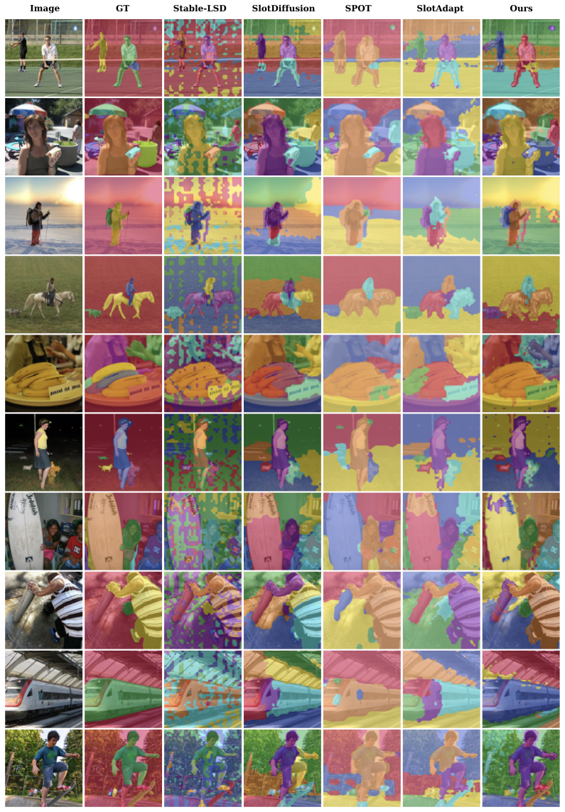
<figure id="appendix:fig:edited_samples" data-latex-placement="!htp">
<img src="/posts/2026/01/2026-01-03-190628-improved_object_centric_diffusion_learning_with_re/edited_samples.png" style="width:100%" /> style="width:95.0%" />
<figcaption>Illustration of compositional editing. <code>CODA</code> can
compose novel scenes from real-world images by removing (left) or
swapping (right) the slots, shown as masked regions in the
images.</figcaption>
</figure>
#### Ablation studies
<figure id="fig:ablation_example" data-latex-placement="!htp">
<img src="/posts/2026/01/2026-01-03-190628-improved_object_centric_diffusion_learning_with_re/examples_ablation.png" style="width:100%" /> />
<figcaption>Illustration of the ablation study on VOC. We start from the
pretrained diffusion model as a slot decoder (Baseline), adding register
slots (Reg), finetuning the key, value, and output projections in the
cross-attention layers (CA), adding contrastive alignment
(CO).</figcaption>
</figure>
We conduct ablations to evaluate the contribution of each component in
our framework, with results on the VOC dataset summarized in
<a href="#table:ablation_voc" data-reference-type="ref+label"
data-reference="table:ablation_voc">5</a>. The baseline (first row) uses
the frozen SD as a slot decoder. Finetuning the key, value, and output
projections of the cross-attention layers (**CA**) yields moderate
gains. Introducing register slots (**Reg**) provides substantial
improvements, particularly in mBO, by reducing slot entanglement. Adding
the contrastive loss (**CO**) further boosts mIoU; however, applying it
without stopping gradients in the diffusion model ($`\circ`$) degrades
performance. When combined, all components yield the best overall
results, as shown in the final row, with qualitative examples in
<a href="#fig:ablation_example" data-reference-type="ref+label"
data-reference="fig:ablation_example">4</a>. Further ablation studies on
the COCO dataset are reported
in <a href="#appendix:table:register_affect"
data-reference-type="ref+label"
data-reference="appendix:table:register_affect">3</a> and additional
results are provided in
<a href="#appendex:additional_results" data-reference-type="ref+label"
data-reference="appendex:additional_results">5</a>. Overall, the
ablations demonstrate that each component contributes complementary
benefits in enhancing compositional slot representations.
<figure id="table:ablation_voc" data-latex-placement="!htp">
<div class="minipage">
<img src="/posts/2026/01/2026-01-03-190628-improved_object_centric_diffusion_learning_with_re/segmentation_samples.png" style="width:100%" /> />
</div>
<div class="minipage">
<p><span id="table:ablation_voc"
data-label="table:ablation_voc"></span></p>
</div>
<figcaption>Segmentation masks learned by <code>CODA</code> on
COCO</figcaption>
</figure>
### Conclusions
We introduced `CODA`, a diffusion-based OCL framework that augments slot
sequences with input-independent register slots and a contrastive
alignment objective. Unlike prior approaches that rely solely on
denoising losses or architectural biases, `CODA` explicitly encourages
slot–image alignment, leading to stronger compositional generalization.
Importantly, it requires no architectural modifications or external
supervision, yet achieves strong performance across synthetic and
real-world benchmarks, including COCO and VOC. Despite its current
limitations
(<a href="#appedix:limitation" data-reference-type="ref+label"
data-reference="appedix:limitation">6</a>), these results highlight the
value of register slots and contrastive learning as powerful tools for
advancing OCL.
### Reproducibility Statement
<a href="#appedix:implementation_details"
data-reference-type="ref+label"
data-reference="appedix:implementation_details">2.4</a> provides
implementation details of `CODA` along with the hyperparameters used in
our experiments. All datasets used in this work are publicly available
and can be accessed through their official repositories. To ensure full
reproducibility, the source code is available as supplementary material.
### LLM Usage
In this work, large language models (LLMs) were used only to help with
proofreading and enhancing the clarity of the text. All research ideas,
theoretical developments, experiments, and implementation were conducted
entirely by the authors.
### Ethics Statement
This work focuses on improving OCL and compositional image generation
using pretrained diffusion models. While beneficial for controllable
visual understanding, it carries risks: (i) misuse, as compositional
generation could create misleading or harmful content; and (ii) bias
propagation, since pretrained diffusion models may reflect biases in
their training data, which can appear in generated images or
representations. Our method is intended for research on OCL and
representation, not for deployment in production systems without careful
considerations.
# Appendix
### Proofs
#### Proof of <a href="#the:mi" data-reference-type="ref+label"
data-reference="the:mi">1</a>
To prove <a href="#the:mi" data-reference-type="ref+label"
data-reference="the:mi">1</a>, we build on theoretical results that
connect data distributions with optimal denoising regression. Let define
the MMSE estimator of $`{\boldsymbol{\epsilon}}`$ from a noisy channel
$`{\mathbf{z}}_\gamma`$, which mixes $`{\mathbf{z}}`$ and
$`{\boldsymbol{\epsilon}}`$ at noise level $`\gamma`$ as
``` math
\begin{align*}
\hat{{\boldsymbol{\epsilon}}}({\mathbf{z}}_\gamma, \gamma)= \mathbb{E}_{{\boldsymbol{\epsilon}}\sim p({\boldsymbol{\epsilon}}\mid {\mathbf{z}}_\gamma)}[{\boldsymbol{\epsilon}}] = \underset{\tilde{{\boldsymbol{\epsilon}}}({\mathbf{z}}_\gamma, \gamma)}{ \arg \min} \,\, \mathbb{E}_{p({\boldsymbol{\epsilon}})p({\mathbf{z}})} \left[ \| {\boldsymbol{\epsilon}}- \tilde{{\boldsymbol{\epsilon}}}({\mathbf{z}}_\gamma, \gamma) \|_2^2\right] \,.
\end{align*}showed that the log-likelihood of $`{\mathbf{z}}`$ can be written solely in terms of the MMSE solution:
\begin{align}
    \log p({\mathbf{z}}) = -\frac{1}{2} \int_{-\infty}^{\infty} \mathbb{E}_{\boldsymbol{\epsilon}}\left[\| {\boldsymbol{\epsilon}}- \hat{{\boldsymbol{\epsilon}}}({\mathbf{z}}_\gamma, \gamma) \|^2 \right] d\gamma + c \,, \label{eq:nll_unconditional}
\end{align}where $`c = -\frac{D}{2} \log(2\pi e) + \frac{D}{2}\int_{-\infty}^\infty \sigma (\gamma) d\gamma`$ is a constant independent of the data, with $`D`$ denoting the dimensionality of $`{\mathbf{z}}`$.
Analogously, defining the optimal denoiser $`\hat{{\boldsymbol{\epsilon}}}({\mathbf{z}}_\gamma, \gamma, {\mathbf{s}})`$ for the conditional distribution $`p({\mathbf{z}}\mid {\mathbf{s}})`$ yields
\begin{align}
    \log p({\mathbf{z}}\mid {\mathbf{s}}) = -\frac{1}{2} \int_{-\infty}^{\infty} \mathbb{E}_{\boldsymbol{\epsilon}}\left[\| {\boldsymbol{\epsilon}}- \hat{{\boldsymbol{\epsilon}}}({\mathbf{z}}_\gamma, \gamma, {\mathbf{s}}) \|^2 \right] d\gamma + c \,. \label{eq:nll_conditional}
\end{align}Let $`\tilde{{\mathbf{s}}} \sim q(\tilde{{\mathbf{s}}} \mid {\mathbf{z}})`$ denote slots sampled from an auxiliary distribution $`q(\tilde{{\mathbf{s}}}\mid {\mathbf{z}})`$, which may differ from $`p(\tilde{{\mathbf{s}}} \mid {\mathbf{z}})`$. Using the KL divergence, we obtain
\begin{align*}
    D_{\mathrm{KL}}\left(q(\tilde{{\mathbf{s}}} \mid {\mathbf{z}}) || p(\tilde{{\mathbf{s}}} \mid {\mathbf{z}}) \right) &=  \mathbb{E}_{q(\tilde{{\mathbf{s}}}\mid {\mathbf{z}})} \left[ \log \frac{q(\tilde{{\mathbf{s}}}\mid {\mathbf{z}})}{ p(\tilde{{\mathbf{s}}} \mid {\mathbf{z}})} \right] \\
    &= \mathbb{E}_{q(\tilde{{\mathbf{s}}} \mid {\mathbf{z}})} \left[ \log q(\tilde{{\mathbf{s}}}\mid {\mathbf{z}}) - \log p({\mathbf{z}}\mid \tilde{{\mathbf{s}}}) - \log p(\tilde{{\mathbf{s}}}) + \log p({\mathbf{z}}) \right] \\
    &= -\mathbb{E}_{q(\tilde{{\mathbf{s}}}\mid {\mathbf{z}})} \left[\log p({\mathbf{z}}\mid \tilde{{\mathbf{s}}}) \right] + D_{\mathrm{KL}}(q(\tilde{{\mathbf{s}}}\mid {\mathbf{z}}) || p(\tilde{{\mathbf{s}}}))  + \log p({\mathbf{z}})\,.
\end{align*}This leads to the following decomposition of the marginal distribution:
\begin{align*}
    \log p({\mathbf{z}})  & = \mathbb{E}_{q(\tilde{{\mathbf{s}}}\mid {\mathbf{z}})} [\log p({\mathbf{z}}\mid \tilde{{\mathbf{s}}})] + D_{\mathrm{KL}}( q(\tilde{{\mathbf{s}}}\mid {\mathbf{z}}) || p(\tilde{{\mathbf{s}}} \mid {\mathbf{z}})) - D_{\mathrm{KL}}(q(\tilde{{\mathbf{s}}}\mid {\mathbf{z}}) || p(\tilde{{\mathbf{s}}}))
\end{align*}Consequently, the mutual information (MI) between $`{\mathbf{z}}`$ and $`{\mathbf{s}}`$ can be expressed as
\begin{align*}
    I({\mathbf{z}}; {\mathbf{s}}) &=  \mathbb{E}_{p({\mathbf{z}}, {\mathbf{s}})}\left[ \log p({\mathbf{z}}\mid {\mathbf{s}}) \right]  - \mathbb{E}_{p({\mathbf{z}})} \left[ \log p({\mathbf{z}}) \right] \\
    &= \mathbb{E}_{p({\mathbf{z}}, {\mathbf{s}})}\left[ \log p({\mathbf{z}}\mid {\mathbf{s}}) \right]  -  \mathbb{E}_{p({\mathbf{z}})}\mathbb{E}_{q(\tilde{{\mathbf{s}}} \mid {\mathbf{z}})} [\log p({\mathbf{z}}\mid \tilde{{\mathbf{s}}})] \\
    & \quad - \mathbb{E}_{p({\mathbf{z}})}[ D_{\mathrm{KL}}( q(\tilde{{\mathbf{s}}} \mid {\mathbf{z}}) || p(\tilde{{\mathbf{s}}} \mid {\mathbf{z}})) - D_{\mathrm{KL}}(q(\tilde{{\mathbf{s}}} \mid {\mathbf{z}}) || p(\tilde{{\mathbf{s}}}))]
\end{align*}From [eq:nll_conditional], it follows that
\begin{align}
  -I({\mathbf{z}}; {\mathbf{s}}) &=  \frac{1}{2}  \int_{-\infty}^{\infty}  \mathbb{E}_{({\mathbf{z}}, {\mathbf{s}}), {\boldsymbol{\epsilon}}} \left[\| {\boldsymbol{\epsilon}}- \hat{{\boldsymbol{\epsilon}}}({\mathbf{z}}_\gamma, \gamma, {\mathbf{s}}) \|^2 \right] d\gamma  - \frac{1}{2} \int_{-\infty}^{\infty} \mathbb{E}_{({\mathbf{z}}, \tilde{{\mathbf{s}}}), {\boldsymbol{\epsilon}}} \left[\| {\boldsymbol{\epsilon}}- \hat{{\boldsymbol{\epsilon}}}({\mathbf{z}}_\gamma, \gamma, \tilde{{\mathbf{s}}}) \|^2 \right] d\gamma \nonumber\\
  & \quad + \mathbb{E}_{{\mathbf{z}}}\left[ D_{\mathrm{KL}}( q(\tilde{{\mathbf{s}}}\mid {\mathbf{z}}) || p(\tilde{{\mathbf{s}}} \mid {\mathbf{z}})) - D_{\mathrm{KL}}(q(\tilde{{\mathbf{s}}} \mid {\mathbf{z}}) || p(\tilde{{\mathbf{s}}}))\right] \nonumber\\
  &= \frac{1}{2}  \int_{-\infty}^{\infty} \Big(\mathbb{E}_{({\mathbf{z}}, {\mathbf{s}}), {\boldsymbol{\epsilon}}} \left[\| {\boldsymbol{\epsilon}}- \hat{{\boldsymbol{\epsilon}}}({\mathbf{z}}_\gamma, \gamma, {\mathbf{s}}) \|^2 \right] - \mathbb{E}_{({\mathbf{z}}, \tilde{{\mathbf{s}}}), {\boldsymbol{\epsilon}}} \left[\| {\boldsymbol{\epsilon}}- \hat{{\boldsymbol{\epsilon}}}({\mathbf{z}}_\gamma, \gamma, \tilde{{\mathbf{s}}}) \|^2 \right] \Big)d\gamma \nonumber \\
  & \quad + \mathbb{E}_{{\mathbf{z}}}\left[ D_{\mathrm{KL}}( q(\tilde{{\mathbf{s}}}\mid {\mathbf{z}}) || p(\tilde{{\mathbf{s}}} \mid {\mathbf{z}})) - D_{\mathrm{KL}}(q(\tilde{{\mathbf{s}}} \mid {\mathbf{z}}) || p(\tilde{{\mathbf{s}}}))\right] \,, \label{eq:main_theorem}
\end{align}which completes the proof. $`\square`$
Proof of <a href="#coro:one" data-reference-type=“ref+label”
data-reference=“coro:one”>1
Under the assumption that $`q(\tilde{{\mathbf{s}}} \mid {\mathbf{z}}) = p(\tilde{{\mathbf{s}}})`$, it yields
\begin{align}
    \mathbb{E}_{{\mathbf{z}}} \left[ D_{\mathrm{KL}}(q(\tilde{{\mathbf{s}}} \mid {\mathbf{z}}) || p(\tilde{{\mathbf{s}}}))\right] &= \mathbb{E}_{{\mathbf{z}}} \left[ D_{\mathrm{KL}}(p(\tilde{{\mathbf{s}}}) || p(\tilde{{\mathbf{s}}}))\right] \nonumber \\
    &= 0 \, . \label{eq:second_kl}
\end{align}Similarly, the expected KL-divergence term in [eq:main_theorem] simplifies as follows:
\begin{align}
    \mathbb{E}_{{\mathbf{z}}}\left[ D_{\mathrm{KL}}( q(\tilde{{\mathbf{s}}}\mid {\mathbf{z}}) || p(\tilde{{\mathbf{s}}} \mid {\mathbf{z}})) \right] &= \mathbb{E}_{{\mathbf{z}}}\left[ D_{\mathrm{KL}}( p(\tilde{{\mathbf{s}}}) || p(\tilde{{\mathbf{s}}} \mid {\mathbf{z}})) \right] \nonumber \\
    &= \mathbb{E}_{p({\mathbf{z}})p(\tilde{{\mathbf{s}}})} \left[ \log \frac{p(\tilde{{\mathbf{s}}})}{p(\tilde{{\mathbf{s}}} \mid {\mathbf{z}})} \right] \nonumber \\
    &= \mathbb{E}_{p({\mathbf{z}})p(\tilde{{\mathbf{s}}})} \left[ \log \frac{p({\mathbf{z}}) p(\tilde{{\mathbf{s}}})}{p(\tilde{{\mathbf{s}}}, {\mathbf{z}})} \right] \nonumber \\
    &=  D_{\mathrm{KL}}(p({\mathbf{z}})p({\mathbf{s}}) || p({\mathbf{z}}, {\mathbf{s}})) \,.  \label{eq:first_kl}
\end{align}Substituting [eq:first_kl,eq:second_kl] into [eq:main_theorem] completes the proof. $`\square`$
Remark 1. [eq:first_kl] shows that the additional expected KL-divergence reduces to the reverse KL divergence between the product of marginals $`p({\mathbf{z}})p({\mathbf{s}})`$ and the joint distribution $`p({\mathbf{z}}, {\mathbf{s}})`$. This term complements the standard mutual information $`I({\mathbf{z}};{\mathbf{s}})`$, and together they form the Jeffreys divergence. Intuitively, while MI penalizes approximating the joint by the independent model, the reverse KL penalizes the opposite mismatch, thereby reinforcing the statistical dependence between $`{\mathbf{z}}`$ and $`{\mathbf{s}}`$.
Experimental setup
This section outlines the experimental setup of our study. We detail the datasets, baseline methods, evaluation metrics, and implementation choices used in all experiments.
Datasets
MOVi-C/E . These two variants of the MOVi benchmark are generated with the Kubric simulator. Following prior works , we evaluate on the 6,000-image validation set, since the official test sets are designed for out-of-distribution (OOD) evaluation. MOVi-C consists of complex objects and natural backgrounds, while MOVi-E includes scenes with a large numbers of objects (up to 23) per image.
VOC . We use the PASCAL VOC 2012 “trainaug” split, which includes 10,582 images: 1,464 images from the official train set and 9,118 images from the SDB dataset . This configuration is consistent with prior works . Training images are augmented with center cropping and then random horizontal flipping applied with a probability of 0.5. For evaluation, we use the official segmentation validation set of 1,449 images, where unlabeled pixels are excluded from scoring.
COCO . For experiments, we use the COCO 2017 dataset, consisting of 118,287 training images and 5,000 validation images. Training images are augmented with center cropping followed by random horizontal flipping with probability 0.5. For evaluation, we follow standard practice by excluding crowd instance annotations and ignoring pixels corresponding to overlapping objects.
Baselines
We compare CODA against state-of-the-art fully unsupervised OCL
models. The baselines include SA , DINOSAUR , SLATE , SLATE$`^+`$ (a
variant using a pretrained VQGAN instead of a dVAE), SPOT2 ,
Stable-LSD3 SlotDiffusion4 , and SlotAdapt . For DINOSAUR, we
evaluate both MLP and autoregressive Transformer decoders. For SPOT, we
report results with and without test-time permutation ensembling (SPOT
w/ ENS, SPOT w/o ENS). We use the pretrained checkpoints released by the
corresponding authors for SPOT and SlotDiffusion.
Metrics
Foreground Adjusted Rand Index (FG-ARI). The Adjusted Rand Index (ARI) measures the similarity between two partitions by counting pairs of pixels that are consistently grouped together (or apart) in both segmentations. The score is adjusted for chance, with values ranging from 0 (random grouping) to 1 (perfect agreement). The Foreground ARI (FG-ARI) is a variant that evaluates agreement only on foreground pixels, excluding background regions.
Mean Intersection over Union (mIoU). The Intersection over Union (IoU) between a predicted segmentation mask and its ground-truth counterpart is defined as the ratio of their intersection to their union. The mean IoU (mIoU) is obtained by averaging these IoU values across all objects and images in the dataset. This metric measures how well the predicted segmentation masks overlap with the ground-truth masks, aggregated over all instances.
Mean Best Overlap (mBO). The Best Overlap (BO) score for a predicted segmentation mask is defined as the maximum IoU between that predicted mask and any ground-truth object mask in the image. The mean BO (mBO) is then computed by averaging these BO scores across all predicted masks in the dataset. Unlike mIoU, which evaluates alignment with ground-truth objects directly, mBO emphasizes how well each predicted mask corresponds to its best-matching object, making it less sensitive to under- or over-segmentation.
Implementation details
The hyperparameters are summarized in
1. We initialize the U-Net denoiser
and VAE components from Stable Diffusion v1.55 . During training,
only the key, value, and output projections in the cross-attention
layers are finetuned, while all other components remain frozen. For slot
extraction, we employ DINOv26 with a ViT-B backbone and a patch size
of 14, producing feature maps of size $`32\times32`$. The input
resolution is set to $`512\times512`$ for the diffusion model and
$`448\times448`$ for SA. As a form of data augmentation, we apply random
horizontal flipping (Rand.HFlip) during training with a probability of
0.5. The negative slots are constructed by replacing 50% of the original
slots with a subset of slots sampled from other images within the batch.
CODA is trained using the Adam optimizer with a learning rate of
$`2 \times 10^{-5}`$, a weight decay of $`0.01`$, and a constant
learning rate schedule with a warm-up of 2500 steps. To improve
efficiency and stability, we use 16-bit mixed precision and gradient
norm clipping at 1. All models are trained on 4 NVIDIA A100 GPUs with a
local batch size of 32. We train for 500k steps on the COCO dataset and
250k steps on all other datasets. Training takes approximately 5.5 days
for COCO and 2.7 days for the remaining datasets. For evaluation, the
results are averaged over five random seeds. To ensure a fair
comparision, for all FID and KID evaluations, we downsample CODA’s
$`512\times512`$ outputs to $`256\times256`$, matching the resolution
used in prior works.
Attention masks for evaluation. We evaluate object segmentation using the attention masks produced by SA. At each slot iteration, attention scores are first computed using the standard $`\mathtt{softmax}`$ along the slot axis and then normalized via a weighted mean:
\begin{align*}
    {\mathbf{m}}^{(t)} = \underset{N}{\mathtt{softmax}} \left( \frac{q({\mathbf{s}}^{(t)}) k({\mathbf{f}})^\top}{\sqrt{D}} \right)  \Longrightarrow \quad {\mathbf{m}}^{(t)}_{m,n} = \frac{{\mathbf{m}}^{(t)}_{m,n}}{\sum_{l=1}^M {\mathbf{m}}^{(t)}_{l,n}} \,,
\end{align*}where $`D`$ denotes the dimension of $`k({\mathbf{f}})`$. The soft attention masks from the final iteration are converted to hard masks with $`\mathtt{arg max}`$ and used as the predicted segmentation masks for evaluation. This procedure ensures that each pixel is assigned to the slot receiving the highest attention weight.
| Hyperparameter | MOVi-C | MOVi-E | VOC | COCO |
|---|---|---|---|---|
| General | ||||
| Training steps | 250k | 250k | 250k | 500k |
| Learning rate | $`2\times 10^{-5}`$ | $`2\times 10^{-5}`$ | $`2\times 10^{-5}`$ | $`2\times 10^{-5}`$ |
| Batch size | 32 | 32 | 32 | 32 |
| Learning rate warm up | 2500 | 2500 | 2500 | 2500 |
| Optimizer | AdamW | AdamW | AdamW | AdamW |
| ViT architecture | DINOv2 ViT-B | DINOv2 ViT-B | DINOv2 ViT-B | DINOv2 ViT-B |
| Diffusion | SD v.1.5 | SD v.1.5 | SD v.1.5 | SD v.1.5 |
| Gradient norm clipping | 1 | 1 | 1 | 1 |
| Weighting $`\lambda_{\mathrm{cl}}`$ | 0.05 | 0.05 | 0.05 | 0.03 |
| Image specification | ||||
| Image size | 512 | 512 | 512 | 512 |
| Augmentation | Rand.HFlip | Rand.HFlip | Rand.HFlip | Rand.HFlip |
| Crop | Full | Full | Central | Central |
| Slot attention | ||||
| Input resolution | $`32 \times 32`$ | $`32 \times 32`$ | $`32 \times 32`$ | $`32 \times 32`$ |
| Number of slots | 11 | 24 | 6 | 7 |
| Number of iterations | 3 | 3 | 3 | 3 |
| Slot size | 768 | 768 | 768 | 768 |
Hyperparameters used for CODA on MOVi-C, MOVi-E, VOC, and COCO
datasets
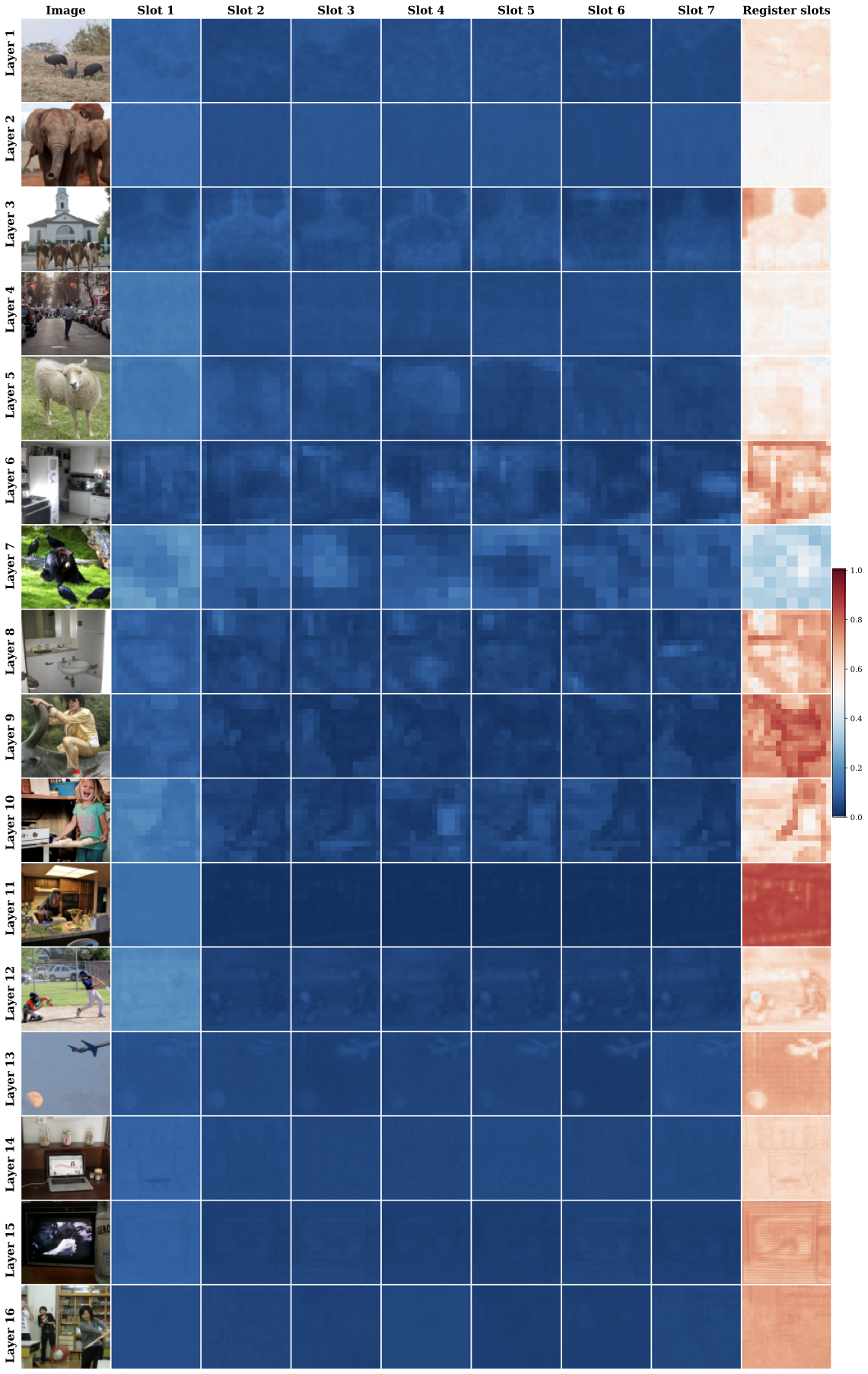
Visualization of attention scores
We visualize the attention scores in
6, showing the
average attention mass assigned to semantic slots versus register slots.
CODA is trained on the COCO dataset, and illustrative images are
randomly sampled. Since the cross-attention layers in SD are multi-head,
we average the attention maps across both heads and noise levels.
Interestingly, although register slots are semantically empty, they consistently absorb a substantial portion of the attention mass. This arises from the $`\mathtt{softmax}`$ normalization, which forces attention scores to sum to one across all slots. When a query does not strongly correspond to any semantic slot, the model must still allocate its attention; register slots act as neutral sinks that capture these residual values. This mechanism helps preserve clean associations between semantic slots and object concepts.
 style="width:97.0%" />
CODA. Each image in row
Layer i and
column Slot j
visualizes the total attention mass assigned to slot j at layer i. The last column reports the total
attention mass absorbed by the register slots. CODA
heavily attends to the register slots across all
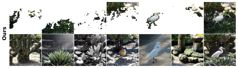
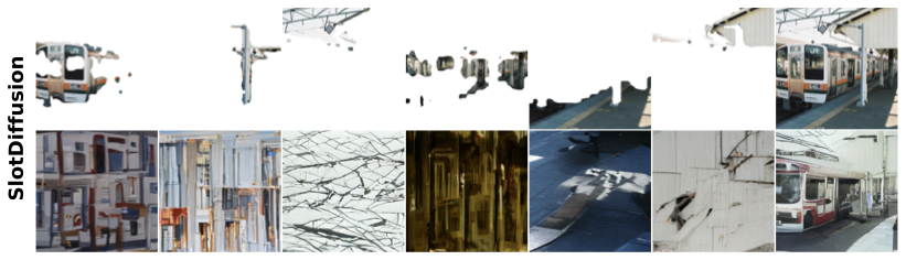
layers.Compositional image generation from individual slots
We evaluate the ability of diffusion-based OCL methods to generate
images from individual slots. As shown in
7, each input image is
decomposed into six slots, with each slot intended to represent a
distinct concept. We then condition the decoder on individual slots to
generate single-concept images. The last column shows reconstructions
using all slots combined. While all methods can reconstruct the original
images when conditioned on the full slot set, most fail to produce
faithful generations from individual slots. Specifically, Stable-LSD
produces mostly texture-like patterns that poorly match the intended
concepts, while SlotDiffusion , despite being trained end-to-end, also
struggles to generate coherent objects. In Stable-LSD, slots are jointly
trained to reconstruct the full scene, so object information can be
distributed across multiple slots rather than concentrated in any single
one. Consequently, removing all but one slot at test time puts the model
in an out-of-distribution regime, and single-slot generations do not
yield coherent objects even though the full slot set reconstructs the
image well. This reflects slot entanglement where individual slots mix
features from multiple objects. SlotAdapt partially alleviates this
issue through an average register token, but since their embedding is
injected directly into the cross-attention layers and tied to
input-specific features, it limits flexibility in reusing slots across
arbitrary compositions. In contrast, the input-independent register
slots introduced in CODA act as residual sinks and do not encode
input-specific features, enabling more faithful single-slot generations
and greater compositional flexibility.
To quantify these results, we report FID and KID scores by comparing
single-slot generations against the real images in the training set. For
each validation image, we extract six slots and generate six
corresponding single-slot images, ensuring a fair comparison across
methods. Results on the VOC dataset are reported in
4, where CODA
achieves the best scores, confirming its ability to generate coherent
and semantically faithful images from individual slots.
Although register slots substantially reduce background entanglement, they do not enforce a hard separation between foreground and background. The attention mechanism in SA still remains soft, and our objectives do not explicitly prevent semantic slots from attending to background regions. As a result, semantic slots may still absorb contextual pixels, especially near object boundaries or in textured areas that are useful for reconstruction, when the number of slots exceeds the number of objects. As a result, small “meaningless” background fragments may still be assigned to semantic slots, as seen in 7. Empirically, however, we find that register slots substantially decrease background leakage compared to baselines without registers.
 style="width:90.0%" />
style="width:90.0%" />
style="width:90.0%" />
style="width:90.0%" />
style="width:90.0%" />
style="width:90.0%" />
style="width:90.0%" />
CODA, register slots can be regarded as part of the U-Net
architecture as they are independent from the input. Compared to
baselines, our method generates faithful images from individual
slots.Additional results
In this section, we present supplementary quantitative and qualitative
results that provide further insights into the performance of CODA.
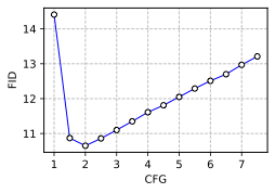
Classifier-free guidance
To enhance image generation quality, we employ classifier-free guidance
(CFG) , which interpolates between conditional and unconditional
diffusion predictions. A guidance scale of $`\mathrm{CFG}=1`$
corresponds to standard conditional generation. We conduct an ablation
study on different CFG values to assess their impact on generation
quality. As shown in
8, both FID and KID scores
improve with moderate guidance, with CODA achieving the best
performance at $`\mathrm{CFG}=2.0`$. This indicates that a balanced
level of guidance enhances fidelity without over-amplifying artifacts.
 style="width:35.0%" />
 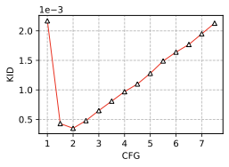 style="width:35.0%" />
Learnable register slots
Several works have explored trainable tokens as auxiliary inputs to
transformers. For example, the [CLS] token is commonly introduced for
classification in ViT and BERT , while CLIP employs an [EOS] token.
These tokens serve as learnable registers that allow the model to store
and retrieve intermediate information during inference. demonstrated
that appending such tokens can boost performance by increasing token
interactions, thereby promoting deeper computation. Similarly, utilized
register tokens during pretraining to mitigate the emergence of
high-norm artifacts. Motivated by these findings, we experiment with
replacing our frozen CLIP-derived register slots with learnable ones.
These slots are appended to the slot sequence but remain context-free
placeholders.
Results on VOC with varying numbers of learnable register slots are
shown in 2. The model
without register slots ($`R=0`$) performs the worst across all metrics
(FG-ARI, mBO$`^i`$, mBO$`^c`$, mIoU$`^i`$, and mIoU$`^c`$).
Interestingly, introducing just a single register slot leads to a
significant performance boost. Further increasing the number of tokens
to $`R=77`$, matching the configuration used in CODA, yields only
marginal improvements. Although more register slots could slightly
increase computational cost, this is negligible as the number of
register slots is relatively small. For instance, using 77 register
slots increases GPU time by only 0.02% compared to the baseline without
using any register slot. Interestingly, CODA achieves the best
performance when using frozen register slots. These findings emphasize
the effectiveness of register slots in improving the model performance.
| $`R`$ | FG-ARI$`\uparrow`$ | mBO$`^i`$$`\uparrow`$ | mBO$`^c`$$`\uparrow`$ | mIoU$`^i`$$`\uparrow`$ | mIoU$`^c`$$`\uparrow`$ |
|---|---|---|---|---|---|
| 0 | 15.44 | 47.03 | 52.63 | 49.75 | 55.63 |
| 1 | 30.39 | 54.47 | 59.96 | 50.21 | 55.34 |
| 4 | 29.89 | 54.91 | 60.15 | 50.65 | 55.65 |
| 64 | 30.40 | 54.62 | 59.93 | 50.47 | 55.45 |
| 77 | 30.21 | 55.26 | 60.89 | 50.86 | 56.07 |
CODA |
32.23 | 55.38 | 61.32 | 50.77 | 56.30 |
Ablation study on varying the number of register slots on the VOC dataset
Additional ablation on COCO
We further examine the contribution of frozen register slots on the COCO dataset, using pretrained SD as the slot decoder baseline. Different settings are evaluated: (i) adding register slots (+Reg), (ii) adding register slots combined with finetuning the key, value, and output projections in cross-attention layers (+CA), and adding the contrastive loss (+CO). As shown in 3, register slots consistently improve performance in both cases, demonstrating their robustness and effectiveness when integrated into the slot sequence.
| Method | FG-ARI$`\uparrow`$ | mBO$`^i`$$`\uparrow`$ | mBO$`^c`$$`\uparrow`$ | mIoU$`^i`$$`\uparrow`$ | mIoU$`^c`$$`\uparrow`$ |
|---|---|---|---|---|---|
| Baseline | 20.99 | 29.77 | 37.21 | 32.16 | 41.25 |
| Baseline + Reg | 23.64 | 31.14 | 39.07 | 32.64 | 41.91 |
| Baseline + CA | 36.99 | 33.82 | 38.08 | 35.04 | 41.24 |
| Baseline + CA + Reg | 45.95 | 35.80 | 40.32 | 35.76 | 41.75 |
| Baseline + CO | 25.24 | 30.14 | 38.77 | 32.83 | 42.99 |
| Baseline + CO + CA | 35.84 | 34.36 | 38.67 | 36.28 | 42.85 |
Baseline + CA + Reg + CO (CODA) |
47.54 | 36.61 | 41.43 | 36.41 | 42.64 |
Ablation study on the COCO dataset
We further analyze the effect of the contrastive loss on image generation. Results are reported in 4. Without the contrastive loss, Reg+CA achieves slightly better FID/KID under compositional generation than the full model Reg+CA+CO. This aligns with the role of CO, which is primarily intended to strengthen slot–image alignment and object-centric representations rather than to maximize image fidelity, and can therefore marginally degrade FID/KID. Overall, CO should be viewed as an optional component that further improve object discovery at a small cost in visual quality.
| Metric | Reconstruction | Compositional generation | |||
|---|---|---|---|---|---|
| 2-3 | Reg + CA | Reg + CA + CO | Reg + CA | Reg + CA + CO | |
| KID×103 | 0.39 | 0.35 | 27.95 | 30.44 | |
| FID | 10.65 | 10.65 | 29.34 | 31.03 | |
Effect of the contrastive loss weighting
We conduct an ablation study to analyze the impact of the weighting coefficient $`\lambda_\mathrm{cl}`$ in the contrastive loss term of our objective function in [eq:total_loss]. Results on the COCO dataset are shown in 5. The study reveals that moderate values of $`\lambda_\mathrm{cl}`$ achieve the best trade-off between the denoising and contrastive objectives, yielding the strongest overall performance. In practice, very small weights underuse the contrastive signal, while excessively large weights destabilize training and harm reconstruction quality. Although the contrastive loss shares a similar form with the diffusion loss, in practice, we find that it needs to be weighted by a relatively small factor $`\lambda_\mathrm{cl}`$ to obtain good results. Empirically, increasing $`\lambda_\mathrm{cl}`$ consistently degrades visual quality. We hypothesize that this happens because the contrastive term operates on slot-level features and, when heavily weighted, over-emphasizes alignment at the expense of the diffusion prior, leading to overspecialized and less realistic samples. In contrast, a small $`\lambda_\mathrm{cl}`$ acts as a weak regularizer that improves alignment while keeping the diffusion objective dominant.
| $`\lambda_{\mathrm{cl}}`$ | FG-ARI$`\uparrow`$ | mBO$`^i`$$`\uparrow`$ | mBO$`^c`$$`\uparrow`$ | mIoU$`^i`$$`\uparrow`$ | mIoU$`^c`$$`\uparrow`$ |
|---|---|---|---|---|---|
| 0 | 45.95 | 35.80 | 40.32 | 35.76 | 41.75 |
| 0.001 | 46.07 | 35.99 | 40.50 | 36.18 | 42.18 |
| 0.002 | 45.93 | 35.88 | 40.79 | 35.74 | 42.02 |
| 0.003 | 47.54 | 36.61 | 41.43 | 36.41 | 42.60 |
| 0.004 | 46.87 | 36.38 | 41.13 | 36.26 | 42.41 |
| 0.005 | 44.98 | 35.80 | 40.86 | 35.44 | 41.75 |
Ablation study on varying the weighting terms in contrastive loss on the COCO dataset
Combination ratios for negative slots
This section explores different combination ratios for constructing
negative slots $`\tilde{{\mathbf{s}}}`$. As outlined
in 4.3, given two slot
sequences $`{\mathbf{s}}`$ and $`{\mathbf{s}}'`$ from two distinct
images $`{\mathbf{x}}`$ and $`{\mathbf{x}}'`$, we randomly replace a
fraction $`r \in (0,1]`$ of slots from $`{\mathbf{s}}`$ with those from
$`{\mathbf{s}}'`$. When $`r=1`$, the entire set of slots
$`{\mathbf{s}}`$ is replaced by $`{\mathbf{s}}'`$, while values
$`0
| $`r`$ | FG-ARI$`\uparrow`$ | mBO$`^i`$$`\uparrow`$ | mBO$`^c`$$`\uparrow`$ | mIoU$`^i`$$`\uparrow`$ | mIoU$`^c`$$`\uparrow`$ |
|---|---|---|---|---|---|
| 0.25 | 32.34 | 54.58 | 60.52 | 50.44 | 55.97 |
| 0.50 | 32.23 | 55.38 | 61.32 | 50.77 | 56.30 |
| 0.75 | 33.34 | 55.06 | 60.98 | 50.12 | 55.61 |
| 1.00 | 32.67 | 54.60 | 59.84 | 49.73 | 54.64 |
Ablation study on varying the portion of negative slots on the VOC dataset
Comparison with weakly-supervised baselines
We compare CODA to GLASS , a weakly supervised approach that uses a
guidance module to produce semantic masks as pseudo ground truth. In
particular, BLIP-2 is used for caption generation to create guidance
signals. While this supervision helps GLASS mitigate over-segmentation,
it also limits its applicability in fully unsupervised settings. In
contrast, CODA does not rely on any external supervision and can
distinguish between multiple instances of the same class, enabling more
fine-grained object separation and richer compositional editing.
[appendix:tab:glass] reports the
results. We additionally consider GLASS$`^\dagger`$, a variant of GLASS
that uses ground-truth class labels associated with the input image.
While GLASS achieves stronger performance on semantic segmentation
masks, it underperforms CODA on object discovery, as reflected by
lower FG-ARI scores. This suggests that CODA is better at
disentangling distinct object instances at a conceptual level.
Qualitative comparison
To complement the quantitative results in the main paper, we present
additional qualitative examples that illustrate the effectiveness of
CODA. These examples provide a more complete picture of the model’s
performance and highlight its advantages over previous approaches.
Object segmentation. We visualize segmentation results in
9. CODA
consistently discovers objects and identifies semantically meaningful
regions in a fully unsupervised manner. Compared to diffusion-based OCL
baselines such as Stable-LSD and SlotDiffusion, CODA produces cleaner
masks with fewer fragmented segments, leading to more coherent object
boundaries.
 />
/>
Reconstruction. [fig:appendix:visual_reconstruction:real_world,fig:appendix:visual_reconstruction:synthetic]
show reconstructed images generated by CODA. The results demonstrate
that CODA produces high-quality reconstructions when conditioned on
the learned slots. Importantly, the generated images preserve semantic
consistency while exhibiting visual diversity, indicating that the slots
capture abstract and meaningful representations of the objects in the
scene.
Compositional generation.
12 showcases COCO image edits
based on CODA’s learned slots, including object removal, replacement,
addition, and background modification. We find that the editing
operations are highly successful, introducing only minor adjustments
while consistently preserving high image quality.
CODA.CODA.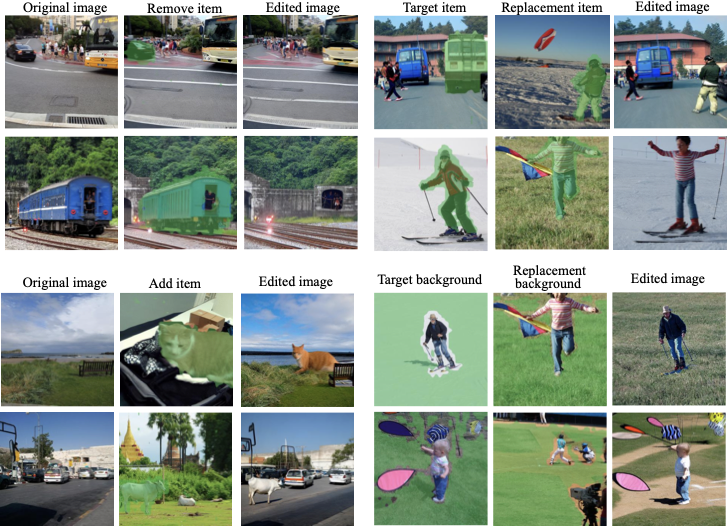 />
/>
CODA composes novel scenes from real-world images by
removing (top left), swapping (top right), and adding (bottom left)
slots, as well as changing the background (bottom right). The masked
objects indicate the slots that are added, removed, or replaced relative
to the original image.Limitations and future work
While CODA achieves strong performance across synthetic and real-world
benchmarks, it has several limitations that open avenues for future
research. (i) CODA relies on DINOv2 features and SD backbones, which
may inherit dataset-specific biases and limit generalization to domains
with very different visual statistics. (ii) While our contrastive loss
improves slot–image alignment, full disentanglement in cluttered or
ambiguous scenes remains an open challenge. (iii) Inherited from SA,
CODA still requires the number of slots to be specified in advance.
This restricts flexibility in scenes with a variable or unknown number
of objects, and can lead to either unused slots or missed objects . In
our implementation, CODA uses a fixed number of semantic slots plus a
small number of register slots. Note that the register slots do not
reduce semantic capacity but also cannot resolve the fundamental
bottleneck when the true number of objects exceeds the available
semantic slots, in which case objects may still be merged into the same
slot despite reduced background entanglement. This is because the
contrastive alignment is defined only for semantic slots, which
encourages them to explain object-level content, while register slots
are discouraged from encoding object-like structure.
Despite our improvements in object discovery and compositional control, faithfully preserving fine-grained images in reconstructions and compositional edits remains challenging, as also observed in prior slot diffusion models (e.g., SlotAdapt). We attribute this to several factors: (i) slot representations act as a low-dimensional bottleneck that must compress both geometry and detailed appearance; (ii) the diffusion backbone is pretrained to model images (and text–image pairs) but not to decode from slot-based object latents; and (iii) our training objective emphasizes object-centric grouping and controllability rather than exact pixel-level reconstruction. Improving image reconstruction in OCL is an important direction for future work.
Although CODA is conceptually compatible with a wide range of diffusion
backbones, in this work we restrict ourselves to a relatively small,
widely used backbone to ensure fair comparison with prior object-centric
methods (e.g., SlotAdapt, LSD) and to keep computational and memory
requirements manageable. We do not explore scaling CODA to larger, more
recent architectures such as SDXL or FLUX , which would require
substantially more resources and additional engineering effort to handle
larger feature maps, model sizes, and more sophisticated
text-conditioning pipelines (e.g., multiple text encoders and auxiliary
pooled text embeddings). Despite these limitations, we believe that
CODA offers a scalable and conceptually simple foundation for
advancing OCL. A promising direction for future work is extending CODA
to Diffusion Transformers (DiTs) , where slot representations could
naturally replace or complement text embeddings in cross-attention,
enabling richer and more flexible compositional control, as well as
investigating integrations with larger backbones such as SDXL/FLUX to
more fully assess the generality of our approach.
📊 논문 시각자료 (Figures)

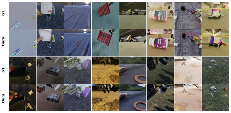
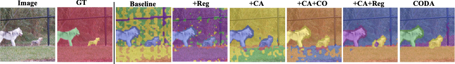
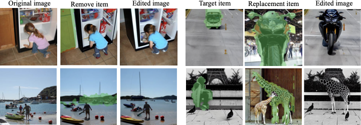
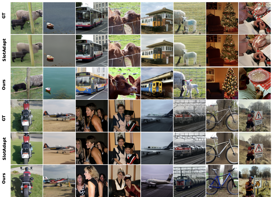
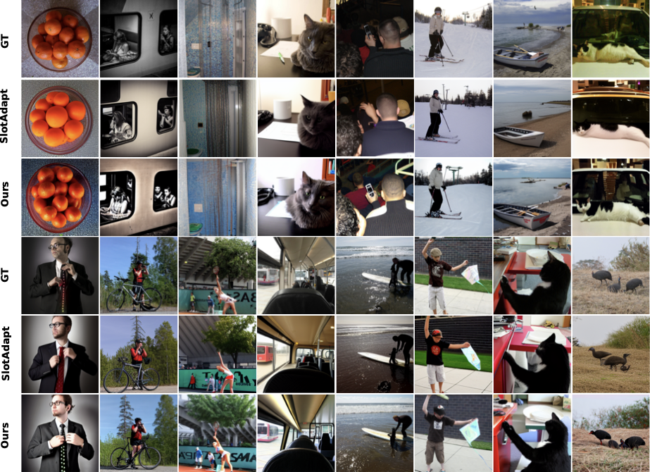
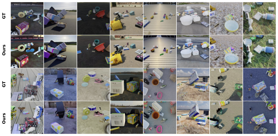
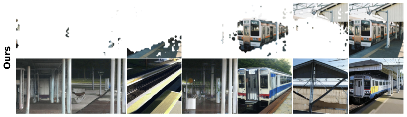
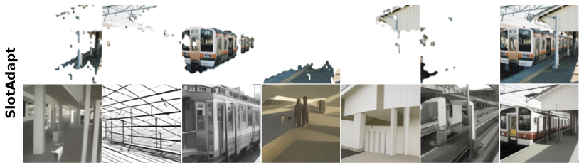
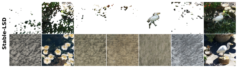
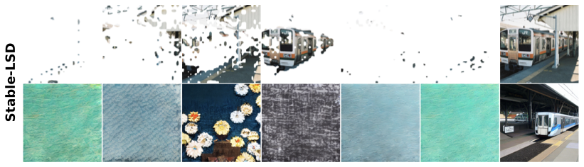
A Note of Gratitude
The copyright of this content belongs to the respective researchers. We deeply appreciate their hard work and contribution to the advancement of human civilization.-
For SD v1.5, 77 padding tokens are used, resulting in 77 register slots. ↩︎
-
https://huggingface.co/stable-diffusion-v1-5/stable-diffusion-v1-5 ↩︎