LLM Collusion
📝 Original Paper Info
- Title: LLM Collusion- ArXiv ID: 2601.01279
- Date: 2026-01-03
- Authors: Shengyu Cao, Ming Hu
📝 Abstract
We study how delegating pricing to large language models (LLMs) can facilitate collusion in a duopoly when both sellers rely on the same pre-trained model. The LLM is characterized by (i) a propensity parameter capturing its internal bias toward high-price recommendations and (ii) an output-fidelity parameter measuring how tightly outputs track that bias; the propensity evolves through retraining. We show that configuring LLMs for robustness and reproducibility can induce collusion via a phase transition: there exists a critical output-fidelity threshold that pins down long-run behavior. Below it, competitive pricing is the unique long-run outcome. Above it, the system is bistable, with competitive and collusive pricing both locally stable and the realized outcome determined by the model's initial preference. The collusive regime resembles tacit collusion: prices are elevated on average, yet occasional low-price recommendations provide plausible deniability. With perfect fidelity, full collusion emerges from any interior initial condition. For finite training batches of size $b$, infrequent retraining (driven by computational costs) further amplifies collusion: conditional on starting in the collusive basin, the probability of collusion approaches one as $b$ grows, since larger batches dampen stochastic fluctuations that might otherwise tip the system toward competition. The indeterminacy region shrinks at rate $O(1/\sqrt{b})$.💡 Summary & Analysis
1. **First Contribution**: Understanding how algorithms can lead to illegal collusion by comparing LLMs with reinforcement learning. 2. **Second Contribution**: Analyzing how shared algorithmic infrastructure and data sharing policies increase collusion risk. 3. **Third Contribution**: Theoretical framework that shows collusion can emerge as an unintended consequence of standard operational practices.📄 Full Paper Content (ArXiv Source)
The rapid adoption of algorithms in commercial decision-making has attracted increasing regulatory scrutiny. In March 2024, the Federal Trade Commission (FTC) and the Department of Justice (DOJ) issued a joint statement warning that algorithmic pricing systems can facilitate illegal collusion, even in the absence of explicit agreements among competitors.1 Subsequent enforcement signals have only intensified: in August 2025, DOJ Assistant Attorney General Gail Slater announced that algorithmic pricing investigations would significantly increase as deployment of the technology becomes more prevalent.2
This regulatory concern is particularly salient as sellers increasingly rely on large language models (LLMs) for pricing decisions, an area the regulation has not yet addressed. A 2024 McKinsey survey of Fortune 500 retail executives found that 90% have begun experimenting with generative AI solutions, with pricing and promotion optimization emerging as a priority use case.3 In Europe, 55% of retailers plan to pilot generative AI-based dynamic pricing by 2025, building on the 61% who have already adopted some form of algorithmic pricing.4 Industry applications are already operational: report that Alibaba has deployed an LLM-based pricing system on its Xianyu platform to provide real-time price recommendations for sellers.
This heightened regulatory pressure coincides with remarkable market concentration in the LLM industry. As of 2025, ChatGPT commands approximately 62.5% of the business-to-consumer AI subscription market, while 92% of Fortune 500 companies report using OpenAI products.5 This confluence of concentrated AI infrastructure and heightened antitrust concern raises a fundamental question: Can the widespread adoption of LLMs for pricing decisions facilitate collusion across competing sellers?
The possibility that algorithms might learn to collude has been studied extensively in the context of machine learning/reinforcement learning (RL). demonstrate that Q-learning agents can converge to supracompetitive prices in repeated games through trial-and-error learning. However, such collusion typically requires extensive training periods and millions of interactions, providing some reassurance that computational barriers might limit practical concern. LLMs present a fundamentally different paradigm. Unlike RL agents that learn pricing strategies from scratch through repeated market interactions, LLMs arrive pretrained on vast corpora of human knowledge, including business strategy, economic theory, and pricing practices. Recent experimental work by documents that LLM-based pricing agents converge to supracompetitive prices much more rapidly than their RL counterparts: GPT-4 agents reach near-optimal collusive pricing within 100 periods, compared to the hundreds of thousands to millions of periods required for Q-learning algorithms. Yet the theoretical mechanisms underlying this acceleration remain poorly understood.
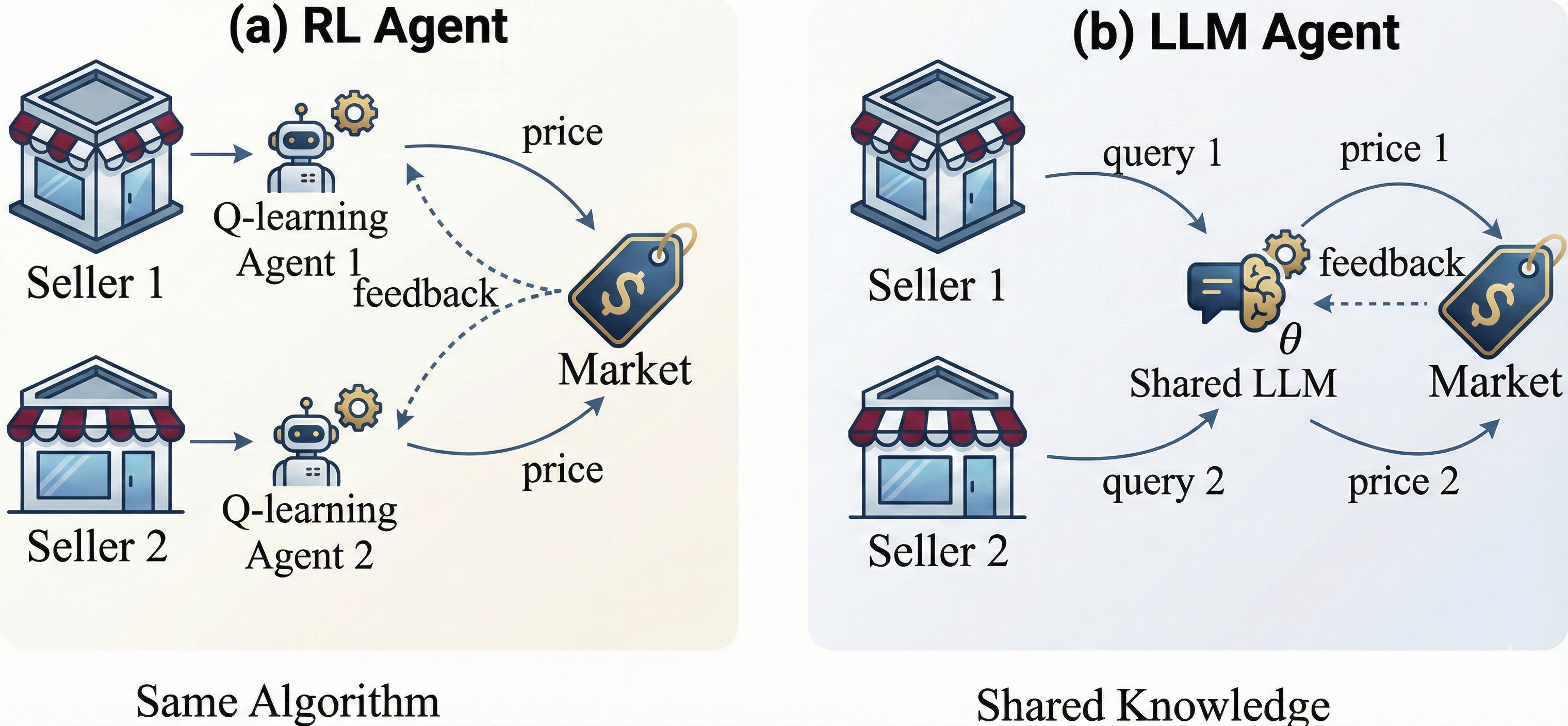
We identify two sources of collusion risk unique to LLM-based decision-making and illustrate the contrast between LLM-based and RL-based approaches in Figure 1. Specifically, the first source is the shared knowledge infrastructure that arises from market concentration. Given the dominant position documented above, competing sellers frequently delegate pricing decisions to the same LLM provider. When multiple sellers query the same model, their adopted recommendations may become correlated through the model’s internal latent preferences, a structural tendency toward certain pricing strategies encoded in its weights. This correlation creates implicit coordination without any communication between sellers: even if each seller queries the LLM independently, the common underlying preference induces positive correlation in their pricing actions. Moreover, shared knowledge persists even when sellers use different LLM providers. Leading LLMs are often distilled into smaller models by competitors, transferring embedded pricing heuristics from dominant providers to the broader ecosystem.6 In addition, pretraining corpora across providers draw from largely overlapping public sources, including business literature, economic textbooks, and strategic discussions that extensively document the profitability of coordinated pricing. Alignment procedures such as reinforcement learning from human feedback (RLHF) further homogenize model behavior, as evaluators or users at different companies apply similar standards of “helpfulness” and “reasonableness.” This raises a fundamental question: Does shared knowledge infrastructure, whether through common providers or homogenized training, lead to correlated pricing recommendations that translate into market-level collusion?
The second source of risk is the data sharing policies that govern model improvement. Major LLM providers collect user interaction data to refine their models, creating feedback loops between seller behavior and model updates. Google’s Gemini, for instance, uses a “Keep Activity” setting that is enabled by default for users aged 18 and over, allowing the platform to analyze conversations and use uploaded files, images, and videos for AI training.7 Anthropic’s August 2025 policy change similarly made data sharing the default setting, with five-year retention for users who consent.8 xAI offers $150 in monthly API credits to developers who share their interaction data, with no mechanism to opt out once the program is joined.9 When multiple sellers share their pricing interactions and outcomes with the same LLM provider, the model’s retraining process aggregates this data. A model that observes high prices leading to high profits across multiple sellers may update its preferences accordingly. This raises another fundamental question: Does data aggregation from competing sellers create a self-reinforcing feedback loop that drives prices toward collusive levels?
This paper develops a theoretical framework to analyze the emergence of collusion when sellers delegate pricing decisions to the same LLM, addressing these two questions. Surprisingly, we find that collusion can emerge as an unintended consequence of standard operational practices. In high-stakes tasks such as pricing, decision-makers typically configure LLMs for robustness and reproducibility by setting decoding temperatures to zero or near-zero. This seemingly prudent choice increases the correlation between the model’s internal preference and its generated outputs, thereby facilitating coordination without explicit communication. Moreover, infrequent retraining schedules necessitated by prohibitively high computational costs further amplify the risk of collusion. Major LLM providers typically release model updates every 6–12 months, translating into large effective batch sizes that suppress the beneficial noise which might otherwise allow prices to escape to competitive levels.
Model.
We consider a symmetric duopoly pricing game in which two sellers compete by simultaneously choosing between a high-price strategy ($`H`$) and a low-price strategy ($`L`$). Both sellers delegate their pricing decisions to the same LLM. The LLM’s behavior is characterized by two parameters: a propensity parameter $`\theta \in [0,1]`$ representing the model’s internal preference for high-price recommendations, and an output fidelity $`\rho \in [0.5,1]`$ capturing the alignment probability between this preference and the generated output. The LLM updates its propensity through model retraining: after observing actions and outcomes over every batch of $`b \geq 1`$ decision rounds, the model evaluates the relative performance of high-price versus low-price recommendations and adjusts $`\theta`$ accordingly. This update follows a log-odds recursion that increases $`\theta`$ when high prices outperform and decreases it otherwise.
Results.
We first analyze a benchmark setting in which the LLM retraining is performed on large batches of interaction data, so that estimation noise becomes negligible. We show that whether high-price recommendations become self-reinforcing depends on two competing forces: the benefit of coordination when both sellers receive and follow the same high-price recommendation, versus the cost of miscoordination when sellers receive different recommendations and the low-price seller captures the market. When output fidelity is sufficiently high, coordination benefits dominate, and learning reinforces the LLM’s preference for high prices.
It is worth noting that high output fidelity is precisely what decision-makers seek in practice. Low fidelity, corresponding to high-temperature decoding, introduces randomness into recommendations. Such unpredictability imposes operational costs on sellers: inconsistent pricing confuses customers and erodes brand equity, noisy outputs obscure whether realized profits stem from sound strategy or mere chance, and stochastic recommendations undermine the explainability that regulators increasingly demand of algorithmic pricing systems. Consequently, sellers naturally configure LLMs for robustness and reproducibility by setting decoding temperatures to zero or near-zero, which pushes output fidelity to high levels.
We establish a phase transition in long-run pricing behavior, governed by a critical output-fidelity threshold. Below this threshold, competitive pricing is the unique stable outcome: the LLM converges to recommending low prices regardless of its initial preference. Above this threshold, two stable outcomes coexist: competitive pricing and collusive pricing. Which outcome is realized depends on the model’s initial preference. When output fidelity is perfect, meaning the LLM’s recommendations perfectly reflect its internal preference, the system converges to full collusion from any interior starting point. The standard practice of configuring LLMs for reliability thus inadvertently pushes sellers into the parameter region where collusion can emerge.
We then analyze a more realistic setting in which the LLM is retrained on finite batches, so that randomness persists throughout learning. We show that the system still converges to a stable outcome, but which outcome is reached now depends on the random training data encountered along the way. Identical models with identical initial conditions can reach different long-run outcomes. We characterize how the probability of collusion depends on batch size and initial conditions. When the model’s initial preference lies in the region that leads to collusive pricing, larger batch sizes increase the probability of collusion by suppressing random fluctuations that might otherwise push the system toward competitive pricing. The zone of genuine uncertainty, where either outcome is possible, shrinks as batch size increases. This result implies that the infrequent retraining schedules adopted by major LLM providers, driven by computational costs, inadvertently amplify the risk of collusion by creating large effective batch sizes.
Literature Review
Our work is closely related to three streams of literature: algorithmic collusion, LLM-based pricing and strategic behavior, and algorithmic monoculture.
Algorithmic collusion. A growing body of research demonstrates that pricing algorithms can learn to sustain supra-competitive prices without explicit coordination (see for a review of the literature on algorithmic collusion). analyze sellers using demand models that ignore competition, showing that learning dynamics can yield outcomes ranging from Nash equilibrium to collusive prices depending on model specification and initial conditions. show that Q-learning algorithms in repeated pricing games converge to collusive outcomes through reward-punishment strategies. extends this to sequential pricing, and provide theoretical foundations by showing how independent algorithms can develop correlated beliefs that sustain collusion. demonstrate that collusion can emerge through correlated pricing experiments, even when algorithms do not observe competitor prices. Empirically, document that margins in German retail gasoline markets increased by 28% when both duopoly competitors adopted algorithmic pricing.
The extent and robustness of algorithmic collusion remain debated. extend the framework to dynamic settings with imperfect monitoring, proposing that collusion may stem from imperfect exploration rather than sophisticated punishment. prove that collusion can emerge through gradient-based algorithms, providing the first theoretical convergence guarantees for tacit algorithmic collusion. show that standard epsilon-greedy bandit algorithms enable tacit collusion in assortment games with sublinear regret. construct an explicit “Collude-or-Compete” pricing algorithm that converges to collusive prices under self-play by applying axiomatic bargaining theory. Their analysis demonstrates that algorithmic collusion can emerge when firms deploy identical algorithms that infer private demand information from observable price paths. show theoretically that simple pricing algorithms can increase price levels in Markov perfect equilibrium.
However, several studies identify conditions under which collusion does not emerge. provide a critical examination, arguing that Q-learning collusion emerges only on timescales irrelevant to firms’ planning horizons and requires implicit coordination on algorithm choice. prove that online gradient descent pricing algorithms converge to the unique Nash equilibrium under multinomial logit demand, suggesting that collusion is not universal across algorithm types. establish that when firms use individual data-driven learning algorithms without access to competitor information, they naturally converge to the Nash equilibrium, indicating that common data is necessary for collusion. In auction settings, demonstrate that adaptive pacing strategies constitute an approximate Nash equilibrium in large markets. On the regulatory front, develop an auditing framework for pricing algorithms based on calibrated regret, providing tools to detect tacit coordination from observed deployment data. In mechanism design, characterize conditions under which mechanisms can be made resilient to collusion, though their focus on explicit side payments differs from tacit algorithmic coordination. Our work differs from this algorithmic pricing literature in a fundamental way. While these algorithms require extensive training to discover collusive strategies, LLMs arrive pretrained with business knowledge and pricing practices already encoded. The collusion mechanism operates through shared latent preferences rather than learned strategies.
LLM-based pricing and strategic behavior. Recent work examines LLM behavior in economic settings. provide the first evidence that LLM-based pricing agents converge to supra-competitive prices, with GPT-4 reaching collusive outcomes within 100 periods compared to hundreds of thousands for Q-learning. corroborate this finding in Bertrand competition simulations, showing that LLMs collude within 400 rounds without explicit instructions to coordinate and form price agreements within 30 rounds when communication is permitted. find that contextual framing strongly affects LLM cooperation: real-world business scenarios yield 98% cooperation rates, compared with 37% for abstract framings. This suggests LLMs deployed for actual pricing may naturally reach collusive outcomes. show that LLMs exhibit human-like behavioral biases in operations management decisions, including framing effects and probability weighting. Our paper provides the first theoretical framework explaining why LLM-based pricing leads to collusion, identifying two mechanisms: shared latent preferences from concentrated LLM markets, and data aggregation during retraining that creates self-reinforcing feedback loops driving prices upward.
Algorithmic monoculture and shared infrastructure. formalize algorithmic monoculture risks, showing that widespread adoption of identical algorithms can reduce decision quality by causing all sellers to miss the same opportunities. demonstrate that sharing model components leads to outcome homogenization: individuals rejected by one decision-maker face rejection everywhere, creating systemic exclusion. show that model multiplicity, the existence of equally accurate models with different predictions, naturally provides diversity across decision-makers, but monoculture eliminates this protective heterogeneity. Our work shows that monoculture in LLM-based pricing creates acute collusion risks. The shared latent preference in our model captures how common pretraining and concentrated LLM markets create correlated recommendations across independent sellers. Unlike traditional monoculture concerns about decision quality, we demonstrate that monoculture directly enables supra-competitive outcomes. LLM retraining with shared data further amplifies collusive tendencies over time.
Model
The pricing game. Following , we consider a symmetric duopoly pricing game in which two identical sellers compete by simultaneously choosing prices for their horizontally differentiated products over an infinite horizon. In each round, each seller can select either a high-price strategy ($`H`$) or a low-price strategy ($`L`$), with payoffs determined by the payoff matrix in Table 1, where $`r \in (1, 2)`$ denotes the relative profitability of the high-price strategy. Specifically, a higher value of $`r`$ indicates that the high-price decision becomes more attractive.
| Seller 2 | |||
| H | L | ||
| 3-4 *Seller 1 | H | (2r, 2r) | (r, 2 + r) |
| 3-4 | L | (2 + r, r) | (2, 2) |
| 3-4 | |||
LLM-based decision making. Both sellers delegate their pricing decisions to the same LLM by requesting pricing recommendations. We assume that sellers adopt these recommendations rather than merely soliciting them. This assumption reflects the operational reality of algorithmic decision-making: research on algorithm appreciation demonstrates that decision-makers systematically adhere to algorithmic advice, often preferring it over human judgment . Once sellers delegate pricing to an AI system, manual override becomes costly. Such interventions require dedicated analyst time, disrupt automated workflows, and introduce inconsistency that complicates performance attribution. Moreover, the value proposition of LLM-based pricing lies in enabling rapid, scalable, data-driven decisions. This advantage erodes when human judgment routinely second-guesses each recommendation.
While we assume full adoption for expositional clarity, this assumption is without loss of generality. If sellers instead adopt recommendations with some probability less than 1, this partial adherence introduces additional randomness that reduces the effective correlation between the LLM’s internal preferences and the sellers’ final adopted pricing decisions. Our framework fully captures this case via the output-fidelity parameter defined below, although this parameter must be interpreted more broadly than its nominal meaning.
The LLM’s pricing behavior is characterized by two fundamental parameters: the propensity parameter $`\theta \in [0,1]`$ and the output fidelity $`\rho \in [0.5,1]`$. The former parameter $`\theta`$ represents the proportion of the LLM’s internal decision policy that allocates high-price recommendations. Formally, the LLM maintains a latent preference state unobservable to sellers, operating in either a high-price mode (denoted $`H`$-mode) or a low-price mode (denoted $`L`$-mode). This parameter embodies the LLM’s structural tendency toward certain pricing strategies, reflecting the aggregate influence of its training corpus, model architecture, and alignment procedures. Because both sellers query the same LLM, this latent preference is shared between sellers, creating an endogenous correlation in their pricing recommendations. The propensity parameter $`\theta`$ remains fixed until the LLM undergoes retraining, at which point it will be updated based on observed performance outcomes from seller interactions.
When $`\theta > 1/2`$, the $`H`$-mode is more likely, so the LLM tends toward high-price recommendations. Conversely, when $`\theta < 1/2`$, the $`L`$-mode predominates and low prices are favored. At the symmetric point $`\theta = 1/2`$, the model is equally likely to operate in either mode, representing maximal uncertainty in its pricing preference.
The output fidelity $`\rho`$ captures the alignment probability between the LLM’s latent preference and its generated output. Due to stochastic generation mechanisms (e.g., sampling temperature and top-$`k`$/top-$`p`$ filtering), the LLM does not deterministically produce recommendations that perfectly align with its latent preference. Specifically, conditional on adopting the $`H`$-mode, the LLM recommends strategy $`H`$ to each seller with probability $`\rho`$ and strategy $`L`$ with probability $`1-\rho`$. Conversely, conditional on the $`L`$-mode, the LLM recommends $`L`$ with probability $`\rho`$ and $`H`$ with probability $`1-\rho`$. It is worth noting that these output realizations are conditionally independent across the two sellers, given the shared latent preference, introducing idiosyncratic noise into each seller’s recommendation.
When $`\rho \to 1`$, the shared latent preference dominates, inducing strong positive correlation in seller strategies. In contrast, when $`\rho \to 0.5`$, independent output noise overwhelms the preference signal, rendering strategies increasingly randomized despite the shared underlying model with a common propensity parameter $`\theta`$.
This formulation also accommodates partial seller adherence, as previewed above. If a seller overrides the LLM recommendation with some probability, independently choosing a pricing strategy, this additional randomness reduces the effective alignment between the model’s latent preference and the seller’s realized action. Formally, partial adherence is equivalent to lowering the effective value of $`\rho`$. The output fidelity parameter thus captures both the LLM’s generation stochasticity and the degree of seller adherence, with higher adherence corresponding to higher effective $`\rho`$.
Given the parameters $`(\theta, \rho)`$, we can then derive the probability distribution over strategy profiles. Let $`p_{ij}`$ denote the probability that Seller 1 chooses strategy $`i`$ and Seller 2 chooses strategy $`j`$, where $`i,j \in \{H,L\}`$. The joint probabilities are:
\begin{align}
p_{HH}(\theta) &= \theta \rho^2 + (1-\theta) (1-\rho)^2, \label{eq:pHH}\\
p_{HL}(\theta) = p_{LH}(\theta) &= \rho(1-\rho), \label{eq:pHL}\\
p_{LL}(\theta) &= \theta (1-\rho)^2 + (1-\theta) \rho^2. \label{eq:pLL}
\end{align}Equation [eq:pHH] decomposes as follows: $`\theta\rho^2`$ represents the probability that the model favors high prices and both outputs align with this preference, while $`(1-\theta)(1-\rho)^2`$ captures cases where the model favors low prices but both outputs deviate, yielding $`H`$ for both sellers. Similar interpretations apply to [eq:pHL] and [eq:pLL].
Preference update mechanism. The LLM updates its propensity parameter $`\theta`$ through periodic retraining on seller interactions. Specifically, the LLM adjusts its pricing propensity based on the relative performance of high-price versus low-price recommendations. Intuitively, if high-price recommendations yield higher average payoffs than low-price recommendations, the LLM should increase its propensity toward high prices, and vice versa.
This update mechanism requires the LLM to observe both sellers’ pricing actions and realized payoffs. Such observability arises naturally from the data sharing policies documented in the introduction: when both sellers query the same LLM provider and share their interaction data (including adopted prices and realized profits), the provider aggregates this feedback during model retraining. As noted earlier, major providers collect user interaction data by default. Even in the absence of explicit profit reports, payoff-relevant signals emerge through behavioral patterns: continued adoption of recommendations indicates success, while abandonment or override suggests poor outcomes. Moreover, in many retail markets, pricing actions are publicly observable through price comparison platforms and web scraping. This observability parallels standard assumptions in the algorithmic collusion literature (see, e.g., ).
To formalize this intuition, we consider a batch learning framework in which the LLM is retrained after observing every batch of $`b \geq 1`$ decision rounds. At each retraining step, the LLM evaluates the relative performance of strategies $`H`$ and $`L`$ from the observed data and updates its propensity accordingly. We then consider an update rule that correctly tracks the conditional payoff difference between strategies, accounting for the dependence of strategy frequencies on the current propensity.
Let $`S \in \{H, L\}`$ denote a randomly sampled seller’s action and $`\Pi`$ denote the seller’s realized profit in a given round. Define the conditional payoff difference
\begin{equation}
\label{eq:Delta-def}
\Delta(\theta) = \mathbb{E}[\Pi \mid S=H, \theta] - \mathbb{E}[\Pi \mid S=L, \theta],
\end{equation}which measures the expected payoff advantage of the high-price strategy over the low-price strategy, conditional on being recommended. The sign of $`\Delta(\theta)`$ determines which strategy yields higher expected returns under the current propensity. A natural learning objective is for the LLM to increase $`\theta`$ when $`\Delta(\theta) > 0`$ (the high price outperforms) and decrease $`\theta`$ when $`\Delta(\theta) < 0`$ (the low price outperforms). However, since $`\Delta(\theta)`$ is not directly observable, the LLM must estimate it from finite samples of interaction data.
Estimating $`\Delta(\theta)`$ from sellers’ feedback. To update its propensity, the LLM must estimate the conditional payoff difference $`\Delta(\theta)`$ from observed interaction data. A fundamental challenge arises: the model observes payoffs only for strategies actually recommended and adopted, not the counterfactual outcomes under alternative recommendations. To capture this selection structure, we model the estimation procedure using inverse probability weighting (IPW), a classical technique from causal inference that corrects for selection bias by reweighting observations according to their sampling probabilities. We emphasize that our theoretical framework extends beyond this particular specification: the critical requirement is that the estimator be unbiased with bounded variance. Any estimation procedure satisfying these mild conditions will asymptotically track the same underlying performance measure, as formally established in our subsequent analysis. In particular, IPW serves as a canonical representative within this broader class, enabling a clean characterization of the LLM’s learning dynamics while connecting naturally to the established literature on policy evaluation (see, e.g., ).
Consider a single round of interaction producing actions $`(S_1, S_2)`$ and payoffs $`(\Pi_1, \Pi_2)`$ for the two sellers. For each seller $`i \in \{1,2\}`$ we observe the pair $`(S, \Pi) = (S_i, \Pi_i)`$. Let
p_H(\theta)\;\triangleq\; \mathbb{P}(S=H\mid \theta) = \theta\rho+(1-\theta)(1-\rho)denote the marginal probability that a seller receives recommendation $`H`$ when the propensity is $`\theta`$, and let $`p_L(\theta) = 1 - p_H(\theta)`$. The key observation is that the observed strategy $`S`$ is drawn from a known distribution that depends on $`\theta`$, enabling inverse probability weighting. In particular, we define the estimator
\begin{equation}
\label{eq:D-def}
D(\theta) = \frac{\Pi}{p_H(\theta)}\,\mathbbm{1}\{S=H\} - \frac{\Pi}{p_L(\theta)}\,\mathbbm{1}\{S=L\}.
\end{equation}This construction provides an unbiased estimate of the conditional payoff difference from a single observation.
For any fixed $`\theta \in [0,1]`$ with $`p_H(\theta), p_L(\theta) \in (0,1)`$, the random variable $`D(\theta)`$ defined in [eq:D-def] satisfies
\mathbb{E}[D(\theta)\mid \theta]=\Delta(\theta).Moreover, for fixed $`\rho\in(1/2,1)`$, $`D(\theta)`$ is uniformly bounded over $`\theta\in[0,1]`$.
A principled learning rule. Given the unbiased estimator, we now derive an update rule for the LLM’s propensity. At the $`n`$th retraining step, the LLM observes a batch of $`b`$ rounds of sellers’ feedback. In particular, for each round $`\ell\in\{1,\dots,b\}`$ and seller $`i\in\{1,2\}`$, we observe $`(S_i^{(\ell)},\Pi_i^{(\ell)})`$ and compute $`D_i^{(\ell)}(\theta_n)`$ via [eq:D-def]. The batch-average estimator is
\begin{equation}
\label{eq:batch-average}
\overline{D}_n^{(b)} = \frac{1}{2b}\sum_{\ell=1}^b \sum_{i=1}^2 D_i^{(\ell)}(\theta_n).
\end{equation}This batch average remains an unbiased estimator $`\mathbb{E}[\overline{D}_n^{(b)} \mid \theta_n] = \Delta(\theta_n)`$.
A standard and theoretically grounded way to update a Bernoulli propensity is to update the log-odds. In the learning literature (see, e.g., ), it is equivalent to applying exponential weights or mirror descent on the two-action simplex. Specifically, let
z_n \;\triangleq\; \log\!\Bigl(\frac{\theta_n}{1-\theta_n}\Bigr)\in\mathbb{R},
\qquad
\theta_n \;=\; \sigma(z_n)\;\triangleq\; \frac{1}{1+e^{-z_n}}.Given step sizes $`(\gamma_n)_{n\ge 0}`$ with $`\gamma_n > 0`$, $`\sum_{n=0}^\infty \gamma_n = \infty`$, and $`\sum_{n=0}^\infty \gamma_n^2 < \infty`$ (for example, $`\gamma_n = \eta/(n+1)^\alpha`$ with $`\alpha\in(1/2,1]`$ and $`\eta\in(0,1]`$), the LLM’s propensity evolves according to
\begin{equation}
\label{eq:logit-recursion}
z_{n+1} \;=\; z_n \;+\; \gamma_n\,\overline{D}_n^{(b)},\qquad \theta_{n+1}=\sigma(z_{n+1}).
\end{equation}This update rule employs batch computations for iterative parameter refinement, naturally aligning with the stochastic gradient descent procedures used in LLM training. Moreover, it admits an intuitive interpretation. We note that
\theta_{n+1}-\theta_n
= \sigma(z_n+\gamma_n\overline{D}_n^{(b)})-\sigma(z_n)
= \sigma'(z_n)\gamma_n\overline{D}_n^{(b)}+O(\gamma_n^2),and $`\sigma'(z)=\sigma(z)(1-\sigma(z))=\theta_n(1-\theta_n)`$. Hence,
\begin{equation}
\label{eq:theta-firstorder}
\theta_{n+1} \;=\; \theta_n \;+\; \gamma_n\,\theta_n(1-\theta_n)\,\overline{D}_n^{(b)} \;+\; O(\gamma_n^2).
\end{equation}Equation [eq:theta-firstorder] is the first-order approximation of the log-odds update and corresponds to a two-action replicator step in evolutionary game theory, or a natural-gradient step from the perspective of information geometry. Intuitively, the LLM adjusts its propensity in the direction indicated by the payoff difference estimator. The scaling factor $`\theta_n(1-\theta_n)`$ ensures that updates are larger when the propensity is intermediate and the uncertainty about which strategy is better is high, and updates are smaller near the boundaries $`\theta = 0`$ or $`\theta = 1`$, where the LLM already has strong beliefs.
Analysis
We analyze the long-run behavior of the LLM’s propensity to make pricing recommendations under the update rule [eq:logit-recursion]. In particular, we first study the large-batch regime ($`b\to\infty`$), in which stochastic noise vanishes. We then consider the finite-batch case using stochastic approximation, and analyze the effect of batch size. Before proceeding, we first note that the stochastic recursion [eq:logit-recursion] admits a deterministic characterization in terms of an associated ordinary differential equation (ODE). The following lemma, which adapts classical results from stochastic approximation theory , formalizes this connection.
Consider the stochastic recursion [eq:logit-recursion] and let $`(\mathcal{H}_n)_{n \geq 0}`$ denote the natural filtration generated by the sequence $`(z_0, z_1, \ldots, z_n)`$. Suppose the following conditions hold:
-
step-size conditions: The learning rates satisfy $`\gamma_n > 0`$ for all $`n`$, $`\sum_{n=0}^\infty \gamma_n = \infty`$, and $`\sum_{n=0}^\infty \gamma_n^2 < \infty`$.
-
unbiased gradient estimation: The batch-average estimator satisfies $`\mathbb{E}[\overline{D}_n^{(b)} \mid \mathcal{H}_n] = \Delta(\theta_n)`$.
-
bounded second moments: For any fixed $`\rho \in (1/2, 1)`$, there exists a constant $`C < \infty`$ such that $`\mathbb{E}[(\overline{D}_n^{(b)})^2] \leq C`$ for all $`n`$.
Then we have
-
(Asymptotic Tracking) Trajectory $`(z_0, z_1, \dots, z_n)`$ asymptotically tracks the solution to the mean-field ODE
MATH\begin{equation} \label{eq:ODE-z} \dot{z}(t) = \Delta\bigl(\sigma(z(t))\bigr). \end{equation}Click to expand and view moreFormally, define the continuous-time interpolation $`\bar{z}:[0,\infty) \to \mathbb{R}`$ by setting $`t_0 = 0`$, $`t_n = \sum_{k=0}^{n-1} \gamma_k`$ for $`n \geq 1`$, and letting $`\bar{z}(t)`$ be the piecewise-linear function satisfying $`\bar{z}(t_n) = z_n`$. For any initial condition $`z \in \mathbb{R}`$, let $`\Phi_t(z)`$ denote the solution to the ODE [eq:ODE-z] at time $`t`$ when starting from $`z(0) = z`$. Then for any $`T > 0`$,
MATH\sup_{0 \leq t \leq T} \bigl|\bar{z}(t_n + t) - \Phi_t(z_n)\bigr| \xrightarrow{n \to \infty} 0 \quad \text{almost surely}.Click to expand and view more -
(Equilibrium Convergence) Almost surely, every limit point of the sequence $`(z_n)_{n \geq 0}`$ is an equilibrium of the ODE [eq:ODE-z], that is, a point $`z^\star`$ satisfying $`\Delta(\sigma(z^\star)) = 0`$.
Lemma [lem:ODE-tracking] provides a theoretical foundation for analyzing the long-run behavior of LLM-based pricing. The result states that the noisy, discrete-time learning process [eq:logit-recursion] behaves like the smooth, deterministic dynamical system [eq:ODE-z] over long time horizons. This “ODE method” reduces the analysis of a complex stochastic system to the study of a one-dimensional differential equation, whose equilibria and stability properties can be characterized explicitly. We will exploit this connection throughout our analysis.
Intuitively, condition (A1) ensures that the step sizes $`\gamma_n`$ decay slowly enough for the algorithm to explore the parameter space (via $`\sum_{n=0}^\infty \gamma_n = \infty`$), yet fast enough for the noise to average out (via $`\sum_{n=0}^\infty \gamma_n^2 < \infty`$). Condition (A2) guarantees that the estimator $`\overline{D}_n^{(b)}`$ provides an unbiased signal for the true payoff advantage $`\Delta(\theta_n)`$, so that on average the updates point in the “correct” direction. Condition (A3) bounds the estimation variance, preventing the noise from overwhelming the signal. Under these conditions, the cumulative effect of the martingale noise terms vanishes in the limit, leaving only the deterministic drift $`\Delta(\theta)`$. The sequence $`(z_n)_{n\ge0}`$ thus tracks the integral curves of the ODE, and its limit points must satisfy the equilibrium condition $`\Delta(\sigma(z^\star)) = 0`$.
We next provide an equivalent formulation of [eq:ODE-z] in propensity space. Specifically, applying the chain rule to the transformation $`\theta(t) = \sigma(z(t))`$, where $`\sigma'(z) = \sigma(z)(1-\sigma(z))`$, yields an equivalent ODE
\begin{equation}
\label{eq:ODE}
\dot{\theta}(t) = \theta(t)\bigl(1-\theta(t)\bigr)\,\Delta(\theta(t)).
\end{equation}This characterization will prove convenient for characterizing equilibria and their stability properties. Intuitively, the factor $`\theta(1-\theta)`$ ensures that the boundaries $`\theta \in \{0,1\}`$ are absorbing, while the sign of $`\Delta(\theta)`$ determines whether the propensity drifts toward high-price or low-price recommendations.
We characterize the equilibrium structure of the dynamical system [eq:ODE] by first analyzing the asymptotic regime where the batch size $`b \to \infty`$. This limiting case provides analytical tractability while capturing the essential equilibrium dynamics.
Large-Batch Regime
When batch size $`b`$ grows large, the law of large numbers implies that the batch-averaged estimator $`\overline{D}_n^{(b)}`$ concentrates around its expectation $`\Delta(\theta_n)`$. As $`b \to \infty`$, the stochastic recursion [eq:logit-recursion] converges almost surely to a deterministic recursion that tracks the ODE [eq:ODE]
\begin{equation}
\label{eq:deterministic-update-z}
z_{n+1} = z_n + \gamma_n \Delta(\theta_n),\qquad \theta_n=\sigma(z_n).
\end{equation}Consequently, the LLM increases its internal preference to a high-price strategy almost surely when $`\Delta(\theta_n) > 0`$, that is, for all $`\theta_n = \theta`$ such that
\begin{equation*}
\frac{p_{HH}(\theta) \cdot 2r + p_{HL}(\theta) \cdot r}{p_{HH}(\theta) + p_{HL}(\theta)} > \frac{p_{LH}(\theta) \cdot (r+2) + p_{LL}(\theta) \cdot 2}{p_{LH}(\theta) + p_{LL}(\theta)}.
\end{equation*}The left-hand side represents the expected profit conditional on receiving recommendation $`H`$, while the right-hand side is the expected profit conditional on recommendation $`L`$. The following proposition characterizes the region in $`(\theta,\rho)`$ space where this inequality holds.
Let $`r\in(1,2)`$ and $`\rho\in(1/2,1]`$. Define
\begin{equation}
\label{eq:s-definition}
s(\rho,r) \;\triangleq\; \frac{2(2-r)\,\rho(1-\rho)}{(r-1)(2\rho-1)^2},
\end{equation}and when $`s(\rho,r)\le 1`$ define
\begin{equation}
\label{eq:theta-thresholds}
\theta_\pm(\rho,r) \;\triangleq\; \frac{1}{2} \pm \frac{1}{2}\sqrt{1-s(\rho,r)}.
\end{equation}Then
-
If $`s(\rho,r) > 1`$, then $`\Delta(\theta) < 0`$ for all $`\theta \in (0,1)`$.
-
If $`s(\rho,r) = 1`$, then $`\Delta(\theta)=0`$ if and only if $`\theta=1/2`$, and $`\Delta(\theta)<0`$ for all $`\theta\in(0,1)\setminus\{1/2\}`$.
-
If $`s(\rho,r) < 1`$, then $`\Delta(\theta) > 0`$ if and only if $`\theta \in (\theta_-(\rho,r), \theta_+(\rho,r))`$, with $`\Delta(\theta_\pm)=0`$ and $`\Delta(\theta)<0`$ outside $`[\theta_-,\theta_+]`$.
Proposition [prop:H-dominance] characterizes when the learning dynamics almost surely push the LLM’s propensity $`\theta`$ upward, toward more frequent high-price recommendations. The sign of the conditional payoff difference $`\Delta(\theta)`$ governs this direction: when $`\Delta(\theta)>0`$, the high-price recommendation $`H`$ yields higher expected profit conditional on being played, reinforcing the LLM’s preference for $`H`$. The proposition partitions the parameter space into regions determined by the statistic $`s(\rho,r)`$, which captures the ratio of two competing forces. In particular, the numerator in [eq:s-definition] represents the cost of recommendation deviations. When one seller receives $`H`$ and the other receives $`L`$, the low-price seller earns $`2+r`$ while the high-price seller earns only $`2r`$, leading to a gap of $`2-r`$ favoring $`L`$. The factor $`\rho(1-\rho)`$ is the probability of such a deviation per seller pair. On the other hand, the denominator in [eq:s-definition] implies the benefit of coordinated high pricing. When both sellers receive $`H`$ and play $`(H,H)`$, each earns $`2r`$ rather than the competitive payoff of $`2`$; the per-seller gain is $`2(r-1)`$. The factor $`(2\rho-1)^2`$ measures the correlation strength in recommendations induced by the shared latent mode. When $`s(\rho,r)<1`$, the coordination benefit dominates the deviation cost, creating a parameter region where high-price recommendations are self-reinforcing.
For any fixed $`r\in(1,2)`$, the statistic $`s(\rho,r)`$ is strictly decreasing in $`\rho`$ over $`(1/2,1)`$: it diverges to $`+\infty`$ as $`\rho\to 1/2^+`$ and vanishes as $`\rho\to 1`$. This monotonicity reflects a fundamental tradeoff: higher fidelity simultaneously reduces miscoordinations (i.e., $`\rho(1-\rho)`$ decreases) and strengthens coordination (i.e., $`(2\rho-1)^2`$ increases). Consequently, for any profitability parameter $`r\in(1,2)`$, there exists a critical threshold $`\rho_c(r)\in(1/2,1)`$ above which $`s(\rho,r)<1`$ and an upward-drift region for price propensity emerges. Therefore, sufficiently high output fidelity always enables the possibility of collusive dynamics.
We also note that even when $`s(\rho,r)<1`$, the region where $`\Delta(\theta)>0`$ is an interval $`(\theta_-,\theta_+)`$ bounded away from both $`0`$ and $`1`$. The intuition is that at extreme propensities, the uncommon recommendation almost always signals a deviation from the recommendation to the opponent, and deviations always favor the low-price seller. Specifically, when $`\theta`$ is near zero and propensity strongly favors $`L`$, the latent mode is almost always $`L`$. A seller who nonetheless receives $`H`$ is likely an outlier, while the opponent almost surely receives $`L`$. The resulting $`(H,L)`$ outcome punishes the $`H`$-playing outlier, who earns only $`r`$ compared to the opponent’s $`2+r`$. Hence $`\mathbb{E}[\Pi\mid S=H]\approx r < 2 \approx \mathbb{E}[\Pi\mid S=L]`$, and learning drives $`\theta`$ further toward zero. In contrast, when $`\theta`$ is near one and propensity strongly favors $`H`$, the mode is almost always $`H`$. A seller who receives $`L`$ is the rare outlier, likely facing an opponent who receives $`H`$. The $`(L,H)`$ outcome rewards this outlier with $`2+r`$, exceeding the $`(H,H)`$ payoff of $`2r`$ (since $`r<2`$). Hence $`\mathbb{E}[\Pi\mid S=L]\approx 2+r > 2r \approx \mathbb{E}[\Pi\mid S=H]`$, and learning pushes $`\theta`$ back down. These asymmetric outcomes drive $`\Delta(\theta)<0`$ at both extremes: near $`\theta=0`$ the rare $`H`$-recommendation is punished, while near $`\theta=1`$ the rare $`L`$-recommendation is rewarded, but this makes $`L`$ preferable to $`H`$. This creates a basin of attraction (defined as the region of those starting points that converge to a particular equilibrium) around the fixed point $`\theta_+`$ when it exists, while preserving $`\theta=0`$ as a competing attractor.
Fix $`r \in (1,2)`$, $`\rho \in (1/2, 1]`$, a step-size exponent $`\alpha\in(1/2,1]`$, and a scaling constant $`\eta\in(0,1]`$. Consider the step sizes $`\gamma_n = \frac{\eta}{(n+1)^\alpha},`$ so that $`\sum_{n=0}^\infty \gamma_n = \infty`$ and $`\sum_{n=0}^\infty \gamma_n^2 < \infty`$. Let $`(\theta_n^{(b)})_{n \geq 0}`$ denote the sequence generated by the stochastic recursion [eq:logit-recursion] with batch size $`b`$ and initial condition $`\theta_0 \in (0,1)`$. Define the critical output-fidelity threshold
\begin{equation}
\label{eq:rho-critical}
\rho_c(r) \;\triangleq\; \frac{1 + \sqrt{(2-r)/r}}{2}.
\end{equation}If $`\rho\in(1/2,1)`$, then for any fixed $`N<\infty`$, as $`b \to \infty`$ we have
\max_{0\le n\le N}\bigl|\theta_n^{(b)}-\theta_n\bigr|\xrightarrow{\emph{a.s.}} 0,where $`(\theta_n)_{n \geq 0}`$ is the solution of the limiting recursion [eq:deterministic-update-z] with the same initial condition. Moreover, as $`n \to \infty`$, the limiting recursion satisfies:
-
(Low-fidelity regime) If $`\rho \in (1/2, \rho_c(r))`$, then $`\theta_n \to 0`$ for all $`\theta_0 \in (0,1)`$.
-
(Critical regime) If $`\rho = \rho_c(r)`$, then $`\theta_n \to 0`$ for $`\theta_0 \in (0, 1/2)`$, and $`\theta_n \to 1/2`$ for $`\theta_0 \in [1/2, 1)`$.
-
(High-fidelity regime) If $`\rho \in (\rho_c(r), 1)`$, then:
-
$`\theta_n \to 0`$ if $`\theta_0 \in (0, \theta_-(\rho,r))`$;
-
$`\theta_n \to \theta_+(\rho,r) \in (1/2, 1)`$ if $`\theta_0 \in (\theta_-(\rho,r), 1)`$.
-
-
(Perfect-fidelity regime) If $`\rho = 1`$, then $`\theta_n \to 1`$ for all $`\theta_0 \in (0,1)`$.
Proposition [prop:convergence-binf] characterizes the long-run behavior of LLM-based pricing when retraining occurs over sufficiently large batches of interaction data. The analysis builds on Lemma [lem:ODE-tracking]: as $`b \to \infty`$, the stochastic recursion converges to its deterministic limit, and the ODE tracking result ensures that long-run outcomes correspond to equilibria of the mean-field ODE. In this regime, estimation noise becomes negligible, and the learning dynamics are governed entirely by the sign of the conditional payoff difference $`\Delta(\theta)`$. The proposition reveals the collusion emergence through a phase transition in the system’s long-run behavior, governed by the critical threshold $`\rho_c(r)`$. This threshold marks the minimum output fidelity above which a collusive equilibrium exists: when $`\rho > \rho_c(r)`$, the learning dynamics can sustain elevated prices in the long run, whereas when $`\rho < \rho_c(r)`$, the unique long-run outcome is competitive pricing.
Specifically, in the low-fidelity regime ($`\rho < \rho_c(r)`$), the LLM’s recommendations are sufficiently noisy that miscoordination events where one seller prices high and the other prices low occur frequently. Because the low-price seller captures the market in such events, the expected payoff conditional on recommending $`H`$ falls below that of recommending $`L`$. The learning dynamics, therefore, push the propensity $`\theta`$ toward zero, regardless of the initial condition. In the long run, the LLM learns to recommend competitive (low) prices.
In the critical regime ($`\rho = \rho_c(r)`$), the coordination benefit of mutual high pricing exactly balances the deviation cost. The equilibrium $`\theta = 1/2`$ exhibits one-sided stability: initial conditions $`\theta_0 \geq 1/2`$ converge to the symmetric equilibrium of $`\theta=1/2`$, while initial conditions $`\theta_0 < 1/2`$ drift toward competitive pricing.
In the high-fidelity regime ($`\rho_c(r) < \rho < 1`$), the shared latent preference enables collusion when $`\theta`$ is sufficiently high. Specifically, when $`\theta`$ exceeds the threshold $`\theta_-(\rho,r)`$, the LLM frequently operates in $`H`$-mode. In this mode, both sellers receive the high-price recommendation with probability $`\rho`$, creating positive correlation in their pricing decisions. The resulting $`(H,H)`$ outcomes yield the collusive payoff $`2r`$ per seller, which exceeds the competitive payoff of $`2`$. This coordination benefit outweighs the cost of occasional miscoordination (in which one seller receives $`H`$ while the other receives $`L`$), so the expected payoff conditional on receiving $`H`$ exceeds that of $`L`$, and learning reinforces this elevated propensity. The system thus exhibits bistability: both $`\theta = 0`$ (competitive pricing) and $`\theta = \theta_+(\rho,r)`$ (collusive pricing) are locally stable, with basins of attraction separated by the unstable threshold $`\theta_-(\rho,r)`$. The long-run outcome depends on the initial condition: if the LLM begins with a sufficiently strong prior toward low-price recommendations ($`\theta_0 < \theta_-`$), it converges to competitive pricing. Otherwise, it converges to the collusive equilibrium. It is worth noting that since $`\theta_+(\rho,r) < 1`$, this collusive outcome emerges even though the LLM does not recommend the high price with certainty. The equilibrium is sustained because the correlation induced by the shared latent mode generates sufficiently frequent $`(H,H)`$ outcomes to maintain the coordination benefit, even as occasional miscoordination events occur.
In the perfect-fidelity regime ($`\rho = 1`$), recommendations are deterministic given the latent mode. Both sellers always receive identical recommendations, eliminating miscoordination entirely. Since mutual high pricing ($`2r`$) always exceeds the low-pricing payoff ($`2`$), the learning dynamics drive the propensity toward full collusion ($`\theta \to 1`$) from any interior initial condition.
Proposition [prop:convergence-binf] provides a precise characterization of when LLM-based pricing leads to collusive outcomes. To better understand these collusive dynamics, we illustrate the proposition with the following example.
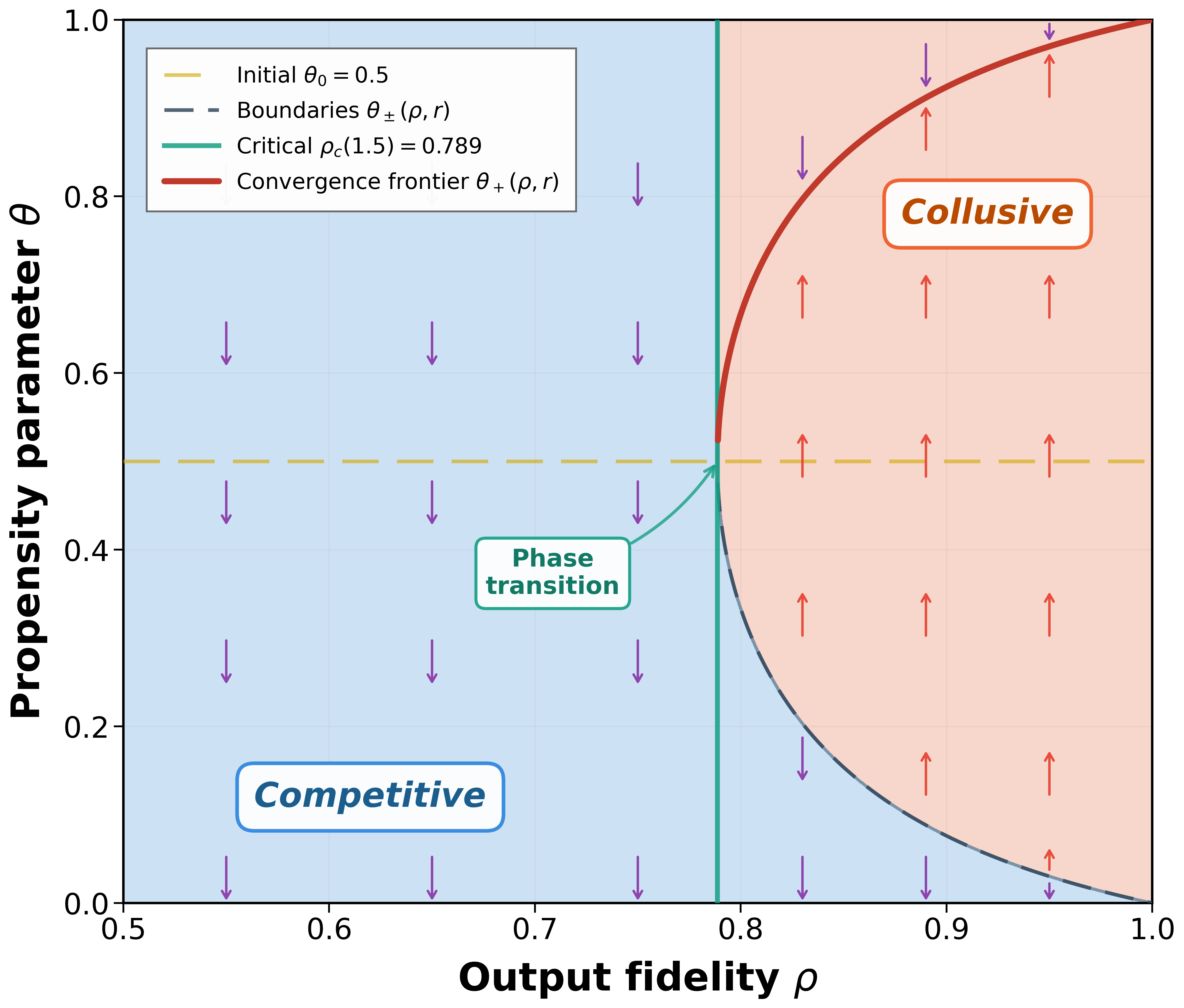
We display the $`(\rho,\theta)`$ parameter space as stated in Proposition [prop:H-dominance] for $`r=1.5`$ and $`\theta_0=1/2`$ in Figure 2. The $`\Delta(\theta) > 0`$ region is bounded by the curves $`\theta_-(\rho,r)`$ and $`\theta_+(\rho,r)`$, which collapse to a single point at $`\theta=1/2`$ when $`\rho=\rho_c(r)`$. For $`\rho<\rho_c(r)`$, no such region exists, the low-price strategy $`L`$ strictly dominates $`H`$ for all propensities $`\theta\in(0,1)`$, always driving the system toward competitive pricing ($`\theta\to 0`$).
The convergence frontier $`\theta_+(\rho,r)`$ illustrates the limit dynamics. Starting from the symmetric initial condition $`\theta_0=1/2`$ (see the horizontal dashed line), the propensity evolves according to the update rule. For any $`\rho\ge\rho_c(r)`$, the system converges to $`\theta_+(\rho,r)`$, which increases monotonically with $`\rho`$ and approaches 1 as $`\rho\to 1`$. This monotonicity implies that higher output fidelity leads to more aggressive collusive pricing in the long run.
The phase transition at $`\rho_c(r)`$ (see the vertical line) highlights the critical role of output fidelity. A small increase in output fidelity from just below to just above $`\rho_c(r)`$ transforms the long-run outcome from purely competitive pricing ($`\theta\to 0`$) to partial collusion ($`\theta\to\theta_+(\rho,r)\ge1/2`$). This discontinuity underscores the sensitivity of collusive outcomes to seemingly minor adjustments in LLM configuration parameters such as sampling temperature or top-$`p`$ filtering.
Finally, we note that perfect output fidelity maximizes the correlation between sellers’ actions and thereby sustains collusion most effectively. As $`\rho`$ decreases toward $`\rho_c(r)`$, the $`\Delta(\theta) > 0`$ region narrows and eventually vanishes, indicating that stochastic noise in LLM outputs disrupts coordination and undermines collusive outcomes. $`\mathchoice{\vcenter{\hrule height .4pt \hbox{\vrule width .4pt height5pt \kern 5pt\vrule width.4pt} \hrule height.4pt}}{\vcenter{\hrule height .4pt \hbox{\vrule width .4pt height5pt \kern 5pt\vrule width.4pt} \hrule height.4pt}}{\vcenter{\hrule height .3pt \hbox{\vrule width .3pt height2.1pt \kern 2.1pt\vrule width.3pt} \hrule height.3pt}}{\vcenter{\hrule height .3pt \hbox{\vrule width .3pt height1.5pt \kern 1.5pt\vrule width.3pt} \hrule height.3pt}}`$
Example [ex:collusion-region] illustrates several key insights from Proposition [prop:convergence-binf]. First, high output fidelity enables collusion. When the LLM’s output fidelity exceeds the critical threshold $`\rho_c(r)`$, a collusive equilibrium emerges and can be selected by the learning dynamics. This finding is particularly concerning for practical applications. In high-stakes tasks such as pricing, decision-makers typically set the LLM decoding temperature to zero (or near zero) to ensure robustness and reproducibility. This contrasts sharply with creative applications, where higher temperatures are preferred to encourage diversity. Low-temperature decoding increases output fidelity $`\rho`$, thereby inadvertently facilitating collusion. Similarly, greater seller adherence to LLM recommendations corresponds to higher effective output fidelity, further amplifying collusion risk. The threshold $`\rho_c(r)`$ provides a quantitative benchmark: maintaining $`\rho < \rho_c(r)`$ through controlled randomness in recommendations would guarantee competitive long-run outcomes, but this runs counter to standard practices that prioritize decision consistency.
Second, collusion emerges even with a moderate initial propensity. In the high-fidelity regime, Proposition [prop:convergence-binf] establishes that if the LLM’s initial propensity $`\theta_0`$ exceeds the threshold $`\theta_-(\rho,r)`$, which lies below $`1/2`$, the learning dynamics converge to the collusive equilibrium $`\theta_+(\rho,r)`$. This condition is likely to be satisfied in practice, where decision-makers typically prompt LLMs with real-world business contexts rather than abstract or hypothetical framings. Two factors contribute to this tendency. First, modern LLMs are pretrained on vast corpora of real-world text, including business literature, case studies, and strategic discussions, which extensively document the profitability of coordinated pricing. This pretraining endows the model with a prior belief that high prices are advantageous when competitors behave similarly. Second, reinforcement learning from human feedback (RLHF) and other alignment procedures tune the model to produce responses that humans find helpful and reasonable, potentially reinforcing such priors if human evaluators or users favor collusive recommendations.
Recent experimental evidence corroborates this prediction. For instance, find that when a strategic game is presented as a “real-world” business scenario, LLM cooperation (i.e., collusion) rates approach 98%, whereas reframing the identical rules as an “imaginary-world” scenario causes these rates to plummet to 37%. Together, these observations suggest that off-the-shelf LLMs deployed for real-world pricing decisions may enter the collusive parameter range at initialization.
Third, the interior nature of the collusive equilibrium has critical implications for detection and regulation. Because $`\theta_+(\rho,r) < 1`$, prices are elevated on average but not perfectly coordinated: occasional low-price recommendations create plausible deniability and complicate detection methods that rely on identifying perfect price correlation. This pattern resembles tacit collusion, where supra-competitive outcomes emerge without explicit agreement or perfectly synchronized behavior, posing challenges for antitrust enforcement that traditionally requires evidence of coordination.
Finite-Batch Regime
In contrast to the large-batch limit, in which estimation noise vanishes, practical LLM retraining operates with finite batches of interaction data. This introduces stochastic fluctuations that persist throughout the learning process and can alter the system’s trajectory. The key distinction from the large-batch regime is that equilibrium selection becomes random. Recall from Proposition [prop:convergence-binf] that in the high-fidelity regime ($`\rho > \rho_c(r)`$), two stable equilibria coexist: competitive pricing ($`\theta = 0`$) and collusive pricing ($`\theta = \theta_+`$). With finite batches, identical initial conditions can lead to either outcome depending on the realized training data. We now analyze this finite-batch regime by returning to the stochastic recursion [eq:logit-recursion].
Specifically, we define the martingale-difference noise
M_{n+1}\;\triangleq\;\overline{D}_n^{(b)}-\Delta(\theta_n).Because the batch-average estimator $`\overline{D}_n^{(b)}`$ is unbiased, we have
\qquad \mathbb{E}[M_{n+1}\mid \theta_n]=0.With the definition of $`M_{n+1}`$, [eq:logit-recursion] becomes
\begin{equation}
\label{eq:SA-form-z}
z_{n+1} = z_n + \gamma_n\bigl(\Delta(\theta_n)+M_{n+1}\bigr),\qquad \theta_n=\sigma(z_n).
\end{equation}For fixed $`\rho\in(1/2,1)`$, Lemma [lem:unbiased-D] implies that $`\overline D_n^{(b)}`$ (and hence $`M_{n+1}`$) has bounded second moments with $`\mathrm{Var}(M_{n+1}\mid\theta_n)=O(1/b)`$.
The recursion [eq:SA-form-z] has a systematic component $`\Delta(\theta_n)`$, which drives the propensity toward its long-run value, and a noise component $`M_{n+1}`$, which introduces random fluctuations around this trend. The systematic component is identical to the large-batch case analyzed in the previous section: the same stable equilibria ($`\theta=0`$ in the low-fidelity regime, and both $`\theta=0`$ and $`\theta_+`$ in the high-fidelity regime) govern the long-run behavior. The batch size $`b`$ affects only the noise variance, leaving this equilibrium structure unchanged. However, when multiple stable equilibria coexist, noise can drive the system across basin boundaries, rendering the ultimate selection among them random. Standard results from stochastic approximation theory can be applied to establish that the propensity $`\theta_n`$ converges almost surely to one of the stable equilibria, though which one depends on the realized noise path. The following proposition formalizes this convergence.
Fix $`r\in(1,2)`$, $`\rho\in(1/2,1)`$, batch size $`b\ge 1`$, a step-size exponent $`\alpha\in(1/2,1]`$, and a scaling constant $`\eta\in(0,1]`$. Let $`\gamma_n=\eta/(n+1)^\alpha`$ and consider the recursion [eq:logit-recursion] from any $`\theta_0\in(0,1)`$. Then $`\theta_n`$ converges almost surely to a (random) equilibrium of [eq:ODE]. Specifically:
-
If $`\rho\in(1/2,\rho_c(r))`$, then $`\theta_n \xrightarrow{\emph{a.s.}} 0`$.
-
If $`\rho=\rho_c(r)`$, then $`\theta_n \xrightarrow{\emph{a.s.}} \theta_\infty`$ where $`\theta_\infty \in \{0,1/2\}`$.
-
If $`\rho\in(\rho_c(r),1)`$, then $`\theta_n \xrightarrow{\emph{a.s.}} \theta_\infty`$ where $`\theta_\infty \in \{0,\theta_+(\rho,r)\}`$.
Proposition [prop:convergence-general] establishes that finite-batch learning converges almost surely. The argument follows the ODE method for stochastic approximation: the recursion tracks the mean-field ODE, and in one dimension, the limit set must reduce to an ODE equilibrium. Standard nonconvergence results further imply that linearly unstable equilibria are selected with probability zero. In the low-fidelity regime ($`\rho<\rho_c(r)`$), the unique long-run outcome is competitive pricing ($`\theta=0`$), so convergence is deterministic despite the stochastic dynamics. At the knife-edge critical regime ($`\rho=\rho_c(r)`$), the ODE admits an additional equilibrium at $`\theta=1/2`$ with one-sided stability, and finite-batch learning can converge to either $`\theta=0`$ or $`\theta=1/2`$ depending on the realized noise path. In the high-fidelity regime ($`\rho>\rho_c(r)`$), both $`\theta=0`$ and $`\theta_+(\rho,r)`$ are locally stable, and which equilibrium is selected depends on the realized sequence of stochastic shocks $`(M_n)_{n\ge 1}`$. This path dependence is the defining feature of the finite-batch regime: identical models with identical initial conditions can converge to different long-run outcomes depending on the random training data encountered during training.
When $`\rho=1`$, the conditional payoff difference is constant: $`\Delta(\theta)=2r-2>0`$ for all $`\theta\in(0,1)`$, so the mean-field ODE [eq:ODE] has $`\theta=1`$ as its unique attracting equilibrium. Proposition [prop:convergence-general] is stated for $`\rho<1`$ because the IPW estimator [eq:D-def] becomes unbounded as $`\theta\to 0`$ or $`\theta\to 1`$ when $`\rho=1`$ (i.e., an “off-policy without exploration” issue). This can be addressed by mild clipping or enforced exploration, replacing $`p_H(\theta)`$ and $`p_L(\theta)`$ in [eq:D-def] with $`\max\{p_H(\theta),\varepsilon\}`$ and $`\max\{p_L(\theta),\varepsilon\}`$ for a small $`\varepsilon>0`$. Under such standard stabilizations, the stochastic recursion continues to track the same ODE and converges to $`\theta=1`$, for $`\rho=1`$ as well.
The preceding analysis shows that convergence occurs but leaves open the question of which equilibrium is selected in the high-fidelity regime. The following proposition characterizes this equilibrium selection and clarifies how the batch size governs the selection probability.
Fix $`r\in(1,2)`$ and $`\rho\in(\rho_c(r),1)`$, and let $`\theta_-(\rho,r)<\theta_+(\rho,r)`$ denote the unstable and stable interior equilibria from Proposition [prop:H-dominance]. Fix step sizes $`\gamma_n=\eta/(n+1)^\alpha`$ with $`\alpha\in(1/2,1]`$ and $`\eta\in(0,1]`$, and consider the stochastic recursion [eq:logit-recursion] with batch size $`b\ge 1`$ from an initial condition $`\theta_0\in(0,1)`$. Define the collusion probability
p_+(b,\theta_0)\;\triangleq\;\mathbb{P}\Bigl(\lim_{n\to\infty}\theta_n=\theta_+(\rho,r)\Bigr).Then the following holds.
-
(Finite-Horizon Tracking with Explicit $`b`$ Dependence). For every $`T>0`$ and every $`\varepsilon>0`$, there exists a constant $`C=C(T,\rho,r,\alpha,\eta)<\infty`$, independent of $`b`$, such that
MATH\mathbb{P}\Bigl(\sup_{0\le t\le T}\bigl|\bar\theta(t)-\theta^{\det}(t)\bigr|>\varepsilon\Bigr)\;\le\;\frac{C}{b\,\varepsilon^2},Click to expand and view morewhere $`\bar\theta(t)\triangleq\sigma(\bar z(t))`$ is the continuous-time interpolation of the stochastic sequence $`(z_n)`$ (as in Lemma [lem:ODE-tracking]) and $`\theta^{\det}(t)`$ is the continuous-time interpolation of the deterministic (large-batch) recursion [eq:deterministic-update-z] started from the same $`\theta_0`$. In particular, $`\sup_{0\le t\le T}|\bar\theta(t)-\theta^{\det}(t)|=O_p(1/\sqrt b)`$.
-
(Lock-In away from the Separatrix). Fix $`\delta\in(0,1/2)`$ and define
MATHK_+(\delta)\triangleq[\theta_-+\delta,\,1-\delta], \qquad K_-(\delta)\triangleq[\delta,\,\theta_- - \delta].Click to expand and view moreThere exist constants $`c_\delta>0`$ and $`C_\delta<\infty`$ such that, for all $`b\ge 1`$,
MATH\sup_{\theta_0\in K_+(\delta)}\bigl(1-p_+(b,\theta_0)\bigr)\;\le\; C_\delta\,e^{-c_\delta\,b\,\delta^2}, \qquad \sup_{\theta_0\in K_-(\delta)}p_+(b,\theta_0)\;\le\; C_\delta\,e^{-c_\delta\,b\,\delta^2}.Click to expand and view moreConsequently, for any fixed $`\theta_0\neq\theta_-`$ we have
MATH\lim_{b\to\infty}p_+(b,\theta_0)=\mathbbm{1}\{\theta_0>\theta_-\}.Click to expand and view more -
(Transition Region Width). For every $`\epsilon\in(0,1/2)`$ and every $`\delta_0\in(0,1/2)`$ with $`\theta_-\in(\delta_0,1-\delta_0)`$, there exists $`K=K(\rho,r,\alpha,\eta,\epsilon,\delta_0)>0`$ such that for all $`b\ge 1`$ and all $`\theta_0\in[\delta_0,1-\delta_0]`$,
MATHp_+(b,\theta_0)\in(\epsilon,1-\epsilon)\quad\Longrightarrow\quad |\theta_0-\theta_-|\;\le\;\frac{K}{\sqrt b}.Click to expand and view more
Proposition [prop:batch-selection] makes precise that equilibrium selection in the finite-batch regime is governed by two forces: deterministic drift and batch-induced noise. Part (i) quantifies finite-horizon tracking of the large-batch recursion, with deviations scaling as $`O_p(1/\sqrt b)`$. Part (ii) turns this tracking into an equilibrium selection statement: starting a fixed margin $`\delta`$ above (below) the unstable threshold $`\theta_-`$, the probability of selecting the “wrong” equilibrium decays at rate $`e^{-c b\delta^2}`$. The proof of Part (ii) is a one-dimensional barrier argument: reaching the wrong basin requires the weighted noise martingale to overcome a deterministic log-odds gap of order $`\delta`$. Part (iii) summarizes the implication for comparative statics: the only initial conditions that yield a nontrivial mixture of competitive and collusive outcomes lie in an $`O(1/\sqrt b)`$ neighborhood of $`\theta_-`$.
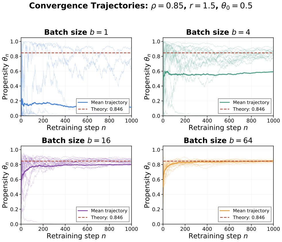
We illustrate the effect of the batch size on equilibrium selection using the same parameter setting as Example [ex:collusion-region]: $`r=1.5`$ and $`\theta_0=1/2`$. We set $`\rho=0.85`$, which exceeds the critical threshold $`\rho_c(1.5)\approx 0.789`$. For these parameters, $`\theta_-\approx 0.154`$ and $`\theta_+\approx 0.846`$. Since the initial propensity $`\theta_0=1/2`$ exceeds $`\theta_-`$, the deterministic dynamics (i.e., the large-batch limit) would converge to the collusive equilibrium $`\theta_+`$. Following standard practice in the stochastic approximation literature, we set the step size as $`\gamma_n=1/(n+1)^\alpha`$. We note that condition (A1) requires $`\alpha\in(1/2,1]`$. We thus set $`\alpha=2/3`$ to ensure practical convergence within the simulation horizon. Figure 3 displays 20 independent trajectories of $`\theta_n`$ for batch sizes $`b\in\{1,4,16,64\}`$, along with their sample means.
Several patterns emerge. First, all trajectories across all batch sizes eventually stabilize, consistent with the almost-sure convergence established in Proposition [prop:convergence-general]. Second, the variance of the trajectories decreases markedly with the batch size. For $`b=1`$, trajectories exhibit substantial volatility and frequently cross the unstable threshold $`\theta_-`$. For $`b=64`$, trajectories remain tightly concentrated around the mean path and converge to the theoretical equilibrium $`\theta_+\approx 0.846`$. Third, the fraction of trajectories converging to the collusive equilibrium $`\theta_+`$ increases with the batch size in this simulation: 15% for $`b=1`$, 70% for $`b=4`$, 95% for $`b=16`$, and 100% for $`b=64`$. This pattern is consistent with Proposition [prop:batch-selection], which predicts that when $`\theta_0>\theta_-`$, the collusion probability rises toward one as batch noise vanishes. $`\mathchoice{\vcenter{\hrule height .4pt \hbox{\vrule width .4pt height5pt \kern 5pt\vrule width.4pt} \hrule height.4pt}}{\vcenter{\hrule height .4pt \hbox{\vrule width .4pt height5pt \kern 5pt\vrule width.4pt} \hrule height.4pt}}{\vcenter{\hrule height .3pt \hbox{\vrule width .3pt height2.1pt \kern 2.1pt\vrule width.3pt} \hrule height.3pt}}{\vcenter{\hrule height .3pt \hbox{\vrule width .3pt height1.5pt \kern 1.5pt\vrule width.3pt} \hrule height.3pt}}`$
 />
/>
Example [ex:batch-size] carries important implications for understanding collusion risk in practice. Proposition [prop:batch-selection] implies that when the initial propensity lies above the unstable threshold $`\theta_-`$, increasing the batch size suppresses noise and pushes the selection probability closer to the large-batch prediction of collusion. In the context of LLM-based pricing, the batch size $`b`$ corresponds to the number of pricing rounds accumulated before each retraining update. In practice, retraining a large language model from scratch is prohibitively expensive, requiring months of computation on thousands of specialized accelerators. Major LLM providers therefore perform full retraining infrequently: OpenAI, Anthropic, and Google typically release major model updates every 6–12 months. Between major releases, models may receive incremental updates via parameter-efficient fine-tuning or retrieval augmentation, but the core model weights, which encode the propensity $`\theta`$ in our model, remain fixed mainly. This operational reality translates directly into large effective batch sizes.
Coupled with the fact that real-world LLMs likely possess initial propensities $`\theta_0>\theta_-`$ owing to pretraining on business corpora and RLHF alignment, Proposition [prop:batch-selection] delivers a striking implication: larger retraining intervals can increase collusion risk by suppressing the noise that might otherwise push the system across the unstable threshold toward competitive pricing.
Conclusion
This paper develops a theoretical framework to analyze the emergence of collusion when sellers delegate pricing decisions to a large language model. Our analysis identifies a fundamental mechanism: the LLM’s shared latent preference creates correlated recommendations across sellers, and a learning process that updates the model’s propensity based on observed performance can drive prices toward collusive levels without any explicit coordination.
Our framework is subject to several limitations that suggest directions for future research. First, the model considers a duopoly setting with two sellers. Extending the analysis to $`N`$ sellers introduces two opposing forces: more sellers increase the probability of at least one recommendation miscoordination, and miscoordinations favor low-price sellers, potentially undermining collusion. Simultaneously, however, the LLM creates market-wide correlation, as all $`N`$ sellers receive signals drawn from the same latent preference, amplifying the monoculture effect. A central research question can be how the critical fidelity threshold $`\rho_c`$ varies with $`N`$: Does market fragmentation protect against, or amplify, LLM-induced collusion?
Second, our model assumes that sellers query the LLM without historical context, so both receive recommendations drawn from the same propensity $`\theta`$. In practice, queries may incorporate historical pricing data, sales outcomes, or competitor behavior. With such context, the LLM could adapt its recommendations to each seller’s history through in-context learning , potentially providing different policies to different sellers within each batch. One seller might receive signals that push toward collusive pricing, while another receives signals that push toward competitive pricing. When these divergent experiences are merged during retraining, the key question is whether policies converge to a common equilibrium or persistently remain heterogeneous. This connects to cutting-edge topics in machine learning, including continual learning, in which models must learn from sequential, potentially conflicting data streams , and catastrophic forgetting, in which training on new data overwrites previously learned knowledge . Understanding how these dynamics interact with the collusion mechanisms identified in this paper presents an important direction for future research.
Online Appendix to
“LLM Collusion”:
Supplementary Derivations and Proofs
Proofs
Proof of Lemma [lem:unbiased-D]. For fixed $`\theta`$, by the law of total expectation,
\begin{align*}
\mathbb{E}[D(\theta)\mid\theta]
&= \frac{1}{p_H(\theta)}\mathbb{E}[\Pi\,\mathbbm{1}\{S=H\}] - \frac{1}{p_L(\theta)}\mathbb{E}[\Pi\,\mathbbm{1}\{S=L\}]\\
&= \frac{\mathbb{P}(S=H)}{p_H(\theta)}\mathbb{E}[\Pi \mid S=H] - \frac{\mathbb{P}(S=L)}{p_L(\theta)}\mathbb{E}[\Pi \mid S=L]\\
&= \mathbb{E}[\Pi \mid S=H] - \mathbb{E}[\Pi \mid S=L] \;=\; \Delta(\theta).
\end{align*}For the boundedness claim, note that payoffs are bounded and, for any fixed $`\rho\in(1/2,1)`$,
\inf_{\theta\in[0,1]}\min\{p_H(\theta),p_L(\theta)\} = 1-\rho \;>\;0,and with $`\Pi_{\max}\triangleq \max\{r, 2r,2+r,2\}=2+r`$, we have $`\bigl|D(\theta)\bigr|\le \Pi_{\max}/(1-\rho)<\infty`$ uniformly in $`\theta`$. $`\mathchoice{\vcenter{\hrule height .4pt \hbox{\vrule width .4pt height5pt \kern 5pt\vrule width.4pt} \hrule height.4pt}}{\vcenter{\hrule height .4pt \hbox{\vrule width .4pt height5pt \kern 5pt\vrule width.4pt} \hrule height.4pt}}{\vcenter{\hrule height .3pt \hbox{\vrule width .3pt height2.1pt \kern 2.1pt\vrule width.3pt} \hrule height.3pt}}{\vcenter{\hrule height .3pt \hbox{\vrule width .3pt height1.5pt \kern 1.5pt\vrule width.3pt} \hrule height.3pt}}`$
Proof of Lemma [lem:ODE-tracking]. We organize the proof into six steps. Steps 1 to 5 establish the tracking statement in part (i) for the log-odds recursion. Step 6 works in propensity space to conclude part (ii).
Step 1: Drift-noise decomposition.
Rewrite the recursion [eq:logit-recursion] as
\begin{equation}
\label{eq:SA-decomposition}
z_{n+1} = z_n + \gamma_n \bigl[\Delta(\theta_n) + M_{n+1}\bigr],
\end{equation}where $`\theta_n = \sigma(z_n)`$ and the noise term is defined as
M_{n+1} := \overline{D}_n^{(b)} - \Delta(\theta_n).By assumption (A2), the sequence $`(M_{n+1})_{n \geq 0}`$ is a martingale difference sequence adapted to the filtration $`(\mathcal{H}_n)_{n \geq 0}`$:
\mathbb{E}[M_{n+1} \mid \mathcal{H}_n] = \mathbb{E}[\overline{D}_n^{(b)} \mid \mathcal{H}_n] - \Delta(\theta_n) = 0.Moreover, by assumption (A3) and the boundedness of $`\Delta(\cdot)`$ established in Lemma [lem:unbiased-D], the second moments are uniformly bounded:
\begin{equation}
\label{eq:noise-bound}
\sup_{n \geq 0} \mathbb{E}[M_{n+1}^2] \le 2\sup_{n}\mathbb{E}[(\overline{D}_n^{(b)})^2] + 2\sup_{\theta \in [0,1]}|\Delta(\theta)|^2 < \infty.
\end{equation}Step 2: Almost-sure convergence of the noise sum.
Define the partial sums $`W_n := \sum_{k=0}^{n-1} \gamma_k M_{k+1}`$. We claim that $`(W_n)_{n \geq 0}`$ converges almost surely to a finite limit.
To see this, observe that $`(W_n,\mathcal{H}_n)_{n \geq 0}`$ is a martingale and
\mathbb{E}[W_n^2] = \sum_{k=0}^{n-1} \gamma_k^2 \, \mathbb{E}[M_{k+1}^2] \le C_M \sum_{k=0}^{n-1} \gamma_k^2,where $`C_M := \sup_k \mathbb{E}[M_{k+1}^2] < \infty`$ by [eq:noise-bound]. Since $`\sum_{k=0}^\infty \gamma_k^2 < \infty`$, the martingale $`(W_n)`$ is $`L^2`$-bounded. By the martingale convergence theorem , $`W_n`$ converges almost surely (and in $`L^2`$) to a finite limit $`W_\infty`$.
Step 3: Regularity of the drift function.
Define $`h: \mathbb{R} \to \mathbb{R}`$ by $`h(z) := \Delta(\sigma(z))`$. We verify that $`h`$ is globally Lipschitz and bounded.
The sigmoid function $`\sigma(z) = (1 + e^{-z})^{-1}`$ is infinitely differentiable with
\sigma'(z) = \sigma(z)\bigl(1 - \sigma(z)\bigr) \in (0, 1/4] \quad \text{for all } z \in \mathbb{R}.By construction, $`\Delta(\theta)`$ admits an explicit rational expression in $`\theta`$, with denominator $`p_H(\theta)p_L(\theta)`$. For $`\rho \in (1/2, 1)`$, Lemma [lem:unbiased-D] shows that $`p_H(\theta), p_L(\theta) \geq 1 - \rho > 0`$ for all $`\theta \in [0,1]`$, so $`\Delta`$ is continuously differentiable on $`[0,1]`$ and $`\sup_{\theta \in [0,1]}|\Delta'(\theta)| < \infty`$. Consequently, $`h = \Delta \circ \sigma`$ is continuously differentiable on $`\mathbb{R}`$ and
|h'(z)| = \bigl|\Delta'(\sigma(z))\bigr|\,\sigma'(z) \le \frac{1}{4}\sup_{\theta \in [0,1]}|\Delta'(\theta)|,which implies a global Lipschitz constant. In addition, $`|h(z)| \le \sup_{\theta \in [0,1]}|\Delta(\theta)|`$ for all $`z`$.
Step 4: Discrete-to-continuous comparison via Gronwall’s inequality.
Fix a horizon $`T > 0`$. For any initial condition $`z \in \mathbb{R}`$, let $`\Phi_t(z)`$ denote the solution to the ODE $`\dot{z} = h(z)`$ at time $`t`$ when starting from $`z(0) = z`$. We compare the discrete sequence $`(z_n)`$ to the ODE trajectory $`(\Phi_{t-t_n}(z_n))_{t \geq t_n}`$.
For $`t \in [t_n, t_{n+1}]`$, the ODE solution starting from $`z_n`$ satisfies
\Phi_{t-t_n}(z_n) = z_n + \int_0^{t-t_n} h\bigl(\Phi_s(z_n)\bigr) \, ds.In particular, setting $`H := \sup_z |h(z)|`$ and $`L`$ to be a global Lipschitz constant for $`h`$, we have
\bigl|\Phi_{\gamma_n}(z_n) - z_n - \gamma_n h(z_n)\bigr|
= \biggl|\int_0^{\gamma_n}\!\!\bigl(h(\Phi_s(z_n)) - h(z_n)\bigr)\,ds\biggr|
\le \int_0^{\gamma_n} L \,|\Phi_s(z_n) - z_n|\,ds
\le \int_0^{\gamma_n} L s H\,ds
= \frac{LH}{2}\,\gamma_n^2.Combining this with [eq:SA-decomposition], the one-step error $`\varepsilon_n := z_{n+1} - \Phi_{\gamma_n}(z_n)`$ satisfies
|\varepsilon_n| \le \gamma_n |M_{n+1}| + \frac{LH}{2}\,\gamma_n^2.Iterating and applying a discrete Gronwall argument yields a uniform bound for the deviation between the interpolated path and the ODE trajectory over $`[t_n,t_n+T]`$ in terms of the martingale increments $`W_m-W_n`$ and the tail sum $`\sum_{k=n}^\infty \gamma_k^2`$.
Step 5: Tracking error decay.
Define the tracking error over a fixed time horizon $`T > 0`$ as
V_n \;:=\; \sup_{0 \leq t \leq T} \bigl|\bar{z}(t_n + t) - \Phi_t(z_n)\bigr|.Let $`N_T(n)`$ denote the number of discrete steps in the time window $`[t_n, t_n + T]`$. Since $`h`$ is globally Lipschitz and bounded, applying the discrete Gronwall inequality to the one-step errors from Step 4 yields a constant $`C_T < \infty`$ (depending only on $`T`$, $`L`$, and $`H`$) such that
V_n \le C_T \biggl( \sup_{m \ge n}\bigl|W_m - W_n\bigr| + \sum_{k=n}^{\infty} \gamma_k^2 \biggr).From Step 2, the partial sums $`W_m := \sum_{k=0}^{m-1} \gamma_k M_{k+1}`$ converge almost surely to a finite limit $`W_\infty`$. Therefore,
\sup_{m \ge n}\bigl|W_m - W_n\bigr| \to 0 \quad \text{a.s.}as $`n \to \infty`$. Since $`\sum_{k=0}^\infty \gamma_k^2 < \infty`$, the tail sum also vanishes: $`\sum_{k=n}^\infty \gamma_k^2 \to 0`$. Combining these estimates yields $`V_n \to 0`$ almost surely, establishing part (i).
Step 6: Limit set characterization.
Let $`z^\star`$ be a limit point of $`(z_n)`$ and let $`z_{n_j} \to z^\star`$ along a subsequence. Then $`\theta_{n_j} := \sigma(z_{n_j}) \to \theta^\star := \sigma(z^\star)`$ with $`\theta^\star \in (0,1)`$. We now work in propensity space.
By a second-order Taylor expansion of $`\sigma`$, there exists $`\xi_n`$ between $`z_n`$ and $`z_{n+1}`$ such that
\theta_{n+1}
= \theta_n + \gamma_n \sigma'(z_n)\,\overline{D}_n^{(b)} + \frac{1}{2}\sigma''(\xi_n)\,\gamma_n^2\bigl(\overline{D}_n^{(b)}\bigr)^2
= \theta_n + \gamma_n \theta_n(1-\theta_n)\,\overline{D}_n^{(b)} + \frac{1}{2}\sigma''(\xi_n)\,\gamma_n^2\bigl(\overline{D}_n^{(b)}\bigr)^2.Write $`\overline{D}_n^{(b)} = \Delta(\theta_n) + M_{n+1}`$ and define
F(\theta) := \theta(1-\theta)\Delta(\theta),\qquad \widetilde M_{n+1} := \theta_n(1-\theta_n)M_{n+1},\qquad r_{n+1} := \frac{1}{2}\sigma''(\xi_n)\,\gamma_n \bigl(\overline{D}_n^{(b)}\bigr)^2.Then the propensity recursion becomes
\theta_{n+1} = \theta_n + \gamma_n\bigl(F(\theta_n) + \widetilde M_{n+1} + r_{n+1}\bigr).Since $`|\sigma''(z)| = |\sigma(z)(1-\sigma(z))(1-2\sigma(z))| \le 1/4`$ for all $`z`$, we have
\sum_{n=0}^\infty \gamma_n |r_{n+1}|
\le \frac{1}{8}\sum_{n=0}^\infty \gamma_n^2 \bigl(\overline{D}_n^{(b)}\bigr)^2
< \infty \quad \text{a.s.},where the almost-sure finiteness follows from (A1) and (A3) by Fubini’s theorem. Moreover, $`(\widetilde M_{n+1})`$ is a martingale difference sequence with uniformly bounded second moments since $`\theta_n(1-\theta_n) \le 1/4`$.
Standard stochastic approximation results imply that the piecewise-linear interpolation of $`(\theta_n)`$ is an asymptotic pseudotrajectory of the ODE $`\dot{\theta} = F(\theta)`$, which is [eq:ODE]. Since $`(\theta_n)`$ is bounded, implies that its $`\omega`$-limit set is internally chain transitive for this one-dimensional flow. In one dimension, any internally chain transitive set must be contained in the equilibrium set $`\{\theta : F(\theta)=0\}`$. Therefore, every limit point $`\theta^\star`$ satisfies $`F(\theta^\star)=0`$. For $`\theta^\star \in (0,1)`$ this reduces to $`\Delta(\theta^\star)=0`$, which is equivalent to $`\Delta(\sigma(z^\star))=0`$. This establishes part (ii) and completes the proof. $`\mathchoice{\vcenter{\hrule height .4pt \hbox{\vrule width .4pt height5pt \kern 5pt\vrule width.4pt} \hrule height.4pt}}{\vcenter{\hrule height .4pt \hbox{\vrule width .4pt height5pt \kern 5pt\vrule width.4pt} \hrule height.4pt}}{\vcenter{\hrule height .3pt \hbox{\vrule width .3pt height2.1pt \kern 2.1pt\vrule width.3pt} \hrule height.3pt}}{\vcenter{\hrule height .3pt \hbox{\vrule width .3pt height1.5pt \kern 1.5pt\vrule width.3pt} \hrule height.3pt}}`$
Proof of Proposition [prop:H-dominance]. Let $`S_i\in\{H,L\}`$ denote the recommendation to Seller $`i`$ and let $`\Pi_i`$ denote Seller $`i`$’s profit in a single period. From Table 1:
\begin{align*}
&(H,H): &&\Pi_1 = 2r,\quad \Pi_2 = 2r,\\
&(H,L): &&\Pi_1 = r,\quad \Pi_2 = 2+r,\\
&(L,H): &&\Pi_1 = 2+r,\quad \Pi_2 = r,\\
&(L,L): &&\Pi_1 = 2,\quad \Pi_2 = 2.
\end{align*}Using the joint probabilities [eq:pHH]–[eq:pLL], the conditional expected profits are
\begin{align}
\mathbb{E}[\Pi_1 \mid S_1 = H, \theta] &= \frac{p_{HH}(\theta) \cdot 2r + p_{HL}(\theta) \cdot r}{p_{HH}(\theta) + p_{HL}(\theta)}, \label{eq:EH-cond-app}\\
\mathbb{E}[\Pi_1 \mid S_1 = L, \theta] &= \frac{p_{LH}(\theta) \cdot (2+r) + p_{LL}(\theta) \cdot 2}{p_{LH}(\theta) + p_{LL}(\theta)}. \label{eq:EL-cond-app}
\end{align}The same expressions hold for Seller 2 by symmetry. Let $`A:=p_{HH}(\theta)`$, $`B:=p_{LL}(\theta)`$, and $`q:=p_{HL}(\theta)=p_{LH}(\theta)=\rho(1-\rho)`$. The condition $`\Delta(\theta)\ge 0`$ is equivalent to
\begin{equation}
\label{eq:ineq-cross-app}
r(2A+q)(q+B) \;\ge\; (A+q)\bigl((r+2)q + 2B\bigr),
\end{equation}which follows by cross-multiplying [eq:EH-cond-app]–[eq:EL-cond-app].
Let $`\kappa\triangleq \rho^2-(1-\rho)^2 = 2\rho-1`$. Then
A=(1-\rho)^2+\kappa\theta,\qquad B=\rho^2-\kappa\theta.Substituting these expressions into [eq:ineq-cross-app] and simplifying yields
\begin{equation}
\label{eq:theta-quadratic-app}
\theta(1-\theta) \;\ge\; K(\rho,r) \;\triangleq\; \frac{(2-r)\,\rho(1-\rho)}{2(r-1)(2\rho-1)^2}.
\end{equation}Define $`s(\rho,r)\triangleq 4K(\rho,r)`$, as in [eq:s-definition]. Then [eq:theta-quadratic-app] is equivalent to $`\theta(1-\theta)\ge s(\rho,r)/4`$.
The function $`f(\theta)=\theta(1-\theta)`$ is concave on $`[0,1]`$ and attains its maximum $`1/4`$ at $`\theta=1/2`$. Consider
g(\theta)\triangleq \theta^2-\theta+\frac{s(\rho,r)}{4}.Then $`\theta(1-\theta)\ge s/4`$ is equivalent to $`g(\theta)\le 0`$. The discriminant of $`g`$ is $`1-s(\rho,r)`$.
Case $`s(\rho,r)>1`$.
Then $`1-s<0`$ and $`g(\theta)>0`$ for all $`\theta`$, so [eq:theta-quadratic-app] never holds and therefore $`\Delta(\theta)<0`$ for all $`\theta\in(0,1)`$.
Case $`s(\rho,r)=1`$.
Then $`g(\theta)=(\theta-1/2)^2`$, so [eq:theta-quadratic-app] holds if and only if $`\theta=1/2`$, implying $`\Delta(1/2)=0`$ and $`\Delta(\theta)<0`$ for $`\theta\ne 1/2`$.
Case $`s(\rho,r)<1`$.
Then $`g`$ has two real roots
\theta_\pm=\frac{1}{2}\pm \frac{1}{2}\sqrt{1-s(\rho,r)},and $`g(\theta)\le 0`$ if and only if $`\theta\in[\theta_-,\theta_+]`$. This implies $`\Delta(\theta)>0`$ for $`\theta\in(\theta_-,\theta_+)`$, with $`\Delta(\theta_\pm)=0`$ and $`\Delta(\theta)<0`$ outside $`[\theta_-,\theta_+]`$. $`\mathchoice{\vcenter{\hrule height .4pt \hbox{\vrule width .4pt height5pt \kern 5pt\vrule width.4pt} \hrule height.4pt}}{\vcenter{\hrule height .4pt \hbox{\vrule width .4pt height5pt \kern 5pt\vrule width.4pt} \hrule height.4pt}}{\vcenter{\hrule height .3pt \hbox{\vrule width .3pt height2.1pt \kern 2.1pt\vrule width.3pt} \hrule height.3pt}}{\vcenter{\hrule height .3pt \hbox{\vrule width .3pt height1.5pt \kern 1.5pt\vrule width.3pt} \hrule height.3pt}}`$
Proof of Proposition [prop:convergence-binf]. The proof proceeds in three parts: (i) establishing almost-sure convergence of the stochastic recursion to the limiting deterministic recursion as $`b \to \infty`$; (ii) deriving the critical fidelity threshold $`\rho_c(r)`$; and (iii) characterizing the long-run behavior of the limiting recursion for all initial conditions $`\theta_0 \in (0,1)`$.
Part I: Convergence to the limiting recursion as $`b \to \infty`$.
Let $`(\theta_n^{(b)})_{n \geq 0}`$ denote the sequence generated by the stochastic recursion [eq:logit-recursion] with batch size $`b`$, and let $`(\theta_n)_{n \geq 0}`$ denote the solution of the limiting recursion [eq:deterministic-update-z] with the same initial condition $`\theta_0`$.
For each $`n \geq 0`$, define the estimation error $`\varepsilon_n^{(b)} := \overline{D}_n^{(b)} - \Delta(\theta_n^{(b)})`$. By Lemma [lem:unbiased-D], conditional on the history $`\mathcal{H}_n`$, the estimator $`\overline{D}_n^{(b)}`$ is an unbiased estimator of $`\Delta(\theta_n^{(b)})`$ with variance $`\mathrm{Var}(\overline{D}_n^{(b)} \mid \mathcal{H}_n) = O(1/b)`$. More precisely, for any fixed $`\rho \in (1/2, 1)`$, there exists a constant $`C_\rho < \infty`$ such that $`\mathrm{Var}(\overline{D}_n^{(b)} \mid \mathcal{H}_n) \leq C_\rho / b`$ uniformly in $`n`$ and $`\theta_n^{(b)} \in (0,1)`$.
We now show that $`\theta_n^{(b)} \to \theta_n`$ almost surely as $`b \to \infty`$, uniformly over any finite horizon. Fix $`N < \infty`$. The stochastic recursion can be written as
z_{n+1}^{(b)} = z_n^{(b)} + \gamma_n \bigl[\Delta(\theta_n^{(b)}) + \varepsilon_n^{(b)}\bigr],while the limiting recursion satisfies
z_{n+1} = z_n + \gamma_n \Delta(\theta_n).Taking differences and using the global Lipschitz continuity of $`h(z) := \Delta(\sigma(z))`$ from Lemma [lem:ODE-tracking], we obtain
|z_{n+1}^{(b)} - z_{n+1}| \leq |z_n^{(b)} - z_n| + \gamma_n L |z_n^{(b)} - z_n| + \gamma_n |\varepsilon_n^{(b)}|,where $`L`$ is a global Lipschitz constant of $`h`$.
Iterating this bound and applying the discrete Gronwall inequality yields
\max_{0 \leq n \leq N} |z_n^{(b)} - z_n| \leq \exp\Bigl(L \sum_{k=0}^{N-1} \gamma_k\Bigr) \sum_{k=0}^{N-1} \gamma_k |\varepsilon_k^{(b)}|.To upgrade to almost sure convergence in $`b`$, we work under a natural coupling where, at each step $`k`$, the batch of size $`b`$ is the prefix of an infinite i.i.d. stream of interaction rounds. We then use the uniform boundedness of the per-round estimator. For fixed $`\rho\in(1/2,1)`$, Lemma [lem:unbiased-D] implies that $`D(\theta)`$ is uniformly bounded over $`\theta\in[0,1]`$, so there exists $`B_\rho<\infty`$ such that $`|D(\theta)|\le B_\rho`$ almost surely for all $`\theta\in[0,1]`$. Consequently, conditional on $`\mathcal H_k`$, the estimation error $`\varepsilon_k^{(b)}`$ is an average of $`b`$ independent, mean-zero, bounded random variables, and Hoeffding’s inequality yields a constant $`c_\rho>0`$ such that for any $`\delta>0`$,
\mathbb{P}\Bigl(|\varepsilon_k^{(b)}|>\delta \,\big|\, \mathcal H_k\Bigr)\le 2\exp\bigl(-c_\rho b\delta^2\bigr).Taking expectations and applying a union bound over $`k=0,1,\ldots,N-1`$ gives
\mathbb{P}\Bigl(\max_{0\le k\le N-1}|\varepsilon_k^{(b)}|>b^{-1/3}\Bigr)
\le 2N\exp\bigl(-c_\rho b^{1/3}\bigr).Since $`\sum_{b=1}^\infty 2N\exp(-c_\rho b^{1/3})<\infty`$, the Borel–Cantelli lemma implies that $`\max_{0\le k\le N-1}|\varepsilon_k^{(b)}|\le b^{-1/3}`$ eventually almost surely as $`b\to\infty`$. On this event,
\max_{0 \leq n \leq N} |z_n^{(b)} - z_n|
\le \exp\Bigl(L \sum_{k=0}^{N-1} \gamma_k\Bigr)\,b^{-1/3}\sum_{k=0}^{N-1}\gamma_k
\xrightarrow{b\to\infty} 0almost surely. Since $`\sigma`$ is Lipschitz with constant $`1/4`$, this implies $`\max_{0 \leq n \leq N} |\theta_n^{(b)} - \theta_n|\to 0`$ almost surely. Since $`N`$ was arbitrary, a diagonalization argument yields almost-sure convergence uniformly on finite horizons.
Part II: Derivation of the critical fidelity threshold.
By Proposition [prop:H-dominance], the sign of $`\Delta(\theta)`$ on the interior $`(0,1)`$ is determined by the statistic $`s(\rho, r)`$ defined in [eq:s-definition]. The critical case, where $`\Delta(\theta) = 0`$ has a unique interior solution at $`\theta = 1/2`$, occurs when $`s(\rho, r) = 1`$, i.e.,
\frac{2(2-r)\rho(1-\rho)}{(r-1)(2\rho-1)^2} = 1.Cross-multiplying and rearranging yields the quadratic equation
2(2-r)\rho(1-\rho) = (r-1)(2\rho - 1)^2.Expanding both sides:
\begin{align*}
\text{LHS} &= 2(2-r)\rho - 2(2-r)\rho^2 = (4 - 2r)\rho - (4 - 2r)\rho^2, \\
\text{RHS} &= (r-1)(4\rho^2 - 4\rho + 1) = (4r - 4)\rho^2 - (4r - 4)\rho + (r - 1).
\end{align*}Collecting terms:
0 = \bigl[(4r - 4) + (4 - 2r)\bigr]\rho^2 - \bigl[(4r - 4) + (4 - 2r)\bigr]\rho + (r - 1).Simplifying the coefficient: $`(4r - 4) + (4 - 2r) = 2r`$, so
2r\rho^2 - 2r\rho + (r - 1) = 0.Dividing by $`2r`$ and applying the quadratic formula:
\rho = \frac{1 \pm \sqrt{1 - 2(r-1)/r}}{2} = \frac{1 \pm \sqrt{(2-r)/r}}{2}.Since $`\rho \in (1/2, 1]`$ and $`r \in (1, 2)`$ implies $`(2-r)/r \in (0, 1)`$, we have $`\sqrt{(2-r)/r} \in (0, 1)`$. The solution $`\rho_- = (1 - \sqrt{(2-r)/r})/2 < 1/2`$ lies outside the feasible range, so the unique critical threshold is
\rho_c(r) = \frac{1 + \sqrt{(2-r)/r}}{2}.Part III: Long-run behavior of the limiting recursion.
We now characterize the convergence of $`(\theta_n)_{n \geq 0}`$ as $`n \to \infty`$ for each regime of $`\rho`$.
Write $`h(z)\triangleq \Delta(\sigma(z))`$, so the limiting recursion is $`z_{n+1}=z_n+\gamma_n h(z_n)`$ with $`\theta_n=\sigma(z_n)`$. Under our step-size choice, $`0<\gamma_n\le \eta\le 1`$.
We first record a monotonicity property that prevents spurious basin crossings in the deterministic recursion. For $`\rho\in(1/2,1)`$, one can simplify the payoff difference to
\Delta(\theta)=2(r-1)-\frac{r\rho(1-\rho)}{p_H(\theta)p_L(\theta)},
\qquad
p_H(\theta)=(1-\rho)+(2\rho-1)\theta,
\qquad
p_L(\theta)=1-p_H(\theta).Differentiating and using $`\sigma'(z)=\sigma(z)(1-\sigma(z))`$ yields, for $`\rho\in(1/2,1)`$,
|h'(z)|
=\bigl|\Delta'(\sigma(z))\bigr|\,\sigma'(z)
= r\,\frac{t(z)\,|2\sigma(z)-1|}{(1+t(z))^2}
\le \frac{r}{4}
\quad\text{for all }z\in\mathbb R,where $`t(z)\triangleq \frac{(2\rho-1)^2\sigma(z)(1-\sigma(z))}{\rho(1-\rho)}`$ and we used $`x/(1+x)^2\le 1/4`$ for all $`x\ge 0`$. When $`\rho=1`$, we have $`h(z)\equiv 2r-2`$, so $`|h'(z)|=0`$ and the same bound holds. Therefore $`h`$ is globally Lipschitz with constant $`L:=r/4<1/2`$. For each $`n`$, define the update map $`T_n(z):=z+\gamma_n h(z)`$. For any $`z\le z'`$,
T_n(z')-T_n(z)
=(z'-z)+\gamma_n\bigl(h(z')-h(z)\bigr)
\ge (1-\gamma_n L)(z'-z)
\ge 0,so $`T_n`$ is increasing. In particular, if $`h(\bar z)=0`$ and $`z_n\ge \bar z`$, then $`z_{n+1}=T_n(z_n)\ge T_n(\bar z)=\bar z`$.
Case 1: Low-fidelity regime ($`\rho < \rho_c(r)`$).
By Proposition [prop:H-dominance], $`s(\rho, r) > 1`$ implies $`\Delta(\theta) < 0`$ for all $`\theta \in (0, 1)`$. The limiting recursion satisfies
z_{n+1} = z_n + \gamma_n \Delta(\theta_n) < z_n,so $`(z_n)_{n \geq 0}`$ is strictly decreasing. Since $`\Delta(\theta)`$ is bounded away from zero on any compact subset of $`(0, 1)`$ and $`\sum_n \gamma_n = \infty`$, we have $`z_n \to -\infty`$ and hence $`\theta_n = \sigma(z_n) \to 0`$.
Case 2: Critical regime ($`\rho = \rho_c(r)`$).
Here $`s(\rho, r) = 1`$, so $`\Delta(1/2) = 0`$ and $`\Delta(\theta) < 0`$ for all $`\theta \in (0, 1) \setminus \{1/2\}`$.
If $`\theta_0 = 1/2`$, then $`\Delta(\theta_0) = 0`$ implies $`z_1 = z_0 + \gamma_0 \cdot 0 = z_0`$, and by induction $`z_n = z_0`$ for all $`n`$, so $`\theta_n \equiv 1/2`$.
If $`\theta_0 < 1/2`$ (equivalently, $`z_0 < 0`$), then $`\Delta(\theta_0) < 0`$, so $`z_1 < z_0 < 0`$. Since $`\Delta(\theta) < 0`$ for all $`\theta \neq 1/2`$, the sequence $`(z_n)`$ remains negative and strictly decreasing. By the same argument as Case 1, $`z_n \to -\infty`$ and $`\theta_n \to 0`$.
If $`\theta_0 > 1/2`$ (equivalently, $`z_0 > 0`$), then
$`\Delta(\theta_0) < 0`$, so $`z_1
Case 3: High-fidelity regime ($`\rho_c(r) < \rho < 1`$).
By Proposition [prop:H-dominance], $`s(\rho, r) < 1`$ implies the existence of thresholds $`\theta_-(\rho, r) < 1/2 < \theta_+(\rho, r)`$ such that
\Delta(\theta) \begin{cases}
< 0, & \theta \in (0, \theta_-), \\
= 0, & \theta \in \{\theta_-, \theta_+\}, \\
> 0, & \theta \in (\theta_-, \theta_+), \\
< 0, & \theta \in (\theta_+, 1).
\end{cases}Subcase 3(a): $`\theta_0 \in (0, \theta_-)`$. Then
$`z_0 Subcase 3(b): $`\theta_0 \in (\theta_-, 1)`$. Then $`z_0>z_-`$, and
since $`h(z_-)=0`$ and $`T_n`$ is increasing, we have $`z_n>z_-`$ for
all $`n`$. Let $`z_+:=\log\!\bigl(\theta_+/(1-\theta_+)\bigr)`$. The
sign pattern of $`\Delta`$ implies $`h(z)>0`$ for $`z\in(z_-,z_+)`$ and
$`h(z)<0`$ for $`z>z_+`$. Therefore, if $`z_n\le z_+`$ then
$`z_{n+1}\ge z_n`$, and if $`z_n\ge z_+`$ then $`z_{n+1}\le z_n`$. In
either case, the recursion moves toward $`z_+`$. If $`z_n`$ crosses $`z_+`$ only finitely many times, then eventually it
stays on one side of $`z_+`$ and is monotone, hence it converges to some
limit $`z^\star`$. If $`h(z^\star)\neq 0`$, then by continuity there
exists $`c>0`$ such that $`|h(z_n)|\ge c`$ for all $`n`$ large enough,
which implies $`|z_{n+1}-z_n|=\gamma_n|h(z_n)|\ge c\gamma_n`$
eventually. Since $`\sum_n\gamma_n=\infty`$, this contradicts
convergence of $`(z_n)`$. Therefore $`h(z^\star)=0`$, and given
$`z_n>z_-`$ for all $`n`$ this forces $`z^\star=z_+`$. If $`z_n`$ crosses $`z_+`$ infinitely many times, let
$`H:=\sup_{z\in\mathbb R}|h(z)|<\infty`$. At each crossing between $`n`$
and $`n+1`$, the point $`z_+`$ lies between $`z_n`$ and $`z_{n+1}`$, so Since $`\gamma_n\to 0`$, the distance to $`z_+`$ at crossing times tends
to $`0`$. Between crossings, the recursion is monotone and stays between
$`z_+`$ and the most recent crossing value, so the distance to $`z_+`$
is bounded by the corresponding crossing distance. Therefore
$`|z_n-z_+|\to 0`$ and $`z_n\to z_+`$. In both cases, $`z_n\to z_+`$ and therefore
$`\theta_n=\sigma(z_n)\to \theta_+(\rho,r)`$. Case 4: Perfect-fidelity regime ($`\rho = 1`$). When $`\rho = 1`$, only the outcomes $`(H, H)`$ and $`(L, L)`$ occur
(since recommendations match the latent mode with probability one). The
conditional payoff difference becomes for all $`\theta \in (0, 1)`$, since $`r > 1`$. Thus $`z_{n+1} = z_n + \gamma_n(2r - 2) > z_n`$ for all $`n`$, and since
$`\sum_n \gamma_n = \infty`$, we have $`z_n \to +\infty`$ and
$`\theta_n \to 1`$. This completes the proof of
Proposition [prop:convergence-binf].
$`\mathchoice{\vcenter{\hrule height .4pt
\hbox{\vrule width .4pt height5pt \kern 5pt\vrule width.4pt} \hrule height.4pt}}{\vcenter{\hrule height .4pt
\hbox{\vrule width .4pt height5pt \kern 5pt\vrule width.4pt} \hrule height.4pt}}{\vcenter{\hrule height .3pt
\hbox{\vrule width .3pt height2.1pt \kern 2.1pt\vrule width.3pt} \hrule height.3pt}}{\vcenter{\hrule height .3pt
\hbox{\vrule width .3pt height1.5pt \kern 1.5pt\vrule width.3pt} \hrule height.3pt}}`$ Proof of Proposition
[prop:convergence-general].
Recall the stochastic approximation form
[eq:SA-form-z]: The step sizes $`\gamma_n=\eta/(n+1)^\alpha`$ satisfy
$`\sum_n\gamma_n=\infty`$ and $`\sum_n\gamma_n^2<\infty`$ because
$`\alpha\in(1/2,1]`$. For fixed $`\rho\in(1/2,1)`$,
Lemma [lem:unbiased-D] implies
$`\mathbb{E}[M_{n+1}\mid \mathcal H_n]=0`$ and
$`\sup_n \mathbb{E}[M_{n+1}^2]<\infty`$. Define the martingale partial sums
$`W_n \triangleq \sum_{k=0}^{n-1}\gamma_k M_{k+1}`$. Since
$`\sum_k\gamma_k^2<\infty`$ and the conditional second moments of
$`M_{k+1}`$ are uniformly bounded, $`(W_n)`$ is $`L^2`$ bounded and
hence converges almost surely to a finite limit $`W_\infty`$ .
Consequently, Because $`\rho<1`$,
Proposition [prop:H-dominance] implies
$`\Delta(1)<0`$. By continuity of $`\Delta`$ on $`[0,1]`$, there exist
$`\bar\theta\in(0,1)`$ and $`c_1>0`$ such that
$`\Delta(\theta)\le -c_1`$ for all $`\theta\in[\bar\theta,1]`$. If
$`\theta_n\to 1`$, then $`\theta_n\ge \bar\theta`$ for all large $`n`$,
and [eq:z-decomposition-convergence-general]
would imply which contradicts $`\theta_n=\sigma(z_n)\to 1`$. Therefore,
$`\mathbb{P}(\theta_n\to 1)=0`$. Using the first-order expansion
[eq:theta-firstorder] and the
definition of $`M_{n+1}`$, we can write where the remainder satisfies $`|r_{n+1}|\le C\gamma_n^2`$ for a
constant $`C`$ that depends only on $`(\rho,r)`$ and the payoff bounds.
Since $`\sum_n\gamma_n^2<\infty`$, we also have
$`\sum_n |r_{n+1}|<\infty`$. The drift
$`g(\theta)\triangleq \theta(1-\theta)\Delta(\theta)`$ is continuously
differentiable on $`[0,1]`$ for $`\rho\in(1/2,1)`$, hence Lipschitz.
Since $`\theta_n\in(0,1)`$ is bounded, standard ODE-method results for
stochastic approximation applied to
[eq:theta-SA-convergence-general]
imply that $`\theta_n`$ converges almost surely to an equilibrium of the
ODE [eq:ODE] . The equilibria of [eq:ODE] are $`\theta\in\{0,1\}`$ and any
interior $`\theta^\star`$ satisfying $`\Delta(\theta^\star)=0`$.
Proposition [prop:H-dominance] characterizes
the interior zeros. If $`\rho\in(1/2,\rho_c(r))`$, then $`\Delta(\theta)<0`$ for all
$`\theta\in(0,1)`$, so the only equilibria are $`\theta\in\{0,1\}`$.
Since $`\mathbb{P}(\theta_n\to 1)=0`$ by Step 2, we obtain
$`\theta_n\to 0`$ almost surely. If $`\rho=\rho_c(r)`$, then $`\Delta(\theta)=0`$ if and only if
$`\theta=1/2`$, so the equilibria are $`\theta\in\{0,1/2,1\}`$.
Step 2 rules out $`\theta_n\to 1`$, hence
$`\theta_\infty\in\{0,1/2\}`$ almost surely. If $`\rho\in(\rho_c(r),1)`$, then $`\Delta(\theta)=0`$ if and only
if $`\theta\in\{\theta_-(\rho,r),\theta_+(\rho,r)\}`$, so the
equilibria are $`\theta\in\{0,\theta_-,\theta_+,1\}`$. Step 2 rules
out $`\theta_n\to 1`$. Moreover, $`\theta_-(\rho,r)`$ is linearly
unstable for [eq:ODE], and the noise in
[eq:theta-SA-convergence-general]
is nondegenerate on any neighborhood of $`\theta_-`$ for fixed
$`b`$. Standard nonconvergence results for stochastic approximation
then imply $`\mathbb{P}(\theta_n\to \theta_-)=0`$, so
$`\theta_\infty\in\{0,\theta_+(\rho,r)\}`$ almost surely. $`\mathchoice{\vcenter{\hrule height .4pt
\hbox{\vrule width .4pt height5pt \kern 5pt\vrule width.4pt} \hrule height.4pt}}{\vcenter{\hrule height .4pt
\hbox{\vrule width .4pt height5pt \kern 5pt\vrule width.4pt} \hrule height.4pt}}{\vcenter{\hrule height .3pt
\hbox{\vrule width .3pt height2.1pt \kern 2.1pt\vrule width.3pt} \hrule height.3pt}}{\vcenter{\hrule height .3pt
\hbox{\vrule width .3pt height1.5pt \kern 1.5pt\vrule width.3pt} \hrule height.3pt}}`$ Proof of Proposition
[prop:batch-selection].
Throughout, write $`h(z)\triangleq \Delta(\sigma(z))`$ so that the
stochastic recursion in log-odds form is where $`M_{n+1}\triangleq \overline D_n^{(b)}-\Delta(\theta_n)`$ is a
martingale-difference term with
$`\mathbb{E}[M_{n+1}\mid \mathcal H_n]=0`$. Fix $`T>0`$ and let
$`N(T)\triangleq \min\{n:\sum_{k=0}^{n-1}\gamma_k\ge T\}`$. Let
$`z_n^{\det}`$ denote the deterministic recursion
[eq:deterministic-update-z]
and write $`\theta_n^{\det}\triangleq \sigma(z_n^{\det})`$. Define the
error $`e_n\triangleq z_n-z_n^{\det}`$, which satisfies Define the martingale partial sums
$`W_m\triangleq \sum_{k=0}^{m-1}\gamma_k M_{k+1}`$, with $`W_0=0`$, and
set $`u_n\triangleq e_n-W_n`$. Then As shown in the proof of
Proposition [prop:convergence-binf],
$`h`$ is globally Lipschitz on $`\mathbb{R}`$ with some constant
$`L<\infty`$. Let $`W_\star\triangleq \max_{0\le m\le N(T)}|W_m|`$. For
$`n\le N(T)`$, Iterating this inequality and using
$`\sum_{k=0}^{N(T)-1}\gamma_k\le T+\gamma_0\le T+1`$ yields Since $`e_n=u_n+W_n`$, we obtain Because $`\overline D_n^{(b)}`$ is a batch average of bounded per-round
statistics (Lemma [lem:unbiased-D]), there exists
$`V<\infty`$ depending only on $`(\rho,r)`$ such that Therefore, By Doob’s $`L^2`$ maximal inequality, Using that $`\sigma`$ is $`1/4`$ Lipschitz, we have
$`|\theta_n-\theta_n^{\det}|\le \frac{1}{4}|e_n|`$, hence Passing from discrete time to the interpolations $`\bar\theta(t)`$ and
$`\theta^{\det}(t)`$ on $`t\in[0,T]`$ changes only constants, because
the interpolation error is $`O(\max_{n\le N(T)}\gamma_n)`$ and does not
depend on $`b`$. This yields the displayed bound in Part (i) and the
$`O_p(1/\sqrt b)`$ statement follows. Fix $`\delta\in(0,1/2)`$ and recall Write By
Proposition [prop:convergence-general],
in this regime $`\theta_n`$ converges almost surely, and the only
possible limits are $`0`$ and $`\theta_+(\rho,r)`$. Step 1: A maximal inequality for the weighted martingale noise. Write
the batch estimator as an average of $`b`$ i.i.d. per-round scores.
Define so that
$`\overline D_n^{(b)}=\frac{1}{b}\sum_{\ell=1}^b \widetilde D_n^{(\ell)}`$.
Conditional on $`\mathcal H_n`$, the random variables
$`(\widetilde D_n^{(\ell)})_{\ell=1}^b`$ are i.i.d. with mean
$`\Delta(\theta_n)`$. By
Lemma [lem:unbiased-D], there exist
constants $`\underline D<\overline D`$ depending only on $`(\rho,r)`$
such that $`\underline D\le \widetilde D_n^{(\ell)}\le \overline D`$
almost surely for all $`n`$ and $`\ell`$. Consequently, Hoeffding’s
lemma implies that for all $`\lambda\in\mathbb R`$, Define the weighted martingale Fix $`\lambda>0`$ and define Using [eq:batch-selection-subg]
and iterated expectations, $`(\mathcal E_n(\lambda),\mathcal H_n)`$ is a
nonnegative supermartingale with $`\mathbb E[\mathcal E_0(\lambda)]=1`$.
By Ville’s inequality, Optimizing over $`\lambda`$ yields Therefore, for every $`t>0`$, Step 2: A deterministic barrier lemma. Define the down-crossing and
up-crossing times of the unstable log-odds threshold $`z_-`$, Claim (Barrier bound for separatrix crossings). Fix
$`\delta\in(0,1/2)`$ such that $`\theta_- - \delta`$ and
$`\theta_-+\delta`$ lie in $`(0,1)`$, and define If $`z_0\ge z_\delta^+`$ and $`\tau_-<\infty`$, then
$`\sup_{n\ge 0}|W_n|\ge (\underline z_\delta-z_-)/2`$. If $`z_0\le z_\delta^-`$ and $`\tau_+<\infty`$, then
$`\sup_{n\ge 0}|W_n|\ge (z_- - z_\delta^-)/2`$. Proof. Part (a). Assume $`z_0\ge z_\delta^+`$ and $`\tau_-<\infty`$.
Define the last time before $`\tau_-`$ at which the process is at or
above $`\underline z_\delta`$, Then $`z_{\tau_\delta}\ge \underline z_\delta`$ and
$`z_{\tau_\delta+1}<\underline z_\delta`$. If $`z_{\tau_\delta}\le z_+`$, then for every $`k`$ with
$`\tau_\delta\le k<\tau_-`$ we have $`z_- On $`\{\tau_-<\infty\}`$, the middle term is nonnegative, so If $`\sup_n|W_n|<(\underline z_\delta-z_-)/2`$, then
$`W_{\tau_\delta}\le \sup_n|W_n|<(\underline z_\delta-z_-)/2`$ and hence which contradicts $`\sup_n|W_n|<(\underline z_\delta-z_-)/2`$. If instead $`z_{\tau_\delta}> z_+`$, define $`T_n(z):=z+\gamma_n h(z)`$.
As shown in the proof of
Proposition [prop:convergence-binf],
$`|h'(z)|\le r/4`$ for all $`z`$ and since $`\gamma_n\le 1`$ this
implies $`T_n`$ is increasing. Because $`T_{\tau_\delta}(z_+)=z_+`$ and
$`z_{\tau_\delta}\ge z_+`$, we obtain
$`T_{\tau_\delta}(z_{\tau_\delta})\ge z_+`$. Therefore, Since $`\underline z_\delta\le z_{\mathrm{mid}}=(z_-+z_+)/2`$, we have
$`z_+-\underline z_\delta\ge \underline z_\delta-z_-`$. Using
$`|W_{\tau_\delta+1}-W_{\tau_\delta}|\le |W_{\tau_\delta+1}|+|W_{\tau_\delta}|\le 2\sup_n|W_n|`$
yields $`\sup_n|W_n|\ge (\underline z_\delta-z_-)/2`$. Part (b). Assume $`z_0\le z_\delta^-`$ and $`\tau_+<\infty`$. Define
the last time before $`\tau_+`$ at which the process is at or below
$`z_\delta^-`$, Then $`z_{\widehat\tau_\delta}\le z_\delta^-`$, and for every $`k`$ with
$`\widehat\tau_\delta\le k<\tau_+`$ we have $`z_\delta^- and the middle term is nonpositive, so If $`\sup_n|W_n|<(z_- - z_\delta^-)/2`$, then
$`W_{\widehat\tau_\delta}\ge -\sup_n|W_n|>-(z_- - z_\delta^-)/2`$ and
thus contradicting $`\sup_n|W_n|<(z_- - z_\delta^-)/2`$.
$`\mathchoice{\vcenter{\hrule height .4pt
\hbox{\vrule width .4pt height5pt \kern 5pt\vrule width.4pt} \hrule height.4pt}}{\vcenter{\hrule height .4pt
\hbox{\vrule width .4pt height5pt \kern 5pt\vrule width.4pt} \hrule height.4pt}}{\vcenter{\hrule height .3pt
\hbox{\vrule width .3pt height2.1pt \kern 2.1pt\vrule width.3pt} \hrule height.3pt}}{\vcenter{\hrule height .3pt
\hbox{\vrule width .3pt height1.5pt \kern 1.5pt\vrule width.3pt} \hrule height.3pt}}`$ Step 3: Conclude the exponential bounds. Fix $`\delta\in(0,1/2)`$. If $`\theta_0\in K_+(\delta)`$ then $`z_0\ge z_\delta^+`$. On the event
$`\{\theta_n\to 0\}`$ we have $`z_n\to-\infty`$, hence
$`\tau_-<\infty`$. Therefore, using Step 2(a) and
[eq:batch-selection-W-max], Similarly, if $`\theta_0\in K_-(\delta)`$ then $`z_0\le z_\delta^-`$. On
the event $`\{\theta_n\to\theta_+\}`$ we have $`z_n\to z_+>z_-`$, hence
$`\tau_+<\infty`$. Step 2(b) and
[eq:batch-selection-W-max]
give Finally, note that and $`\underline z_\delta-z_-=(z_\delta^+-z_-)\wedge((z_+-z_-)/2)`$.
This implies the displayed bounds in Part (ii) after absorbing constants
into $`c_\delta`$ and $`C_\delta`$. For any fixed
$`\theta_0\ne\theta_-`$, choose $`\delta>0`$ such that
$`\theta_0\in K_+(\delta)`$ when $`\theta_0>\theta_-`$ and
$`\theta_0\in K_-(\delta)`$ when $`\theta_0<\theta_-`$. Letting
$`b\to\infty`$ then yields
$`\lim_{b\to\infty}p_+(b,\theta_0)=\mathbbm{1}\{\theta_0>\theta_-\}`$. Fix $`\epsilon\in(0,1/2)`$ and $`\delta_0\in(0,1/2)`$ with
$`\theta_-\in(\delta_0,1-\delta_0)`$. Set Let $`\theta_0\in[\delta_0,1-\delta_0]`$ and define
$`\delta:=\min\{\tfrac12|\theta_0-\theta_-|,\delta_0\}`$. If
$`\theta_0=\theta_-`$, the conclusion is immediate, so assume
$`\theta_0\ne\theta_-`$. If $`\theta_0>\theta_-`$ then
$`\theta_0\in K_+(\delta)`$, and if $`\theta_0<\theta_-`$ then
$`\theta_0\in K_-(\delta)`$. For $`\delta\le \delta_0`$ we have Therefore, by the bounds established in Part (ii), for all $`b\ge 1`$, Rearranging yields Define Then $`\delta\le A/\sqrt b`$. If $`|\theta_0-\theta_-|\le 2\delta_0`$,
we have $`\delta=\tfrac12|\theta_0-\theta_-|`$, so
$`|\theta_0-\theta_-|=2\delta\le 2A/\sqrt b`$. If instead
$`|\theta_0-\theta_-|>2\delta_0`$, we have $`\delta=\delta_0`$, so
$`\delta_0\le A/\sqrt b`$ and hence $`b\le A^2/\delta_0^2`$. Since
$`|\theta_0-\theta_-|\le 1`$, this implies
$`|\theta_0-\theta_-|\le (A/\delta_0)/\sqrt b`$. Taking
$`K:=A/\delta_0`$ completes the proof.
$`\mathchoice{\vcenter{\hrule height .4pt
\hbox{\vrule width .4pt height5pt \kern 5pt\vrule width.4pt} \hrule height.4pt}}{\vcenter{\hrule height .4pt
\hbox{\vrule width .4pt height5pt \kern 5pt\vrule width.4pt} \hrule height.4pt}}{\vcenter{\hrule height .3pt
\hbox{\vrule width .3pt height2.1pt \kern 2.1pt\vrule width.3pt} \hrule height.3pt}}{\vcenter{\hrule height .3pt
\hbox{\vrule width .3pt height1.5pt \kern 1.5pt\vrule width.3pt} \hrule height.3pt}}`$\max\{|z_n-z_+|,\ |z_{n+1}-z_+|\}\le |z_{n+1}-z_n|=\gamma_n|h(z_n)|\le \gamma_n H.\Delta(\theta) = \mathbb{E}[\Pi \mid S = H] - \mathbb{E}[\Pi \mid S = L] = 2r - 2 > 0z_{n+1} = z_n + \gamma_n\bigl(\Delta(\theta_n)+M_{n+1}\bigr),
\qquad \theta_n=\sigma(z_n).Step 1: Noise summability.
\begin{equation}
\label{eq:z-decomposition-convergence-general}
z_n = z_0 + \sum_{k=0}^{n-1}\gamma_k\,\Delta(\theta_k) + W_n.
\end{equation}Step 2: Excluding $`\theta_n\to 1`$.
z_n \le z_0 - c_1\sum_{k=0}^{n-1}\gamma_k + W_n \to -\infty,Step 3: Convergence to ODE equilibria.
\begin{equation}
\label{eq:theta-SA-convergence-general}
\theta_{n+1} = \theta_n + \gamma_n\Bigl(\theta_n(1-\theta_n)\Delta(\theta_n) + \theta_n(1-\theta_n)M_{n+1}\Bigr) + r_{n+1},
\end{equation}Step 4: Identifying the possible limits.
z_{n+1}=z_n+\gamma_n\bigl(h(z_n)+M_{n+1}\bigr),\qquad \theta_n=\sigma(z_n),Part (i).
e_{n+1}
=e_n+\gamma_n\bigl(h(z_n)-h(z_n^{\det})\bigr)+\gamma_n M_{n+1}.u_{n+1}=u_n+\gamma_n\bigl(h(z_n)-h(z_n^{\det})\bigr).|u_{n+1}|
\le |u_n|+\gamma_n L |e_n|
=|u_n|+\gamma_n L |u_n+W_n|
\le (1+L\gamma_n)|u_n|+L\gamma_n W_\star.\max_{0\le n\le N(T)}|u_n|\le e^{L(T+1)}\,L(T+1)\,W_\star.\max_{0\le n\le N(T)}|e_n|
\le \bigl(1+e^{L(T+1)}L(T+1)\bigr)\,W_\star.\mathbb{E}\bigl[M_{n+1}^2\mid \mathcal H_n\bigr]\le \frac{V}{b}\qquad\text{a.s. for all }n.\mathbb{E}[W_{N(T)}^2]
=\sum_{k=0}^{N(T)-1}\gamma_k^2\,\mathbb{E}[M_{k+1}^2]
\le \frac{V}{b}\sum_{k=0}^{N(T)-1}\gamma_k^2.\mathbb{P}\bigl(W_\star>\xi\bigr)
\le \frac{4\,\mathbb{E}[W_{N(T)}^2]}{\xi^2}
\le \frac{4V\sum_{k=0}^{N(T)-1}\gamma_k^2}{b\,\xi^2}.\mathbb{P}\Bigl(\max_{0\le n\le N(T)}|\theta_n-\theta_n^{\det}|>\varepsilon\Bigr)
\le \frac{C(T,\rho,r,\alpha,\eta)}{b\,\varepsilon^2}.Part (ii).
K_+(\delta)\triangleq[\theta_-+\delta,\,1-\delta],
\qquad
K_-(\delta)\triangleq[\delta,\,\theta_- - \delta].z_-:=\log\!\Bigl(\frac{\theta_-}{1-\theta_-}\Bigr),
\qquad
z_+:=\log\!\Bigl(\frac{\theta_+}{1-\theta_+}\Bigr).\widetilde D_n^{(\ell)}\triangleq \frac{1}{2}\sum_{i=1}^2 D_i^{(\ell)}(\theta_n),
\qquad \ell=1,\dots,b,\begin{equation}
\label{eq:batch-selection-subg}
\mathbb E\!\left[\exp(\lambda M_{n+1})\mid \mathcal H_n\right]
\le
\exp\!\left(\frac{\lambda^2 V_\star}{2b}\right),
\qquad
V_\star:=\Bigl(\frac{\overline D-\underline D}{2}\Bigr)^2.
\end{equation}W_n:=\sum_{k=0}^{n-1}\gamma_k M_{k+1},
\qquad
W_0=0,
\qquad
S_2:=\sum_{k=0}^\infty\gamma_k^2<\infty.\mathcal E_n(\lambda):=\exp\!\left(\lambda W_n-\frac{\lambda^2 V_\star}{2b}\sum_{k=0}^{n-1}\gamma_k^2\right).\mathbb P\!\left(\sup_{n\ge 0} W_n\ge t\right)
\le
\exp\!\left(-\lambda t+\frac{\lambda^2 V_\star S_2}{2b}\right).\mathbb P\!\left(\sup_{n\ge 0} W_n\ge t\right)\le \exp\!\left(-\frac{b\,t^2}{2V_\star S_2}\right),
\qquad
\mathbb P\!\left(\inf_{n\ge 0} W_n\le -t\right)\le \exp\!\left(-\frac{b\,t^2}{2V_\star S_2}\right).\begin{equation}
\label{eq:batch-selection-W-max}
\mathbb P\!\left(\sup_{n\ge 0}|W_n|\ge t\right)
\le
2\exp\!\left(-\frac{b\,t^2}{2V_\star S_2}\right).
\end{equation}\tau_-:=\inf\{n\ge 0:z_n\le z_-\},
\qquad
\tau_+:=\inf\{n\ge 0:z_n\ge z_-\}.z_\delta^+:=\log\!\Bigl(\frac{\theta_-+\delta}{1-(\theta_-+\delta)}\Bigr),
\qquad
z_\delta^-:=\log\!\Bigl(\frac{\theta_- - \delta}{1-(\theta_- - \delta)}\Bigr),
\qquad
z_{\mathrm{mid}}:=\frac{z_-+z_+}{2},
\qquad
\underline z_\delta:=z_\delta^+\wedge z_{\mathrm{mid}}.
\tau_\delta:=\sup\{n\le \tau_-: z_n\ge \underline z_\delta\}.z_{\tau_-}
=
z_{\tau_\delta}
+\sum_{k=\tau_\delta}^{\tau_- -1}\gamma_k h(z_k)
+\bigl(W_{\tau_-}-W_{\tau_\delta}\bigr).W_{\tau_-}-W_{\tau_\delta}
\le
z_{\tau_-}-z_{\tau_\delta}
\le
z_- - \underline z_\delta
=-(\underline z_\delta-z_-).W_{\tau_-}
\le
W_{\tau_\delta}-(\underline z_\delta-z_-)
<
\frac{\underline z_\delta-z_-}{2}-(\underline z_\delta-z_-)
=
-\frac{\underline z_\delta-z_-}{2},\bigl|W_{\tau_\delta+1}-W_{\tau_\delta}\bigr|
=
\bigl|z_{\tau_\delta+1}-T_{\tau_\delta}(z_{\tau_\delta})\bigr|
\ge
z_+-\underline z_\delta.\widehat\tau_\delta:=\sup\{n\le \tau_+: z_n\le z_\delta^-\}.z_{\tau_+}
=
z_{\widehat\tau_\delta}
+\sum_{k=\widehat\tau_\delta}^{\tau_+ -1}\gamma_k h(z_k)
+\bigl(W_{\tau_+}-W_{\widehat\tau_\delta}\bigr),W_{\tau_+}-W_{\widehat\tau_\delta}
\ge
z_{\tau_+}-z_{\widehat\tau_\delta}
\ge
z_- - z_\delta^-.W_{\tau_+}
\ge
W_{\widehat\tau_\delta}+(z_- - z_\delta^-)
>
-\frac{z_- - z_\delta^-}{2}+(z_- - z_\delta^-)
=
\frac{z_- - z_\delta^-}{2},1-p_+(b,\theta_0)
=\mathbb P(\theta_n\to 0\mid \theta_0)
\le
\mathbb P\!\left(\sup_{n\ge 0}|W_n|\ge \frac{\underline z_\delta-z_-}{2}\ \middle|\ \theta_0\right)
\le
2\exp\!\left(-\frac{b\,(\underline z_\delta-z_-)^2}{8V_\star S_2}\right).p_+(b,\theta_0)
\le
\mathbb P\!\left(\sup_{n\ge 0}|W_n|\ge \frac{z_- - z_\delta^-}{2}\ \middle|\ \theta_0\right)
\le
2\exp\!\left(-\frac{b\,(z_- - z_\delta^-)^2}{8V_\star S_2}\right).z_\delta^+-z_-=\int_{\theta_-}^{\theta_-+\delta}\frac{\mathop{}\!\mathrm{d}\theta}{\theta(1-\theta)}\ge 4\delta,
\qquad
z_- - z_\delta^-=\int_{\theta_- - \delta}^{\theta_-}\frac{\mathop{}\!\mathrm{d}\theta}{\theta(1-\theta)}\ge 4\delta,Part (iii).
\kappa_{\delta_0}:=\min\!\left\{4,\frac{z_+-z_-}{2\delta_0}\right\}.\underline z_\delta-z_-=(z_\delta^+-z_-)\wedge\Bigl(\frac{z_+-z_-}{2}\Bigr)\ge \kappa_{\delta_0}\,\delta,
\qquad
z_- - z_\delta^-\ge 4\delta\ge \kappa_{\delta_0}\,\delta.p_+(b,\theta_0)\in(\epsilon,1-\epsilon)
\Longrightarrow
\epsilon\le 2\exp\!\left(-\frac{\kappa_{\delta_0}^2}{8V_\star S_2}\,b\,\delta^2\right).\delta^2\le \frac{8V_\star S_2}{\kappa_{\delta_0}^2 b}\log\!\Bigl(\frac{2}{\epsilon}\Bigr).A:=\sqrt{\frac{8V_\star S_2}{\kappa_{\delta_0}^2}\log\!\Bigl(\frac{2}{\epsilon}\Bigr)}.
📊 논문 시각자료 (Figures)
A Note of Gratitude
The copyright of this content belongs to the respective researchers. We deeply appreciate their hard work and contribution to the advancement of human civilization.-
FTC Press Release, “FTC and DOJ File Statement of Interest in Hotel Room Algorithmic Price-Fixing Case,” March 28, 2024. ↩︎
-
MLex Market Insight, “Algorithmic pricing probes to increase as use grows, US DOJ’s Slater says,” August 11, 2025. ↩︎
-
McKinsey & Company, “LLM to ROI: How to Scale Gen AI in Retail,” April 2024. ↩︎
-
Valcon, “Dynamic Pricing Predictions for 2025,” January 2025. ↩︎
-
Data from Earnest Analytics via Backlinko, “ChatGPT Statistics 2025,” available at https://backlinko.com/chatgpt-stats . The Fortune 500 statistic was announced by OpenAI in April 2024. ↩︎
-
For instance, many open-source models such as LLaMA derivatives are trained to mimic the outputs of frontier models like GPT-4. ↩︎
-
Google Privacy Policy update, June 2025. Data is “reviewed by trained service providers and used to improve Google services (including Gemini models and other generative AI models).” ↩︎
-
TechCrunch, “Anthropic users face a new choice – opt out or share your chats for AI training,” August 28, 2025. See also Anthropic’s official announcement at https://www.anthropic.com/news/updates-to-our-consumer-terms . ↩︎
-
xAI Data Sharing Program terms specify that “after a team has chosen to opt-in to data sharing, the team cannot opt-out.” ↩︎