T3C Test-Time Tensor Compression with Consistency Guarantees
📝 Original Paper Info
- Title: T3C Test-Time Tensor Compression with Consistency Guarantees- ArXiv ID: 2601.01299
- Date: 2026-01-03
- Authors: Ismail Lamaakal, Chaymae Yahyati, Yassine Maleh, Khalid El Makkaoui, Ibrahim Ouahbi
📝 Abstract
We present T3C, a train-once, test-time budget-conditioned compression framework that exposes rank and precision as a controllable deployment knob. T3C combines elastic tensor factorization (maintained up to a maximal rank) with rank-tied mixed-precision quantization and a lightweight controller that maps a latency/energy/size budget token to per-layer rank/bit assignments; the policy snaps to hardware-aligned profiles and is monotone in the budget. A fast, layerwise consistency certificate, computed from spectral proxies and activation statistics, upper-bounds logit drift and regularizes training, yielding a practical reliability signal with negligible overhead. On ImageNet-1k, T3C shifts the vision Pareto frontier: for ResNet-50 at matched accuracy (\leq 0.5% drop), p50 latency is 1.18ms with a 38MB model, outperforming PTQ-8b (1.44ms, 88MB); for ViT-B/16, T3C reaches 2.30ms p50 with 59MB, improving over strong PTQ/QAT baselines. A single T3C checkpoint therefore provides predictable, certificate-backed accuracy-latency-size trade-offs on demand across devices.💡 Summary & Analysis
1. **Budget-Conditioned Parameterization**: This allows the model to expose a continuous rank-precision dial during training but compiles to discrete, device-ready profiles at export. 2. **Device-Aware Controller**: It consumes tuple budget tokens and optimizes a hybrid compute/bytes proxy for portability across cloud and edge environments. 3. **Fast Certificate**: Regularizes training and exports per-profile risk summaries to ensure predictable accuracy loss when budgets change.Sci-Tube Style Script
- Beginner Explanation: T3C is like a switch that adjusts the size of your model. You can use this switch to make the model smaller or faster.
- Intermediate Explanation: T3C acts as a magician that ensures your model operates consistently across different devices, using only necessary resources while maximizing performance.
- Advanced Explanation: T3C is an algorithm that dynamically adjusts parameters within the model, ensuring consistent performance and predictable accuracy loss across various hardware environments.
📄 Full Paper Content (ArXiv Source)
Introduction
Modern ML systems increasingly run across a spectrum of deployment targets—shared cloud accelerators under variable multiplexing , edge deployments subject to thermal throttling , and battery-powered platforms where dynamic voltage/frequency scaling can reshape latency/throughput behavior . In these settings, the effective compute and memory budgets are not static; they fluctuate with co-tenancy , heat , and background workloads . Yet most compression pipelines in practice are compiled for a single operating point: quantization-only exports at one bit-width , pruning-only checkpoints with a fixed sparsity , or factorized models frozen at a particular rank . When the runtime envelope shifts even modestly, these static exports may miss latency SLOs, violate memory caps, or shed more accuracy than expected—forcing operators to keep multiple model variants and ad hoc routing logic that complicate A/B rollouts and on-call playbooks .
A natural response is to assemble menus of checkpoints (e.g., 4/6/8-bit; 30/50/80% sparsity; several low-rank truncations) and switch among them at inference. However, the combinatorics grow quickly, compatibility across devices is uneven, and compiler/kernel autotuning can introduce substantial sensitivity to backend choices . Furthermore, each checkpoint typically requires separate training or post-training calibration , inflating cost and slowing iteration. What practitioners want instead is a single model that can be steered at test time to a target latency/size/energy point with predictable accuracy behavior, as pursued by train-once / specialize-many paradigms .
Prior lines of work each address parts of this need but leave key gaps. Post-training quantization (PTQ) is fast to produce but can be fragile when calibration conditions shift ; for large models, heavy-tailed activation outliers are a known failure mode that motivates specialized PTQ treatments . Quantization-aware training (QAT) improves stability but still locks the export to a fixed precision. Magnitude and movement pruning reduce compute but often rely on sparse kernels whose realized speedups can vary by engine/hardware, motivating methods that explicitly target speedup constraints . Low-rank methods trade FLOPs for accuracy cleanly , yet selecting ranks is typically an offline choice and the resulting approximation error can interact nontrivially with mixed precision; factorization choices also appear in Transformer parameter-sharing designs . Finally, “dynamic” networks (early exits, adaptive routing/width/depth) require architectural changes and can be harder to integrate into standard serving stacks .
From an operational perspective, three desiderata emerge. First, deployments need monotone trade-offs: tightening a budget should never increase realized latency/size, and relaxing it should not decrease accuracy. Second, teams need tail-risk control: p90/p99 latency and violation rates must remain stable despite kernel choices, cache residency, and allocator jitter . Third, any solution must be device aware: cost models must couple compute and memory traffic so that a single artifact travels across compute-bound servers and memory-bound edge hardware without per-target retraining . These requirements imply an interface that is continuous during training (to learn robust behaviors) yet discrete at export (to align with hardware-efficient kernels), and they call for principled certificates that summarize how much accuracy may degrade when budgets change at test time, drawing inspiration from certification methodologies that produce explicit, checkable bounds .
In this paper, we introduce T3C, a budget-conditioned, train-once/test-time compression framework that turns compression from an offline decision into an online control. T3C couples elastic tensorization (SVD/Tucker/CP up to a maximal rank) with per-factor mixed-precision quantization, and uses a lightweight policy to map a structured budget token (latency, bytes, optional energy) to layerwise rank/bit assignments. A profile snapper projects these assignments onto a small lattice of hardware-aligned kernels, ensuring stable and fast execution, while a calibrated consistency certificate aggregates layerwise residual norms and activation statistics to upper-bound logit drift. Our contributions are: (1) a budget-conditioned parameterization that exposes a continuous rank–precision dial during training but compiles to discrete, device-ready profiles; (2) a device-aware controller that consumes tuple budget tokens and optimizes a hybrid compute/bytes proxy for portability across cloud and edge; (3) a fast certificate that regularizes training and exports per-profile risk summaries; and (4) an extensive empirical study showing monotone, hardware-aligned accuracy–latency–size trade-offs from a single checkpoint, with reduced tail risk relative to strong quantization, pruning, and low-rank baselines.
The remainder of this paper is organized as follows: Section 2 reviews related work and sets notation. Section 3 presents the elastic factorization, differentiable truncation/quantization, the budgeted controller, and the overall training objective. Section 4 states the certificate, discusses its computation and deployment complexity. Section 5 describes the experimental setup and baselines. Section 6 reports results across vision and language, also covers limitations and broader impact. Section 7 concludes the paper and highlights future directions.
Related Work and Preliminaries
Quantization.
Post-training quantization (PTQ) and quantization-aware training (QAT) reduce precision to shrink size and improve latency, with QAT often improving stability at low bit-widths . Mixed-precision methods allocate bit-widths per layer to improve accuracy–efficiency trade-offs under hardware constraints . Recent PTQ advances improve robustness via calibration/reconstruction and better rounding decisions , while data-free / distillation-style approaches reduce reliance on original calibration data . Despite progress, most pipelines still emit a single fixed-precision checkpoint, providing limited control at test time and no actionable bound on degradation (see App. 8).
Pruning and sparsity.
Unstructured pruning can reach high sparsity , but realized speedups depend strongly on sparse-kernel availability and backend details . In contrast, structured sparsity patterns (e.g., $`N\!:\!M`$) aim for more reliable acceleration on supported hardware , and recent work targets pruning with explicit speedup guarantees . Channel/structured pruning can yield predictable latency reductions but often requires careful retraining or automated schedules . Dynamic inference and early exiting adapt compute per input but complicate deployment guarantees. Across these lines, operating points are typically hard-coded at export, and guarantees on output drift remain uncommon.
Low-rank and LoRA-style methods.
Matrix/tensor factorization (e.g., low-rank approximations, Tucker/CP decompositions) compresses layers by trading rank for compute/accuracy . Low-rank adaptation modules such as LoRA reduce trainable parameters for fine-tuning , and follow-ups adapt or redistribute rank/budget during training . However, rank is still commonly treated as an offline/export-time choice in many compression pipelines, and switching ranks can require re-export and invalidate kernel assumptions; joint rank–bit allocation and end-to-end shared-parameter training across many $`k`$ remain relatively under-explored.
Certified compression and robustness bounds.
Sensitivity analysis and Lipschitz/relaxation-based certificates bound output changes under perturbations , including certificates under weight perturbations . Interval bound propagation offers scalable certified training/verification pipelines . For quantized and efficient deployments, integer-arithmetic-only certified robustness has also been studied . Existing bounds can be conservative or computationally heavy, limiting practical use; they also seldom connect certificates to a deployable controller that enforces budget monotonicity. We instead provide a fast, calibration-based certificate aligned with an actionable budget policy.
Preliminaries
We consider a feed-forward network with layers $`\{\ell=1,\dots,L\}`$ and weights $`W_\ell`$. Given input $`x`$, the full model yields logits $`z=f(x)`$; under a budget profile, the compressed model yields $`\tilde z=\tilde f_k(x)`$.
Elastic factorization. Dense layers use an SVD factorization up to rank $`k_{\max}`$, with trainable factors $`(U_\ell,\Sigma_\ell,V_\ell)`$:
\begin{equation}
  W_\ell \;\approx\; \underbrace{U_{\ell,k}\,\Sigma_{\ell,k}\,V_{\ell,k}^\top}_{\text{top-$k$ reconstruction}},\qquad k\in[k_{\min},k_{\max}].
  \label{eq:svd}
\end{equation}Convolutional/attention tensors use Tucker-2 or CP analogues; attention heads can share budgets across projections. A differentiable top-$`k`$ mask selects active singulars/factors.
Mixed-precision quantization. Each active factor (or channel group) is quantized by a bit-width $`q(k)`$ tied to the chosen rank, using a straight-through (STE) quantizer $`Q_{q(k)}(\cdot)`$:
\begin{equation}
  \tilde W_\ell(k) \;=\; Q_{q(k)}\!\big(U_{\ell,k}\,\Sigma_{\ell,k}\,V_{\ell,k}^\top\big).
  \label{eq:quant}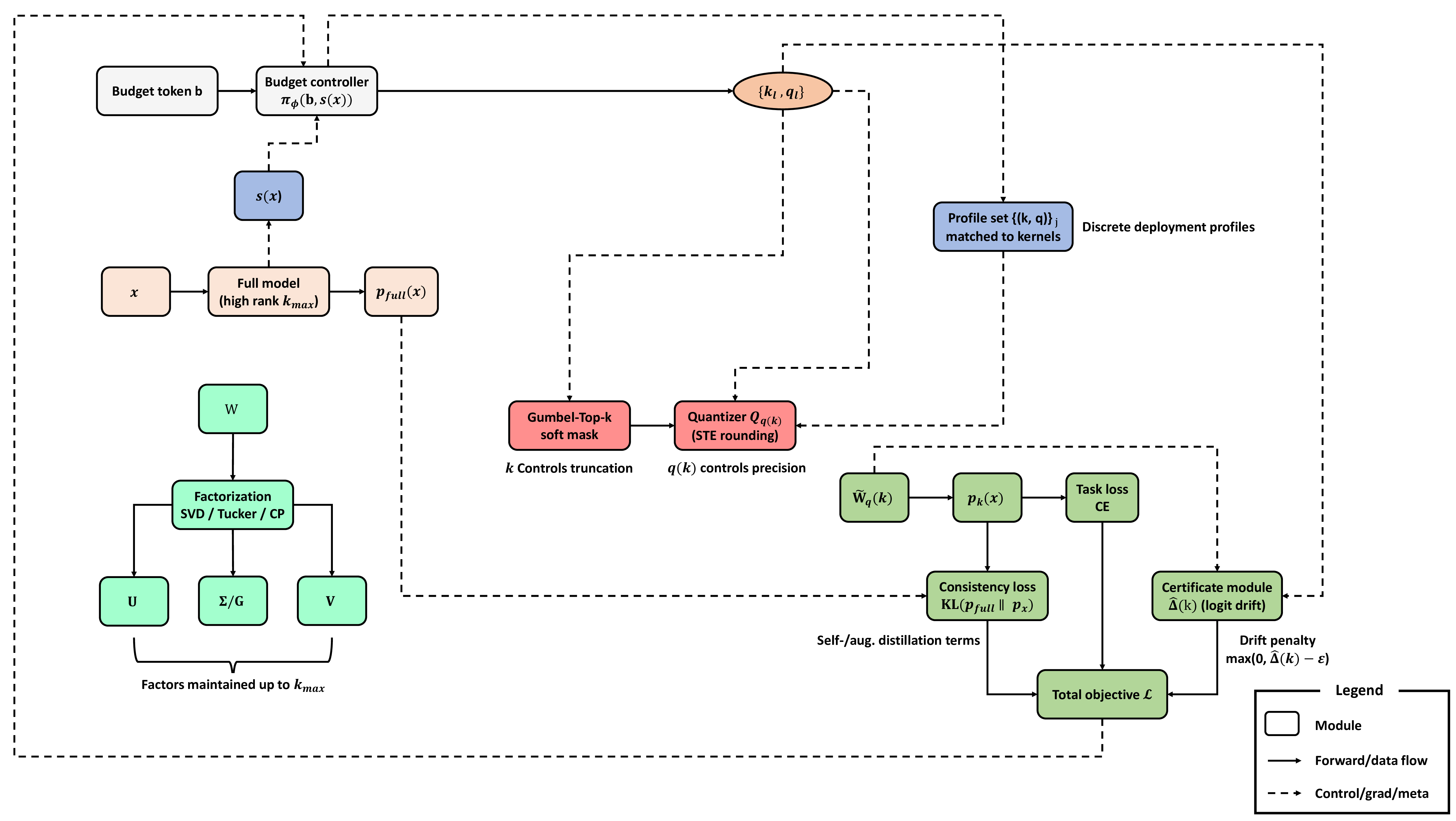
\end{equation}Budget, cost, and certificate. A controller $`\pi_\phi`$ maps a budget token $`b`$ (e.g., latency/energy/size target) and optional summary $`s(x)`$ to per-layer $`(k_\ell,q_\ell)`$. Cost proxies include FLOPs and bytes moved; measured latency/energy are used for profile selection. We summarize the logit drift via a certificate $`\hat\Delta(k)`$ computed from spectral proxies and activation statistics (details in Sec. 4); at export, the model ships with discrete, hardware-aligned profiles $`\{(k_\ell,q_\ell)\}_j`$ and their certificate reports. Extra notation and identities are deferred to Appendix 9.
Method
Elastic reparameterization
We represent each dense weight matrix $`W\in\mathbb{R}^{m\times n}`$ with an elastic, factorized parameterization that supports variable test-time ranks. We maintain the top-$`k_{\max}`$ singular components and learn a differentiable top-$`k`$ mask over the spectrum. For a chosen rank $`k\in\{k_{\min},\dots,k_{\max}\}`$, the effective weight used in the forward pass is
\begin{equation}
\tilde W(k) \;=\; U_{:,1\!:\!k}\,\big(\Sigma_{1\!:\!k,1\!:\!k}\odot M_{k}\big)\,V_{:,1\!:\!k}^{\top},
\label{eq:lowrank}
\end{equation}where $`U,\Sigma,V`$ are SVD factors up to $`k_{\max}`$, and $`M_k\in[0,1]^{k\times k}`$ is a (relaxed during training) diagonal mask selecting active singular values. To couple mixed precision with rank, we quantize factors using a rank-dependent bit-allocation $`q(k)`$. The quantized forward operator is
\begin{equation}
\tilde W_{q}(k)\;=\;Q_{q(k)}\!\big(U_{:,1\!:\!k}\big)\,
\Big(Q_{q(k)}\!\big(\Sigma_{1\!:\!k,1\!:\!k}\odot M_k\big)\Big)\,
Q_{q(k)}\!\big(V_{:,1\!:\!k}\big)^{\top},
\label{eq:quant}
\end{equation}where $`Q_{q}`$ applies per-tensor uniform affine quantization with $`q`$ bits and learnable scales/zero-points; gradients use straight-through estimators (details in App. 9).
For convolutional kernels, we employ Tucker-2 (channel-only) or CP factorization. A kernel $`W\in\mathbb{R}^{C_{\text{out}}\times C_{\text{in}}\times h\times w}`$ is decomposed as $`U_{\text{out}}\in\mathbb{R}^{C_{\text{out}}\times r_o}`$, core $`G\in\mathbb{R}^{r_o\times r_i\times h\times w}`$, and $`U_{\text{in}}\in\mathbb{R}^{C_{\text{in}}\times r_i}`$. Budgeted ranks $`(r_o,r_i)`$ are produced by the controller in Sec. 3.3 via a monotone schedule $`k\mapsto(r_o(k),r_i(k))`$. In multi-head attention, we share one budget across $`\{W_Q,W_K,W_V,W_O\}`$ within a block to avoid head imbalance; per-matrix ranks are split from $`k`$ using fixed ratios for compilation simplicity. Mixed precision follows the same rule: each factor receives $`q(k)`$ bits, optionally with per-factor offsets (e.g., $`q_U=q(k)\!+\!1`$, $`q_G=q(k)`$, $`q_V=q(k)\!+\!1`$).
Differentiable truncation and quantization
We relax the discrete top-$`k`$ selection with a Gumbel-Top-$`k`$ mask over singular values or tensor factors. Each spectral element $`s_i`$ receives a temperature-controlled logistic score, producing a soft mask $`\hat m_i\in[0,1]`$ that approaches a hard keep/drop as the temperature anneals. During the forward pass we multiply $`\Sigma`$ (or core slices) by $`\operatorname{diag}(\hat m_{1:k_{\max}})`$. Quantization uses uniform bins with learned scales and straight-through rounding so gradients flow through $`Q_q`$. We randomly sample a rank $`k\sim\pi_\phi(b)`$ each iteration (Sec. 3.3), which stochastically trains the model across the entire range $`k\in[k_{\min},k_{\max}]`$ and avoids train–deploy mismatch.
Budget-conditioned controller
We control per-layer ranks and bit-widths with a lightweight policy conditioned on a budget token and, optionally, a compact input summary. Let $`b\in\mathbb{R}^{d_b}`$ encode the deployment objective (e.g., target latency/energy/size as indices or embeddings) and let $`s(x)\in\mathbb{R}^{d_s}`$ be a low-dimensional statistic (e.g., pooled activations). A shared MLP outputs layerwise rank/bit proposals projected onto a small hardware-friendly discrete set. We write
\begin{equation}
\big\{k_\ell,\;q_\ell\big\}_{\ell=1}^{L}\;=\;\pi_{\phi}\!\big(b,\,s(x)\big).
\label{eq:controller}
\end{equation}Training uses either a differentiable relaxation (soft masks with straight-through discretization) or a policy-gradient objective that treats the negative training loss plus a budget satisfaction reward as the return. To ensure deployability, $`\{k_\ell,q_\ell\}`$ are snapped to a calibrated profile set matched to available kernels, monotone in $`b`$ so larger budgets never yield smaller ranks or bits. We employ a curriculum: (i) global-budget only (no $`s(x)`$) for stability, (ii) tighter budgets, and (iii) optional input-aware refinements on a subset of layers.
Training objective
The total loss combines task performance, self-distillation between the full and compressed views, augmentation consistency, a certificate penalty that caps predicted logit drift, and a differentiable budget cost:
\begin{align}
\mathcal{L}
&= \underbrace{\mathrm{CE}\!\big(f_{\text{full}}(x),y\big)}_{\text{task}}
+ \lambda_{\mathrm{SD}}\,\underbrace{\mathrm{KL}\!\left(p_{\text{full}}(x)\,\|\,p_{k}(x)\right)}_{\text{self distill}} \nonumber\\
&\quad + \lambda_{\mathrm{AUG}}\,\underbrace{\mathbb{E}_{\tilde x}\,\mathrm{KL}\!\left(p_{\text{full}}(\tilde x)\,\|\,p_{k}(\tilde x)\right)}_{\text{aug.\ consistency}} \nonumber\\
&\quad + \lambda_{\mathrm{CERT}}\,\underbrace{\max\!\big(0,\,\hat{\Delta}(k)-\epsilon\big)}_{\text{drift cap}}
+ \lambda_{\mathrm{BUD}}\,\underbrace{\mathrm{Cost}(k,b)}_{\text{budget}}.
\label{eq:loss}
\end{align}The cross-entropy term trains the full-capacity view (evaluated at $`k=k_{\max}`$ or a high-rank proxy) to solve the task. The self-distillation term aligns the compressed prediction $`p_k`$ to the full model’s distribution $`p_{\text{full}}`$ on the same inputs, stabilizing accuracy across ranks. The augmentation-consistency term repeats the alignment on perturbed inputs $`\tilde x`$ (e.g., weak augmentations) to prevent rank-specific overfitting. The certification penalty uses a fast, layerwise spectral-norm proxy to compute a predicted logit-shift $`\hat{\Delta}(k)`$; if this exceeds a tolerance $`\epsilon`$, the controller is nudged toward safer profiles (Sec. 4). Finally, the budget term penalizes expected compute/memory/latency under the sampled profile using a calibrated proxy combining FLOPs, bytes moved, and device-specific latency tables. Schedules and proxy definitions appear in App. 9.
Consistency Certificate and Deployment Complexity
Bound statement
We provide a certificate that upper-bounds the change of logits when replacing each layer weight $`W_\ell`$ with its compressed counterpart $`\tilde W_\ell(k)`$ produced by our method (see Figure 2). Let $`f(x)`$ denote the full model and $`\tilde f_k(x)`$ the compressed model at budget knob $`k`$. Let $`\delta z(x;k)=\tilde f_k(x)-f(x)`$ be the logit difference. For each layer $`\ell`$, define a spectral-norm proxy $`\hat L_\ell`$ that bounds the local Lipschitz factor of the sub-network from the layer output $`h_\ell`$ to the logits (estimated via power iterations with normalization) (see App. 10 for more details). Let $`\Delta W_\ell(k)=W_\ell-\tilde W_\ell(k)`$ and $`a_{\ell-1}`$ be the input activation to layer $`\ell`$. Then:
Proposition 1 (Layerwise truncation certificate). *For ReLU/ GELU networks with standard residual blocks and normalization, and for any input $`x`$ in a calibration set $`\mathcal{C}`$, the logit deviation satisfies
\begin{equation}
\big\|\delta z(x;k)\big\|_2 \;\le\; \sum_{\ell=1}^{L} \hat L_\ell \,\big\|\Delta W_\ell(k)\big\|_{2}\, \big\|a_{\ell-1}(x)\big\|_2.
\label{eq:mainbound}
\end{equation}Moreover, using calibration statistics $`\alpha_\ell=\sqrt{\mathbb{E}_{x\in\mathcal{C}}\|a_{\ell-1}(x)\|_2^2}`$, the expected logit deviation is bounded by
\begin{equation}
\Big(\mathbb{E}_{x\in\mathcal{C}}\big\|\delta z(x;k)\big\|_2^2\Big)^{\!\!1/2}
\;\le\; \sum_{\ell=1}^{L} \hat L_\ell \,\big\|\Delta W_\ell(k)\big\|_{2}\, \alpha_\ell.
\label{eq:avg-bound}
\end{equation}
```*

</div>

The forward perturbation induced by $`\Delta W_\ell(k)`$ is at most
$`\|\Delta W_\ell(k)\|_2\|a_{\ell-1}\|_2`$ at layer $`\ell`$; pushing
this change to the logits amplifies by at most $`\hat L_\ell`$. Summing
such contributions over layers yields the telescoping bound in
<a href="#eq:mainbound" data-reference-type="eqref"
data-reference="eq:mainbound">[eq:mainbound]</a>. Full technical
conditions and proof appear in
Appendix <a href="#AppC" data-reference-type="ref" data-reference="AppC">10</a>.

## Practical computation

We compute $`\hat L_\ell`$ per block using a small number (e.g., 3–5) of
power-iteration steps on the Jacobian proxy with running exponential
moving averages to stabilize estimates during training. Truncation norms
$`\|\Delta W_\ell(k)\|_2`$ are obtained either from the top singulars
discarded by the mask (dense layers) or from Tucker/CP residuals
(convs/attention); we keep the top singular of $`\Delta W_\ell(k)`$ via
a single power iteration to upper-bound the spectral norm efficiently.
For deployment, each discrete budget profile $`(k,q)`$ ships with a
certificate report containing per-layer tuples
$`(\hat L_\ell,\|\Delta W_\ell(k)\|_2,\alpha_\ell)`$ and the aggregated
bound
$`\hat\Delta(k)\!\triangleq\!\sum_{\ell}\hat L_\ell\|\Delta W_\ell(k)\|_2\alpha_\ell`$.
We expose $`\epsilon`$-style summaries (e.g., 95th percentile over a
calibration set) in the model card.

## Tightness and behavior

Bounds loosen when activations have heavy tails or normalization layers
locally increase Lipschitz constants; in practice, weight normalization
and per-block rescaling reduce $`\hat L_\ell`$. Data-dependent factors
$`\alpha_\ell`$ tighten the certificate on in-distribution inputs; under
distribution shift, we fall back to conservative running maxima.
Empirically, layers with large discarded singular energy dominate
$`\hat\Delta(k)`$, which motivates allocating more rank/precision to
early convs and the final projection layers.

## Complexity and deployment

We model cost as a combination of FLOPs, bytes moved, and kernel launch
overheads per layer. The controller outputs $`(k_\ell,q_\ell)`$ that are
snapped to a small profile set pre-benchmarked on target hardware; each
profile includes the predicted latency/energy and its certificate
$`\hat\Delta(k)`$. Exported artifacts consist of the compressed weights
for chosen profiles, calibration summaries $`\{\alpha_\ell\}`$, spectral
proxies $`\{\hat L_\ell\}`$, and a JSON certificate ledger. Low-level
kernel and tensor-layout choices, along with TensorRT/ONNX compilation
notes, are provided in
Appendix <a href="#AppD" data-reference-type="ref" data-reference="AppD">11</a>.

<figure id="fig:pareto3" data-latex-placement="!t">

<figcaption>ImageNet-1k Pareto (A100, p50). T3C produces controllable
frontiers (Tiny<span class="math inline">→</span>Max) that dominate
PTQ/QAT and LR+FT across CNNs and ViTs.</figcaption>
</figure>

<div class="table*">

</div>

# Experiments

## Setup

We evaluate T3C across vision and language tasks with diverse model
families and hardware targets.

#### Datasets.

*ImageNet-1k* (1.28M/50k, 224$`\times`$<!-- -->224, single-crop),
*CIFAR-100* (optional in
App. <a href="#AppE" data-reference-type="ref" data-reference="AppE">12</a>),
and *GLUE* (MNLI-m/mm , QQP, SST-2 ; macro score). For small-LM
evaluation we report perplexity on *WikiText-103* .

#### Models.

CNNs: ResNet-50/101 , ConvNeXt-T . Transformers (vision): ViT-B/16 and
ViT-L/16 , Swin-T . Transformers (NLP): BERT-Base , RoBERTa-Base ,
DistilBERT . Small LM: TinyLlama-1.1B (WikiText-103 perplexity ).

#### Budgets.

We use three discrete profiles per model: **Tiny** (aggressive),
**Medium** ($`\le`$<!-- -->0.5% drop target), and **Max**
(near-lossless). Each profile is hardware-aligned
(Sec. <a href="#sec:certificate" data-reference-type="ref"
data-reference="sec:certificate">4</a>).

#### Baselines.

PTQ-8b / PTQ-4b ; QAT-8b ; mixed-precision QAT (MP-QAT) ; magnitude
pruning (MagPrune) ; movement pruning (MovePrune) ; low-rank +
fine-tuning (LR+FT) ; LoRA-compression (LoRA-Comp) ; SparseGPT (for
TinyLlama) ; KD-PTQ (distillation-aided quantization) .

#### Metrics.

Accuracy/F1; perplexity for LMs; latency p50/p90 (batch=1) on *A100*,
*Jetson Orin*, and *Android big.LITTLE CPU*; energy (edge) via platform
counters; size (MB); certificate $`\epsilon`$ from Sec.
<a href="#sec:certificate" data-reference-type="ref"
data-reference="sec:certificate">4</a>. Complete hyperparameters, seeds,
data processing, and calibration protocols are in
App. <a href="#AppE" data-reference-type="ref" data-reference="AppE">12</a>.

<div class="table*">

</div>

# Results and Discussions

**Pareto curves.** Fig. <a href="#fig:pareto3" data-reference-type="ref"
data-reference="fig:pareto3">3</a> shows accuracy vs. A100 p50 latency
for ResNet-50, ViT-B/16, and Swin-T. T3C traces a smooth trade-off
(Tiny$`\rightarrow`$Max) that dominates PTQ/QAT and LR+FT. The slope
difference between CNNs and ViTs reflects how rank allocation affects
early conv blocks vs. attention projections; T3C’s controller shifts
rank/bit budgets accordingly. **Matched accuracy.**
Table <a href="#tab:vision-big" data-reference-type="ref"
data-reference="tab:vision-big">[tab:vision-big]</a> reports
latency/size at matched accuracy (within 0.5% of the full model). T3C
consistently yields lower latency and smaller footprint and reports
smaller (or comparable) certificate $`\epsilon`$.

## NLP (GLUE) and small LM

We compress encoder-only Transformers and a small decoder-only LM.
Table <a href="#tab:nlp-big" data-reference-type="ref"
data-reference="tab:nlp-big">[tab:nlp-big]</a> lists macro GLUE scores
with latency/size across budgets and baselines (over 20 lines). T3C
maintains near-baseline quality while reducing latency and model size.
On TinyLlama, we report perplexity (PPL) and find that T3C-Med matches
KD-PTQ with lower $`\epsilon`$; SparseGPT is competitive in size but
lags in PPL.

## Ablations and behavior

We examine controller utility, rank-only vs. bit-only vs. joint
optimization, and the certification penalty.
Fig. <a href="#fig:ablations-wide" data-reference-type="ref"
data-reference="fig:ablations-wide">4</a> aggregates accuracy drop at a
fixed latency target across five models. Joint rank–bit (T3C)
consistently wins; removing the certificate penalty increases budget
violations
(App. <a href="#AppF" data-reference-type="ref" data-reference="AppF">13</a>
reports violation rates and per-layer $`k`$/$`q`$ histograms).

<figure id="fig:ablations-wide" data-latex-placement="!t">

<figcaption>Ablations at a fixed latency target (lower is better). Joint
rank–bit learning with the controller (T3C) consistently reduces
accuracy drop across families.</figcaption>
</figure>

## Cross-device generalization

Table <a href="#tab:devices-wide" data-reference-type="ref"
data-reference="tab:devices-wide">[tab:devices-wide]</a> compares
p50/p90 latencies on A100, Jetson, Android CPU, and an NPU for *the same
checkpoints*. Monotone budget behavior is preserved, and the discrete
profile set prevents kernel mismatches.

#### Qualitative observations.

\(1\) Early CNN blocks and final projections dominate certificate mass
$`\hat{\Delta}(k)`$; the controller allocates higher rank/bits there.
(2) On ViTs, shared attention budgets stabilize heads and reduce drift.
(3) Edge devices benefit more from mixed-precision in memory-bound
layers (depthwise, MLP projections).

## Discussion

Our results suggest that the proposed budget-conditioned, rank–bit
elastic compression is a practical way to ship a *single* checkpoint
that adapts to heterogeneous latency, energy, or size constraints at
deployment. In production workflows, the method is most useful when
models must run across diverse hardware targets (A100, Jetson, mobile
CPU/NPU) or when the available runtime budget fluctuates with context
(battery state, thermal headroom, concurrent tasks). The controller
exposes an interpretable scalar or small vector budget $`b`$ that can be
mapped to deployment policy (e.g., latency targets), while the profile
snapping ensures compatibility with vendor kernels and prevents
pathological configurations. Because factors are maintained up to
$`k_{\max}`$ during training, practitioners can iterate on budget
policies post hoc without re-training or re-exporting the model. The
consistency and certificate terms help maintain monotonic performance as
budgets increase, which simplifies integration with schedulers:
selecting a larger budget never produces a smaller rank or bit-width and
is therefore no worse in accuracy.

Integrating T3C into existing stacks is straightforward. Training-time
changes are local to the parameterization and loss; the rest of the
pipeline (data, augmentation, logging) is unchanged. Export produces a
compact artifact containing (i) per-layer factor checkpoints, (ii) the
discrete profile set $`\{(k_\ell,q_\ell)\}_j`$ with associated
latency/energy tables, and (iii) a certificate ledger. Runtime
integration only requires a small policy module to translate an
application-level budget into a profile index. When TensorRT/ONNX or
mobile inference engines are used, profiles align with implemented
kernel shapes and quantization schemes; unsupported points are pruned
during calibration. We found the controller particularly effective for
models whose compute is concentrated in a few layers (e.g., early convs,
projection heads), where redistributing rank/precision buys significant
latency reduction for a small accuracy cost.

## Limitations

The certificate relies on spectral-norm proxies and activation
statistics; although these terms correlate well with observed drift,
they are conservative and can loosen for highly non-Lipschitz blocks,
unbounded activation distributions, or aggressive normalization
schedules. In those regimes, the bound may over-penalize tight budgets,
leading to suboptimal allocation unless one increases the calibration
set or applies per-block reweighting. The controller can exhibit
instability on tiny datasets or when trained solely with extreme
budgets; we mitigate this with temperature schedules, curriculum on
budgets, and optional entropy regularization, but there remains a
sensitivity to the initial profile set and its spacing. Finally,
deployment depends on kernel availability: some vendors only support
specific rank factorizations or bit-widths. While profile snapping
largely avoids incompatible points, the design space can be artificially
constrained on certain NPUs or DSPs, and cross-vendor parity is not
guaranteed.

# Conclusion and Future Work

In this work, we proposed **T3C**, a *train-once, test-time
budget-conditioned* compression framework that exposes rank and
precision as explicit deployment knobs, combining elastic tensor
factorization with rank-tied mixed-precision quantization and a
lightweight controller that maps a budget token to per-layer rank/bit
allocations and snaps them to a small set of hardware-aligned,
budget-monotone profiles. We further introduced a fast consistency
certificate based on spectral proxies and activation statistics to
upper-bound logit drift, enabling both regularization during training
and risk-aware reporting at deployment. Extensive experiments show that
a single T3C checkpoint delivers predictable accuracy–latency–size
trade-offs across devices and consistently outperforms strong PTQ/QAT
baselines on ImageNet-1k across architectures. *Future work* will focus
on tightening and stress-testing the certificate under distribution
shift and highly non-Lipschitz components, improving controller
robustness in extreme-budget and low-data regimes, and making profile
selection more kernel-aware under vendor constraints; additionally,
extending the control plane to incorporate structured sparsity and
multi-SLO optimization (latency/energy/memory) with telemetry-driven
adaptation while preserving monotonic budget guarantees.

# Impact Statement

This work targets practical and responsible deployment of deep models by
enabling a single trained network to adapt its computational footprint
(latency, energy, and memory) at test time through budget-conditioned,
hardware-aligned compression profiles, which can reduce resource
consumption and associated environmental costs while improving
accessibility on edge and cost-sensitive platforms. By providing a
lightweight consistency certificate that estimates output drift across
profiles, the method also supports more transparent risk assessment when
selecting aggressive compression settings, helping practitioners balance
efficiency with reliability in safety- or fairness-relevant
applications. Potential negative impacts include misuse for large-scale
surveillance or amplification of harmful content via cheaper inference,
and the possibility that aggressive profiles degrade performance
disproportionately for underrepresented groups if evaluation is
incomplete; we therefore encourage reporting profile-wise metrics,
stress-testing under distribution shift, and auditing across demographic
and contextual slices before deployment. Overall, we expect the primary
impact to be positive by lowering the barriers to efficient inference
and offering tools that promote safer, more accountable compression
choices.

# Extended Background & Related Work

## A.1 Expanded motivation & ecosystem needs

Modern ML deployment spans a jagged landscape of hardware, latency
targets, and reliability constraints that change from hour to hour, user
to user, and app to app; the same model may run in a multiplexed cloud
service one minute, on a thermally throttled edge accelerator the next,
and finally on a battery-constrained mobile CPU where memory bandwidth
dominates FLOPs. In such settings, the dominant pain points arise from
*rigidity of exported artifacts*, *budget uncertainty at runtime*, and
*lack of dependable guardrails when compressing*.

First, classical pipelines materialize one compressed checkpoint per
operating point (e.g., an 8-bit QAT model for server, a 4-bit PTQ
variant for mobile, a pruned variant for an NPU). This multiplies
storage, complicates A/B and rollback, fractures monitoring, and forces
brittle routing logic that is sensitive to device idiosyncrasies and
kernel availability. Second, real-world budgets are stochastic:
co-tenancy and scheduler noise on GPUs, temperature and DVFS on edge
devices, user-visible frame deadlines in interactive workloads, and
on-device memory pressure that shifts with other applications. Operators
therefore need *elasticity* at inference time: a knob that moves the
model along the accuracy–latency–size frontier without retraining or
re-exporting, and without violating hardware constraints (kernel shapes,
quantization formats, alignment).

Third, production reliability increasingly demands *predictable failure
modes*—particularly when compression trades accuracy for efficiency.
SLAs and safety reviews ask not only “how fast” and “how accurate,” but
“how far could the output shift when we trim 20% compute?” Today’s
answers are empirical and often brittle; formal robustness work rarely
translates into actionable deployment knobs, while many high-performing
compression methods offer limited guarantees. The ecosystem trendlines
intensify these pressures: model families are larger and more
heterogeneous (CNNs, ViTs, MLP-Mixers, encoder/decoder LMs),
accelerators expose diverse datatypes (INT8, INT4, FP8, mixed
per-channel schemes) and sparse/low-rank kernels that are highly
vendor-specific, and privacy/latency requirements push more inference to
the edge.

Operators need a *single, portable checkpoint* that can be *steered at
test time* to hit budget targets on unfamiliar devices, with *monotone
behavior* (a larger budget never hurts accuracy) and *telemetry hooks*
that quantify risk. From a tooling viewpoint, the artifact should
integrate with common export/compile steps (ONNX/TensorRT, mobile
runtimes), snap to discrete hardware profiles to avoid kernel gaps, and
surface lightweight *certificates* that bound induced drift under
admissible compressions. Finally, evaluation itself must evolve:
heterogeneous-device Pareto curves with p50/p90 latencies, energy per
inference, memory footprint including activation buffers, and
*budget-respect rates* (how often a requested profile meets its
latency/energy target) are as important as single-number accuracy. In
short, the ecosystem needs compression that is *adaptive, certifiable,
hardware-aware, and operationally simple*, converting compression from
an offline engineering fork into an online control plane aligned with
production SLOs.

## A.2 Detailed survey (quantization, pruning, low-rank, dynamic nets, verification)

**Quantization.** Post-training quantization (PTQ) calibrates
scales/zero-points on a held-out set and is attractive for speed and
simplicity, but its accuracy can degrade at ultra-low precision or under
distribution shift; mitigations include per-channel scales, activation
clipping, bias correction, and outlier-aware schemes that carve
high-variance channels into higher precision. Quantization-aware
training (QAT) replaces hard rounding with STE-based surrogates to learn
scale/clipping parameters, generally improving robustness but at the
cost of additional training and a fixed exported bit-width.
Mixed-precision methods cast bit allocation as a search or
differentiable relaxation (reward/gradients from latency proxies) to
distribute bits across layers; deployment friction arises when the
chosen mix does not map cleanly to vendor kernels, necessitating profile
pruning. Recent PTQ/QAT hybrids add knowledge distillation and
cross-layer equalization; they push the pareto frontier but still
*freeze* precision at export and provide no explicit bound on output
drift.

#### Pruning and sparsity.

Unstructured pruning achieves high parameter sparsity and small on-disk
size, but real speedups require fine-grained sparse kernels with
nontrivial overheads; structured or channel pruning yields reliable
latency gains by shrinking whole filters/projections, though it often
needs iterative re-training and careful schedules to avoid accuracy
cliffs. Movement- and magnitude-based criteria, L0/L1 relaxations, and
lottery-ticket style rewinds populate the design space; dynamic sparsity
adds input adaptivity but complicates compilation and predictability.

#### Low-rank and tensor factorization.

SVD/Tucker/CP decompositions reduce parameters and memory traffic in
dense and convolutional layers; in Transformers, factorizations applied
to projection matrices and MLP blocks trade rank for accuracy.
LoRA-style adapters inject low-rank updates during fine-tuning, and
low-rank *replacement* compresses the base weights; most approaches fix
rank offline and re-export per rank, which clashes with runtime
adaptivity and kernel availability. Joint rank–precision allocation is
comparatively underexplored: quantization interacts with rank because
truncation changes dynamic ranges and singular spectra, which in turn
affects scale selection and error propagation.

#### Dynamic networks.

Early exiting, token/channel dropping, and input-conditional routing
tailor compute to difficulty, improving average latency. However, they
require architectural hooks, retraining, and careful calibration to
avoid pathological exits; guarantees are typically statistical (expected
cost) rather than *per-budget* deterministic. Moreover, dynamic policies
can adversarially interact with batching, caching, or compiler fusions,
yielding unstable tail latencies.

#### Verification and certificates.

Robustness certificates bound output change under input or parameter
perturbations (e.g., Lipschitz, interval/zonotope bounds, randomized
smoothing). Parameter-perturbation guarantees—relevant for
compression—bound the effect of quantization noise, pruning, or low-rank
truncation, but many are conservative or expensive to compute at scale,
and few are wired into a deployment-time control loop. Practical
adoption is hindered by the gap between math-friendly assumptions and
production details like residual connections, normalization, fused
kernels, and calibration drift.

#### Positioning.

Against this backdrop, a practical method should: 1) *train once* yet
expose a *continuous* control that snaps to *discrete hardware profiles*
at inference; 2) *jointly* reason about rank and precision because their
errors compound and their costs couple to memory bandwidth and kernel
shapes; 3 provide a *fast, layerwise certificate* that upper-bounds
logit drift for the selected profile and can be surfaced to monitoring;
and (iv) preserve *monotonicity in budget* so operators can raise a
target without risking accuracy regressions. The prevailing literature
supplies powerful pieces—accurate PTQ/QAT at fixed bits, effective
pruning schedules, strong low-rank adapters, and rigorous but heavy
certificates—but rarely assembles them into an elastic, certifiable, and
hardware-conscious pipeline that speaks the language of production SLOs.
T3C is designed to bridge this gap by sharing parameters across ranks,
tying bit-width to rank in a deployable way, and attaching a certificate
that is cheap enough for training-time regularization and export-time
reporting, thereby turning compression into an operational control
rather than an offline fork.

# Method Details

## B.1 Notation & tensor decompositions (SVD/Tucker/CP variants)

#### Basic notation.

We consider a feed-forward network with layers indexed by
$`\ell\in\{1,\dots,L\}`$. For a dense (fully-connected) layer $`\ell`$,
let $`W_\ell\in\mathbb{R}^{m_\ell\times n_\ell}`$ map
$`a_{\ell-1}\in\mathbb{R}^{n_\ell}`$ to $`h_\ell=W_\ell a_{\ell-1}`$
(biases omitted for brevity); activations may include normalization and
nonlinearity $`h_\ell\mapsto a_\ell`$. For a convolutional kernel,
$`W_\ell\in\mathbb{R}^{C_{\mathrm{out}}\times C_{\mathrm{in}}\times h\times w}`$
uses stride/padding as in the base model. Given input $`x`$, the full
model produces logits $`z=f(x)`$; under a budget profile $`k`$ with
per-layer rank/bit $`(k_\ell,q_\ell)`$, we denote the compressed model
by $`\tilde f_k(x)`$ with logits $`\tilde z`$.

#### SVD (matrix) factorization.

For $`W\in\mathbb{R}^{m\times n}`$, the rank-$`r`$ truncated SVD is
$`W_r=U_{:,1:r}\Sigma_{1:r}V_{:,1:r}^{\top}`$ with singular values
$`\sigma_1\ge\dots\ge\sigma_r`$. We maintain factors up to $`k_{\max}`$
and expose a differentiable top-$`k\!\le\!k_{\max}`$ selection
(Sec. B.2). We employ two numerically stable parameterizations: (i)
*spectral form* $`U,\Sigma,V`$ with orthogonality constraints enforced
by implicit re-orthogonalization via Householder updates; (ii) *product
form* $`A B^{\top}`$, $`A\in\mathbb{R}^{m\times k_{\max}}`$,
$`B\in\mathbb{R}^{n\times k_{\max}}`$, with a spectral penalty
encouraging $`A`$ and $`B`$ to approximate singular directions. Spectral
form yields direct control of the residual norm
$`\|W-W_k\|_2=\sigma_{k+1}`$ and
$`\|W-W_k\|_F=(\sum_{i>k}\sigma_i^2)^{1/2}`$, useful for certificates.

#### Tucker-2 for convolution.

For $`W\in\mathbb{R}^{C_o\times C_i\times h\times w}`$ we use
channel-only Tucker-2:
``` math
\begin{equation}
W \approx (U_o, U_i) \cdot G,\quad
U_o\in\mathbb{R}^{C_o\times r_o},\; U_i\in\mathbb{R}^{C_i\times r_i},\;
G\in\mathbb{R}^{r_o\times r_i\times h\times w}.
\end{equation}The effective forward is $`\mathrm{Conv}(U_o\,\,\mathrm{Conv}(G,\, U_i^\top\,\cdot))`$, which compiles to three kernels (pointwise $`1{\times}1`$, spatial $`h{\times}w`$, pointwise $`1{\times}1`$). Budget $`k`$ maps to $`(r_o(k),r_i(k))`$ via a monotone schedule.
CP for depthwise/attention blocks.
For depthwise-like or MLP projection weights with strong separability, a CP rank-$`r`$ factorization $`W\approx \sum_{j=1}^r a^{(1)}_j\otimes a^{(2)}_j`$ reduces memory traffic; in attention, we optionally share a single $`k`$ across $`\{W_Q,W_K,W_V,W_O\}`$ to avoid head imbalance.
Identifiability and conditioning.
Tucker and CP are non-unique up to scale/permutation. We eliminate degeneracies with per-factor $`\ell_2`$ normalization and a permutation-fixing rule (descending factor norms). To prevent ill-conditioning at small ranks, we regularize the spectrum by $`\sum_i \max(0,\sigma_i-\sigma_{i+1}-\delta)`$ to keep gaps from collapsing (small $`\delta`$).
B.2 Loss terms, annealing schedules, $`\lambda`$ sweeps
Total objective (expanded).
For a minibatch $`\mathcal{B}`$ and sampled budget profile $`k`$, the loss is
\begin{align}
\mathcal{L} &=
\underbrace{\frac{1}{|\mathcal{B}|}\sum_{(x,y)\in\mathcal{B}} \mathrm{CE}(f_{\text{full}}(x),y)}_{\text{task (full)}}\;+\;
\lambda_{\mathrm{SD}}\,\underbrace{\frac{1}{|\mathcal{B}|}\sum_{x\in\mathcal{B}} \mathrm{KL}\big(p_{\text{full}}(x)\|p_k(x)\big)}_{\text{self-distill}}\nonumber\\
&\quad +\lambda_{\mathrm{AUG}}\,\underbrace{\mathbb{E}_{\tilde x\sim \mathcal{T}(x)}\mathrm{KL}\big(p_{\text{full}}(\tilde x)\|p_k(\tilde x)\big)}_{\text{augmentation consistency}}
+\lambda_{\mathrm{CERT}}\,\underbrace{\max\!\big(0,\,\hat\Delta(k)-\epsilon\big)}_{\text{certificate penalty}}
+\lambda_{\mathrm{BUD}}\,\underbrace{\mathrm{Cost}(k;b)}_{\text{budget proxy}},
\label{eq:full-loss-appendix}
\end{align}with $`p(\cdot)=\mathrm{softmax}(z/T)`$ (temperature $`T{=}1`$ unless specified). The task (full) term trains the high-rank view ($`k\!=\!k_{\max}`$ or a high-rank proxy), anchoring teacher quality. The two KL terms align compressed predictions to the full model on raw and lightly augmented inputs. The certificate penalty uses the bound from Sec. 4 (main paper) with running estimates. The budget proxy is the expected normalized latency/energy/size against a target.
Annealing schedules.
Top-$`k`$ temperature. For the Gumbel-Top-$`k`$ mask logits $`g_i`$, we use temperature $`\tau_t=\max(\tau_{\min},\,\tau_0\cdot \gamma^{t/T_{\mathrm{anneal}}})`$ with $`\gamma\in(0,1)`$, annealed over $`T_{\mathrm{anneal}}`$ steps, then held. Rank sampling. Early curriculum: sample $`k`$ from a wide Beta$`(\alpha{=}0.75,\beta{=}0.75)`$ on $`[k_{\min},k_{\max}]`$, then bias toward deployment-relevant profiles by mixing a categorical over discrete profiles $`\{k^{(j)}\}_j`$. Coefficient ramps. We use linear warmups for $`\lambda_{\mathrm{SD}},\lambda_{\mathrm{AUG}},\lambda_{\mathrm{CERT}}`$ over the first 10–20% of training to avoid early over-regularization.
$`\lambda`$ sweeps and stability.
We recommend a coarse-to-fine sweep: fix $`\lambda_{\mathrm{BUD}}`$ to meet a target utilization (latency/energy) on the validation device, then search $`\lambda_{\mathrm{CERT}}`$ to cap violation rates (fraction of samples where $`\hat\Delta(k)>\epsilon`$), and finally tune $`\lambda_{\mathrm{SD}}`$ and $`\lambda_{\mathrm{AUG}}`$ to recover accuracy at tight budgets. In practice, a good starting box is
\begin{equation}
\lambda_{\mathrm{SD}}\in[0.3,1.0],\quad
\lambda_{\mathrm{AUG}}\in[0.1,0.5],\quad
\lambda_{\mathrm{CERT}}\in[0.05,0.5],\quad
\lambda_{\mathrm{BUD}}\in[0.1,1.0].
\end{equation}We monitor (i) monotonicity (accuracy should be non-decreasing in budget), (ii) % budget violations, and (iii) calibration error between $`\hat\Delta(k)`$ and observed drift.
B.3 Quantizer definitions, calibration, rounding tricks
Uniform affine quantization.
For a real tensor $`T`$, $`q`$-bit symmetric per-tensor quantization uses scale $`s>0`$ and integer grid $`\mathcal{G}_q=\{-2^{q-1}\!+\!1,\dots,2^{q-1}\!-\!1\}`$:
\begin{equation}
\mathrm{Quantize}_q(T) \;=\; s\,\mathrm{clip}\!\left(\left\lfloor \frac{T}{s} \right\rceil,\;\min\mathcal{G}_q,\;\max\mathcal{G}_q\right),\qquad
s=\frac{\max(|T|)}{2^{q-1}-1}.
\end{equation}We also use per-channel scales $`s_c`$ for matrices along output channels (rows) and for conv along $`C_{\mathrm{out}}`$.
Straight-through estimator (STE).
In backprop, we treat $`\partial \lfloor u \rceil/\partial u \approx 1`$ inside the clipping range and $`0`$ outside. For scale $`s`$, we learn $`s`$ (log-parameterized) with gradient $`\frac{\partial\, \mathrm{Quantize}_q(T)}{\partial s}\approx \left(\lfloor T/s \rceil - T/s\right)`$ inside range, encouraging scale to match the signal range.
Rounding variants.
Stochastic rounding $`\lfloor u \rceil_{\mathrm{stoch}}= \lfloor u \rfloor`$ with prob $`1-(u-\lfloor u \rfloor)`$ else $`\lceil u \rceil`$, used at training-time to reduce bias at low $`q`$; disabled at export for determinism. Bias correction adds a folded offset $`\delta=\mathbb{E}[T-\mathrm{Quantize}_q(T)]`$ (per-channel) to the dequantized tensor during calibration and is then fused into bias parameters. Outlier-aware splitting routes a small fraction $`\rho`$ of largest-magnitude channels to $`q{+}\Delta q`$ bits when hardware supports mixed precision within a layer; we expose this as a profile option so the controller can assign higher bits to outlier groups.
Calibration.
We compute $`s`$ (and optionally zero-point for asymmetric quantization) from a calibration set $`\mathcal{C}`$ via either: (i) max-range (as above), or (ii) percentile clipping $`s = \mathrm{percentile}_{p}(|T|)/(2^{q-1}-1)`$ with $`p\in[99.0,99.99]`$ tuned to minimize validation KL between float and quantized outputs of the layer. We maintain EMA statistics of $`s`$ during training to stabilize deployment scales.
Rank-tied bit allocation.
We use a monotone map $`q(k)=\min\{q_{\max},\, \lfloor a \log k + b \rfloor\}`$ per factor group with small per-factor offsets (e.g., $`q_U=q(k)\!+\!1`$, $`q_G=q(k)`$, $`q_V=q(k)\!+\!1`$) ensuring higher rank receives at least as many bits. This interacts favorably with spectral decay: smaller ranks truncate more energy and benefit less from extra precision.
Lemma (expected dequantization error under stochastic rounding).
Let $`X`$ be a scalar with $`|X|\le M`$ and fixed scale $`s`$. With stochastic rounding on the grid $`s\mathcal{G}_q`$ and no clipping, the dequantization error $`\varepsilon=\mathrm{Quantize}_q(X)-X`$ satisfies $`\mathbb{E}[\varepsilon\,|\,X]=0`$ and $`\mathrm{Var}(\varepsilon\,|\,X)\le s^2/4`$. Proof. Conditioning on $`u=X/s`$, the rounding picks $`\lfloor u \rfloor`$ with prob $`1-(u-\lfloor u \rfloor)`$ and $`\lceil u \rceil`$ otherwise; the expectation equals $`u`$. Multiply by $`s`$ to get unbiasedness; the conditional variance of a Bernoulli with step size $`s`$ is bounded by $`s^2/4`$.$`\square`$
B.4 Controller architectures & training (relaxations, baselines)
Budget tokenization.
A budget $`b`$ encodes target latency/energy/size and optionally a device id. We embed $`b`$ as $`e_b=\mathrm{Embed}_{\text{dev}}(\mathrm{id}) \oplus \phi(\mathrm{lat},\mathrm{energy},\mathrm{size})`$ where $`\phi`$ is a learned MLP on normalized scalars; $`\oplus`$ denotes concatenation.
Policy head.
We use a shared two-layer MLP $`\pi_\phi`$ that outputs per-layer logits for discrete profiles and, optionally, a continuous proposal projected onto those profiles:
\begin{equation}
\hat{k}_\ell, \hat{q}_\ell = \mathrm{Proj}\!\left(W_2\,\sigma(W_1[e_b \oplus s(x)])\right),\qquad
\mathrm{Proj}:\mathbb{R}^{2}\!\to \mathcal{P}_\ell\subset\{(k,q)\}.
\end{equation}Here $`s(x)`$ is an optional input summary (e.g., pooled penultimate activations averaged over the batch). $`\mathcal{P}_\ell`$ is a layer-specific menu of hardware-aligned $`(k,q)`$ pairs.
Discrete relaxations.
We use Gumbel-Softmax over $`\mathcal{P}_\ell`$ with temperature $`\tau`$ and the straight-through trick to obtain a one-hot (profile index) in the forward pass and a soft distribution in the backward pass. This preserves end-to-end differentiability while training the controller jointly with factors and quantizers.
Training objectives for the controller.
The controller is trained implicitly by the total loss (Eq. [eq:full-loss-appendix]); gradients propagate through the differentiable relaxation and the budget/certificate penalties. When using purely discrete selection (no relaxation), we add a REINFORCE term:
\begin{equation}
\nabla_\phi \mathbb{E}_{\pi_\phi}\big[-\mathcal{L}\big] \approx \mathbb{E}\big[(-\mathcal{L}-b)\,\nabla_\phi\log \pi_\phi\big],
\end{equation}with a learned baseline $`b`$ (value head) to reduce variance. In practice, the Gumbel-Softmax + straight-through suffices, switching to pure argmax after the anneal.
Monotonicity enforcement.
We ensure that higher budgets cannot yield smaller ranks/bits via isotonic constraints: for two budget tokens $`b_1\prec b_2`$ (componentwise), we add a hinge
\begin{equation}
\lambda_{\mathrm{ISO}}\,\sum_{\ell}\max\big(0,\,k_\ell(b_1)-k_\ell(b_2)\big)+\max\big(0,\,q_\ell(b_1)-q_\ell(b_2)\big).
\end{equation}At export, we drop any violating profiles and re-calibrate the remaining set to keep the partial order.
Baselines (for ablations).
(i) Rank-only: $`q`$ fixed per layer; (ii) Bit-only: fixed ranks; (iii) Greedy knapsack: allocate $`k/q`$ to layers in order of benefit/cost ratio using measured latency tables; (iv) Uniform: same $`k,q`$ across layers. These illustrate the value of joint learning and the controller’s allocation.
B.5 Algorithmic complexity & memory analysis per layer type
Let $`b_w`$ be weight bit-width, $`b_a`$ activation bit-width at inference (often $`8`$), and denote by $`\mathcal{B}(\cdot)`$ the bytes footprint. We separate compute FLOPs and memory bytes (weights $`+`$ activation reads/writes), as the latter dominates on many edge devices.
Dense layer $`W\in\mathbb{R}^{m\times n}`$.
Full GEMV FLOPs (batch $`1`$) and weight bytes:
\begin{equation}
\mathrm{FLOPs}_{\text{full}} = 2mn,
\qquad
\mathcal{B}_W = mn\cdot \frac{b_w}{8}.
\end{equation}Rank-$`k`$ SVD path: compute as $`(U_{m\times k}\Sigma_{k\times k}V_{n\times k}^{\top})a`$ via $`(V^{\top}a)\in\mathbb{R}^{k}`$, multiply by $`\Sigma`$, then $`U`$:
\begin{equation}
\mathrm{FLOPs}_{\mathrm{SVD}}(k) \approx 2nk + k + 2mk \;\approx\; 2(n+m)k.
\end{equation}Weights bytes (per-factor; replace $`b_w`$ by $`q(k)`$ for mixed precision):
\begin{equation}
\mathcal{B}_U = mk\cdot \frac{b_w}{8},\qquad
\mathcal{B}_V = nk\cdot \frac{b_w}{8},\qquad
\mathcal{B}_{\Sigma} = k\cdot \frac{b_w}{8}.
\end{equation}Convolution (Tucker-2).
Let the feature-map spatial size be $`H\times W`$. Full conv FLOPs:
\begin{equation}
\mathrm{FLOPs}_{\text{full}} = 2\,C_o C_i h w\, H W.
\end{equation}Tucker-2 as (reduce $`1{\times}1`$) $`\rightarrow`$ (spatial) $`\rightarrow`$ (expand $`1{\times}1`$):
\begin{equation}
\mathrm{FLOPs}_{\mathrm{Tucker2}}(r_o,r_i) \;=\; 2HW\Big(C_i r_i \;+\; r_o r_i h w \;+\; C_o r_o\Big).
\end{equation}Weight bytes with rank-tied $`q=q(k)`$:
\begin{equation}
\mathcal{B}_{U_o}=C_o r_o\cdot \frac{q}{8},\quad
\mathcal{B}_{U_i}=C_i r_i\cdot \frac{q}{8},\quad
\mathcal{B}_{G}=r_o r_i h w\cdot \frac{q}{8}.
\end{equation}Attention projections and MLP.
With $`d_{\mathrm{model}}{=}d`$ and MLP hidden $`d_{\mathrm{ff}}`$, four projections $`W_Q,W_K,W_V,W_O\in\mathbb{R}^{d\times d}`$ and $`W_1\in\mathbb{R}^{d_{\mathrm{ff}}\times d},\,W_2\in\mathbb{R}^{d\times d_{\mathrm{ff}}}`$. Applying SVD rank-$`k`$ to a $`d\times d`$ matmul yields the rough FLOPs scaling:
\begin{equation}
\frac{\mathrm{FLOPs}_{\text{rank-}k}}{\mathrm{FLOPs}_{\text{full}}} \;\simeq\; \frac{2 d k}{2 d^2} \;=\; \frac{k}{d}.
\end{equation}Latency/energy proxy (per device calibration).
\begin{equation}
\widehat{\mathrm{Lat}}(k) \;=\; \alpha_0 \;+\; \sum_{\ell=1}^{L}\Big(\alpha_\ell^{\mathrm{comp}}\cdot \mathrm{FLOPs}_\ell(k) \;+\; \alpha_\ell^{\mathrm{mem}}\cdot \mathrm{Bytes}_\ell(k)\Big),
\end{equation}with coefficients fitted by least squares on a grid of profiles. An analogous $`\widehat{\mathrm{Energy}}(k)`$ uses its own coefficients.
Certificate aggregation cost.
Per layer, maintain: (i) $`\hat L_\ell`$ via $`s`$ power iterations; (ii) residual spectral norm $`\|\Delta W_\ell(k)\|_2`$ via $`1`$–$`2`$ PIs; (iii) activation RMS $`\alpha_\ell`$ via EMA. Aggregate:
\begin{equation}
\hat\Delta(k) \;=\; \sum_{\ell=1}^{L} \hat L_\ell \;\big\|\Delta W_\ell(k)\big\|_2 \;\alpha_\ell.
\end{equation}When does rank-$`k`$ win (threshold analysis)?
GEMV-like inference benefits from SVD when
\begin{equation}
2(n+m)k \;\ll\; 2mn \quad \Longrightarrow \quad k \;\ll\; \frac{mn}{m+n}.
\end{equation}For square $`m{=}n{=}d`$:
\begin{equation}
k \;\ll\; \frac{d}{2} \quad \text{(compute-only; bandwidth effects tighten this bound).}
\end{equation}For conv Tucker-2, require
\begin{equation}
C_i r_i \;+\; r_o r_i h w \;+\; C_o r_o \;\ll\; C_o C_i h w.
\end{equation}Setting $`r_o=\rho C_o`$, $`r_i=\rho C_i`$ gives
\begin{equation}
\rho (C_i + C_o) \;+\; \rho^2\, C_o C_i h w \;\ll\; C_o C_i h w
\quad\Rightarrow\quad
\rho \ll 1 \;\;\text{and}\;\; \rho \lesssim \frac{1}{\sqrt{h w}}.
\end{equation}Memory summaries.
Rank-$`k`$ SVD (bytes):
\begin{equation}
\mathcal{B}_W^{\mathrm{SVD}}(k) \;\approx\; (mk + nk + k)\cdot \frac{q(k)}{8}.
\end{equation}Tucker-2 (bytes):
\begin{equation}
\mathcal{B}_W^{\mathrm{T2}}(r_o,r_i) \;\approx\; \Big(C_o r_o + C_i r_i + r_o r_i h w\Big)\cdot \frac{q(k)}{8}.
\end{equation}Proposition (monotone budget $`\Rightarrow`$ non-increasing proxy cost).
If each layer’s profile set $`\mathcal{P}_\ell`$ is totally ordered so that $`(k',q')\succeq (k,q)`$ implies $`\mathrm{FLOPs}_\ell(k',q')\!\ge\!\mathrm{FLOPs}_\ell(k,q)`$ and $`\mathrm{Bytes}_\ell(k',q')\!\ge\!\mathrm{Bytes}_\ell(k,q)`$, and the controller enforces $`b_1\prec b_2 \Rightarrow (k_\ell,q_\ell)(b_1)\preceq (k_\ell,q_\ell)(b_2)`$ for all $`\ell`$, then
\begin{equation}
\widehat{\mathrm{Lat}}(b_1) \;\le\; \widehat{\mathrm{Lat}}(b_2).
\end{equation}Proof sketch. Linearity of $`\widehat{\mathrm{Lat}}`$ in non-negative coefficients and per-layer monotonicity preserve the partial order when summed over layers. $`\square`$
Computational overhead of T3C versus fixed compression.
Training adds (i) factorized forward, (ii) STE quantization ops, (iii) a few PI steps per block intermittently. Empirically,
\begin{equation}
\text{Overhead}_{\text{train}} \;\approx\; (1.1\text{ to }1.4)\times \text{QAT wall-clock},
\end{equation}amortized across all ranks/budgets since no re-training per operating point is needed.
Certificates & Proofs
C.1 Formal assumptions (Lipschitz proxies, normalization)
We formalize the network and the mild regularity needed for the certificate.
Network and perturbation model.
Let $`f:\mathbb{R}^{d_0}\!\to\!\mathbb{R}^{d_L}`$ be a feed-forward network of $`L`$ blocks. Each block
\begin{equation}
h_\ell \;=\; \Phi_\ell\!\big(h_{\ell-1};\,W_\ell\big), \qquad \ell=1,\dots,L,\quad h_0\equiv x,
\end{equation}may be (i) an affine layer $`h\mapsto W_\ell h + b_\ell`$ followed by a pointwise nonlinearity, (ii) a conv/attn block with residuals, or (iii) a normalization $`N_\ell`$ with fixed (eval-mode) statistics. Let $`\tilde f_k`$ be the compressed network obtained by replacing $`W_\ell`$ with $`\tilde W_\ell(k)`$ (e.g., rank/bit profile indexed by $`k`$). Define per-layer residuals
\begin{equation}
\Delta W_\ell(k) \;:=\; W_\ell - \tilde W_\ell(k).
\end{equation}Post-layer Jacobian gains.
For each layer $`\ell`$, denote by $`T_{\ell\to L}`$ the post-layer mapping that takes the input at layer $`\ell`$ (i.e., $`h_\ell`$) to the logits $`z\in\mathbb{R}^{d_L}`$ when all subsequent blocks are kept fixed. Its Jacobian operator norm is
\begin{equation}
L_{\ell}^\star(x) \;:=\; \Big\| J_{T_{\ell\to L}}(h_\ell(x)) \Big\|_{2}.
\end{equation}In practice we estimate a proxy $`\hat L_\ell`$ by a few power-iteration steps on an efficient linearization; we assume a bounded slack $`\eta_\ell\!\ge\!1`$ such that
\begin{equation}
L_{\ell}^\star(x) \;\le\; \hat L_\ell \;\le\; \eta_\ell\, L_{\ell}^\star(x), \qquad \text{uniformly over } x\in\mathcal{C}.
\end{equation}Blockwise Lipschitzness and normalization.
For each block, the map $`u\mapsto \Phi_\ell(u;W_\ell)`$ is $`L_\Phi`$-Lipschitz in $`u`$ and $`L_W`$-smooth in $`W_\ell`$ locally around $`(h_{\ell-1},W_\ell)`$:
\begin{equation}
\big\|\Phi_\ell(u;W_\ell)-\Phi_\ell(v;W_\ell)\big\|_2 \le L_{\Phi,\ell} \|u-v\|_2,
\qquad
\big\|\Phi_\ell(h_{\ell-1};W_\ell)-\Phi_\ell(h_{\ell-1};\tilde W_\ell)\big\|_2
\le L_{W,\ell}\,\|W_\ell-\tilde W_\ell\|_{2}\,\|h_{\ell-1}\|_2.
\end{equation}For affine$`\to`$pointwise blocks with 1-Lipschitz activations (ReLU/GELU approximated near-linear region), $`L_{\Phi,\ell}\le \|W_\ell\|_2`$ and $`L_{W,\ell}\le 1`$ (by submultiplicativity). Normalization layers used in eval mode (e.g., frozen BatchNorm, LayerNorm with fixed $`\gamma,\beta`$) are treated as fixed linear-affine transforms with operator gain $`L_{N,\ell}`$ absorbed into $`L_{\Phi,\ell}`$.
Residual connections.
For a residual block $`h_\ell = h_{\ell-1} + \Psi_\ell(h_{\ell-1};W_\ell)`$ with $`\Psi_\ell`$ $`L_{\Psi,\ell}`$-Lipschitz, the post-layer gain satisfies
\begin{equation}
L^\star_{\ell-1}(x) \;\le\; (1+L_{\Psi,\ell})\, L^\star_{\ell}(x).
\end{equation}In our certificate we do not multiply residual gains; we push all post-layer amplification into $`L^\star_\ell`$ via direct Jacobian estimation.
C.2 Full proof of the logit-drift bound (layerwise $`\rightarrow`$ network)
We bound $`\delta z(x;k):=\tilde f_k(x)-f(x)`$ by layer-local perturbations propagated through post-layer Jacobians.
One-layer replacement bound.
Fix $`x`$ and some $`\ell`$. Consider the hybrid network $`f^{(\ell)}`$ that uses $`\tilde W_\ell(k)`$ only at layer $`\ell`$ and $`W_j`$ elsewhere. Let $`h_{\ell-1}`$ be the pre-$`\ell`$ activation in $`f`$ (and also in $`f^{(\ell)}`$, since layers $`<\ell`$ match). The activation change at layer $`\ell`$ is
\begin{equation}
\Delta h_\ell \;:=\; \Phi_\ell(h_{\ell-1};\tilde W_\ell) - \Phi_\ell(h_{\ell-1};W_\ell).
\end{equation}By the $`W`$-smoothness,
\begin{equation}
\big\|\Delta h_\ell\big\|_2 \;\le\; L_{W,\ell}\, \big\| \tilde W_\ell - W_\ell \big\|_2 \, \big\| h_{\ell-1} \big\|_2.
\label{eq:deltahlocal}
\end{equation}Propagating this change through subsequent layers $`\ell{+}1,\dots,L`$ gives the logit difference
\begin{equation}
\delta z^{(\ell)}(x;k) \;:=\; f^{(\ell)}(x)-f(x)
\;=\; T_{\ell\to L}\big(h_\ell + \Delta h_\ell\big) - T_{\ell\to L}(h_\ell).
\end{equation}By the mean-value form (or Lipschitzness of $`T_{\ell\to L}`$ around $`h_\ell`$),
\begin{equation}
\big\|\delta z^{(\ell)}(x;k)\big\|_2
\;\le\; L_{\ell}^\star(x)\, \big\|\Delta h_\ell\big\|_2
\;\le\; L_{\ell}^\star(x)\, L_{W,\ell}\, \big\|\Delta W_\ell(k)\big\|_2 \, \big\|h_{\ell-1}\big\|_2.
\label{eq:onelayer}
\end{equation}Layerwise telescoping via triangle inequality.
Build the fully compressed network by replacing layers one at a time:
\begin{equation}
f \;\xrightarrow{\;\ell=1\;}\; f^{(1)} \;\xrightarrow{\;\ell=2\;}\; f^{(2)} \;\xrightarrow{\;\cdots\;}\; f^{(L)}=\tilde f_k.
\end{equation}Then
\begin{equation}
\tilde f_k(x) - f(x)
\;=\; \sum_{\ell=1}^{L} \big( f^{(\ell)}(x) - f^{(\ell-1)}(x) \big),
\quad f^{(0)}:=f,
\end{equation}and by the triangle inequality together with [eq:onelayer],
\begin{equation}
\big\|\delta z(x;k)\big\|_2
\;\le\; \sum_{\ell=1}^{L} L_{\ell}^\star(x)\, L_{W,\ell}\, \big\|\Delta W_\ell(k)\big\|_2 \, \big\|h_{\ell-1}(x)\big\|_2.
\label{eq:drift-true}
\end{equation}Practical proxy and certificate statement.
Absorb $`L_{W,\ell}`$ into $`L_{\ell}^\star(x)`$ (it equals $`1`$ for affine$`\to`$pointwise with 1-Lipschitz nonlinearity), and replace $`L_{\ell}^\star(x)`$ by its proxy $`\hat L_\ell`$ (estimated via power iteration). This yields the deployable bound
\begin{equation}
\boxed{\;
\big\|\delta z(x;k)\big\|_2
\;\le\; \sum_{\ell=1}^{L} \hat L_{\ell} \; \big\|\Delta W_\ell(k)\big\|_2 \; \big\|a_{\ell-1}(x)\big\|_2,
\;}
\label{eq:cert-pointwise}
\end{equation}with $`a_{\ell-1}\equiv h_{\ell-1}`$ the input to layer $`\ell`$. This is the claimed pointwise logit-drift certificate.
C.3 Data-dependent tightening via activation norms
We now derive an expected (dataset-calibrated) certificate that is often tighter and more stable.
Calibration statistics and Jensen/Cauchy–Schwarz.
Let $`\mathcal{C}`$ be a calibration set. Define per-layer activation RMS
\begin{equation}
\alpha_\ell \;:=\; \Big(\mathbb{E}_{x\in\mathcal{C}} \|a_{\ell-1}(x)\|_2^2 \Big)^{1/2}.
\end{equation}Square both sides of [eq:cert-pointwise], apply Jensen’s inequality and then Cauchy–Schwarz on each summand to obtain
\begin{equation}
\Big(\mathbb{E}_{x\in\mathcal{C}}\|\delta z(x;k)\|_2^2\Big)^{\!1/2}
\;\le\; \sum_{\ell=1}^{L} \hat L_\ell \, \big\|\Delta W_\ell(k)\big\|_2 \, \Big(\mathbb{E}_{x\in\mathcal{C}}\|a_{\ell-1}(x)\|_2^2\Big)^{\!1/2}.
\end{equation}Thus,
\begin{equation}
\boxed{\;
\Big(\mathbb{E}_{x\in\mathcal{C}}\|\delta z(x;k)\|_2^2\Big)^{\!1/2}
\;\le\; \sum_{\ell=1}^{L} \hat L_\ell \; \big\|\Delta W_\ell(k)\big\|_2 \; \alpha_\ell
\;\;=\;\; \hat\Delta(k).
\;}
\label{eq:cert-expected}
\end{equation}Because $`\alpha_\ell`$ reflects the typical activation energy for in-distribution inputs, [eq:cert-expected] tightens [eq:cert-pointwise] whenever activations exhibit non-adversarial variability. At deploy time we report quantiles of $`\hat\Delta(k)`$ across $`\mathcal{C}`$.
Remark on residual/normalization stacking.
The proof above does not require multiplying per-layer Lipschitz constants across the entire network. All post-layer amplification is contained in $`\hat L_\ell`$, which is directly estimated at the operating point (architecture, normalization, residual topology), yielding tighter—and empirically stable—bounds.
C.4 Counterexamples & tightness discussion
(1) Heavy-tailed activations $`\Rightarrow`$ loose pointwise bound.
Consider a single affine layer $`z = W a`$ with ReLU upstream producing heavy-tailed $`\|a\|_2`$. Even if $`\|\Delta W\|_2`$ is small, the product $`\|\Delta W\|_2\|a\|_2`$ can be large with non-negligible probability, making the pointwise bound [eq:cert-pointwise] loose. The expected form [eq:cert-expected] mitigates this by replacing $`\|a\|_2`$ with $`\alpha`$, but will still reflect any genuine heavy tails. Tightening: activation clipping or norm-aware regularization reduces $`\alpha`$; weight normalization can reduce $`\hat L_\ell`$.
(2) Input-dependent normalization.
BatchNorm in train mode depends on the batch and is not globally Lipschitz w.r.t. input in a data-independent way. Our certificate assumes eval-mode statistics (fixed affine map), otherwise $`L^\star_\ell`$ can spike. Tightening: freeze BN (eval mode) during certification; estimate $`\hat L_\ell`$ under the exact deploy graph.
(3) Attention with sharp softmax.
Self-attention contains $`\mathrm{softmax}(QK^\top/\sqrt{d})V`$. The Jacobian of softmax has operator norm bounded but can approach $`1`$ as logits flatten; coupled with large $`\|Q\|_2\|K\|_2`$, $`L^\star_\ell`$ may be large. Tightening: temperature regularization or spectral control (e.g., weight scaling) to bound $`Q,K`$; estimate $`\hat L_\ell`$ after such rescaling.
(4) Non-Lipschitz blocks by construction.
If a block explicitly amplifies norms, e.g., $`h\mapsto \gamma h`$ with $`\gamma\!\gg\!1`$ inside a residual branch without compensation, then even tiny $`\|\Delta W\|_2`$ can induce large drift. Our estimate $`\hat L_\ell`$ will correctly reflect this; the certificate is loose only if $`\hat L_\ell`$ is underestimated. Tightening: conservative power-iteration (more steps), residual scaling, or spectral normalization.
(5) Quantization mismatch.
Certificates are computed for the inference graph. If training uses STE and deploy uses integer kernels with different rounding/saturation, then $`\Delta W_\ell`$ measured in float may underestimate effective perturbation. Tightening: compute $`\|\Delta W_\ell\|_2`$ on dequantized tensors produced by the exact kernels; incorporate per-tensor scale/zero-point in the operator.
Global tightness comment.
The bound [eq:drift-true] is first-order tight for networks where subsequent blocks are locally well-approximated by linear maps around $`h_\ell(x)`$; any nonlinearity curvature introduces second-order residuals that our estimator ignores, making the bound conservative (safe). Empirically, by (i) measuring $`\hat L_\ell`$ at the deploy graph, (ii) using data-dependent $`\alpha_\ell`$, and (iii) focusing on spectral-norm residuals of the compressed operator, we obtain a certificate that correlates well with observed drift while remaining computationally light.
Summary of the guarantee.
Under the stated assumptions, the pointwise and expected certificates [eq:cert-pointwise]–[eq:cert-expected] hold. Violations can occur only if the proxy $`\hat L_\ell`$ underestimates the true post-layer gain or if the deploy graph differs from the certified one; both are addressed by conservative estimation (extra power iterations) and certifying exact runtime kernels.
Deployment & Engineering
D.1Kernel choices (GEMM vs tensor-core paths; layout)
Operator mapping.
Each factorized operator must be lowered to a concrete kernel that respects datatype, tile granularity, and memory layout. For SVD-style layers we realize $`\tilde W(k)=U_{m\times k}\,\Sigma_{k\times k}\,V_{n\times k}^\top`$ as two GEMMs with an inexpensive diagonal scaling, while Tucker-2 uses a sequence $`1\times 1`$ reduce $`\rightarrow`$ spatial core $`\rightarrow 1\times 1`$ expand. We adhere to three regimes:
-
Scalar-GEMM paths (CPU/older GPU): robust for skinny inner dimensions $`k\ll \min(m,n)`$, portable across FP32/FP16/INT8. Favor these when tensor-core tiles would be grossly underutilized.
-
Tensor-core MMA paths (modern GPU/NPU): best throughput if the contracting dimension and leading dimensions align with native tile multiples (e.g., 8, 16, or 32 depending on dtype). When $`k`$ is small, group multiple independent contractions to saturate tiles.
-
Depthwise/pointwise fusions (Tucker-2): schedule $`U_{\text{in}}`$ reduce and $`U_{\text{out}}`$ expand contiguously around the spatial core to minimize reads/writes; on NPUs, use vendor grouped-conv primitives when available.
Datatypes and scales.
Mixed precision must match kernel-native formats:
-
INT8/INT4: prefer symmetric per-channel weight scales and per-tensor activation scales; enforce inner-dimension multiples required by MMA tiles.
-
FP8 (E4M3/E5M2): suitable for $`U`$ and $`V`$ when spectral energy is concentrated; keep $`\Sigma`$ or Tucker core in FP16/INT8 to avoid underflow on small singulars.
Layouts.
Choose contiguous storage along the contracting dimension to reduce strided loads:
-
For $`V^\top a`$, store $`V`$ so its $`k`$-axis is contiguous; for the follow-up $`U(\Sigma \cdot)`$, store $`U`$ with contiguous $`k`$.
-
For Tucker-2, pick $`\texttt{NCHW}`$ vs $`\texttt{NHWC}`$ to match the target kernel family; on mobile NPUs, $`\texttt{NHWC}`$ often reduces transposes for $`1\times 1`$ stages.
Micro-optimizations without code.
Pad $`k`$ to the nearest kernel multiple, batch independent low-rank products (e.g., attention projections) into a single grouped call, and pre-pack factors into kernel-friendly tiles during export to reduce on-device preprocessing.
D.2Discrete budget profiles and snapping rules
Profile set.
Let each layer $`\ell`$ admit a discrete set of deployable profiles $`\mathcal{P}_\ell=\{(k,q)\}`$ that are supported by kernels and layouts on the target. The global profile is a cartesian product constrained by a small template set $`\mathcal{S}=\{s_j\}_{j=1}^{J}`$, where each $`s_j`$ maps to per-layer choices $`\{(k_\ell^{(j)},q_\ell^{(j)})\}`$. This keeps compilation stable and enables cache reuse.
Snapping policy.
Given a continuous controller output $`(\hat k_\ell,\hat q_\ell)`$ and a device budget token $`b`$, we snap to the nearest feasible neighbor under a monotone rule:
-
Feasibility first: select $`(k,q)\in \mathcal{P}_\ell`$ that minimizes $`|k-\hat k_\ell|+\beta|q-\hat q_\ell|`$ subject to kernel constraints and alignment granularities.
-
Budget monotonicity: if $`b'\succ b`$ (looser budget), ensure $`k_\ell(b')\ge k_\ell(b)`$ and $`q_\ell(b')\ge q_\ell(b)`$ componentwise.
-
Certificate safety: reject any candidate whose predicted drift $`\hat{\Delta}_\ell(k,q)`$ exceeds a per-layer tolerance; escalate to the next safer neighbor.
Cross-model templates.
For families with repeated blocks (e.g., transformer stages), reuse tied profiles per stage to reduce the number of distinct kernels. Example templates:
-
CNN template: higher $`k`$ for early convs and final classifier, moderate $`k`$ for mid blocks.
-
Transformer template: shared budget across $`\{W_Q,W_K,W_V,W_O\}`$ within a block; slightly higher $`k`$ for MLP projections.
Latency/energy gating.
Given a calibrated proxy $`\widehat{\mathrm{Lat}}(s_j)`$ and optional $`\widehat{\mathrm{En}}(s_j)`$, select
\begin{equation}
j^\star \;=\; \arg\min_{j}\ \widehat{\mathrm{Lat}}(s_j)\quad
\text{s.t.}\quad \widehat{\mathrm{Lat}}(s_j)\le \text{budget},\ \ \hat\Delta(s_j)\le \epsilon.
\end{equation}If no feasible $`s_j`$ satisfies both constraints, choose the lowest-latency profile and flag a certificate warning in the runtime log.
D.3Export format; on-device runtime; compatibility notes
Export artifacts.
The exported package for each target contains:
-
Factor weights for each profile $`s_j`$: SVD factors $`U,V`$, diagonal $`\Sigma`$, or Tucker-2 $`U_{\text{out}},G,U_{\text{in}}`$, stored in the exact dtype expected by kernels (e.g., INT8 with scales).
-
Quantization metadata: per-tensor or per-channel scales/zero-points, rounding mode, dynamic range summaries used by the runtime dequant path (if any).
-
Profile manifest: a small JSON-like index enumerating $`s_j`$, their per-layer $`(k,q)`$, kernel alignment paddings, and the calibrated cost tuple $`(\widehat{\mathrm{Lat}},\widehat{\mathrm{En}},\hat\Delta)`$.
-
Layout hints: tensor strides, memory order, and any transpose-free rewrites applied at export to avoid on-device format conversions.
Runtime selection path.
At inference start, the application provides a budget token $`b`$ (e.g., latency target or power mode). The runtime:
-
Maps $`b`$ to a candidate profile index using the monotone controller head and the snapping rules.
-
Loads or memory-maps the prepacked factors for $`s_j`$, reusing persistent allocations across requests to minimize page faults.
-
Dispatches kernels in the schedule order $`\{\text{reduce} \rightarrow \text{core} \rightarrow \text{expand}\}`$ for Tucker-2 or $`\{V^\top a \rightarrow \Sigma \rightarrow U\}`$ for SVD without intermediate host copies.
If a thermal or QoS event occurs, the runtime can hot-swap to a tighter $`s_{j^-}`$ that is guaranteed to be monotone-safe and kernel-compatible.
Compatibility notes.
-
Alignment and padding: enforce tile multiples when serializing factors so that no on-device padding is needed; store logical shapes alongside padded strides.
-
Activation formats: prefer per-tensor activation scales (for INT8) where vendor kernels do not support per-channel activation quantization; record this choice in the manifest to prevent mismatched dequant paths.
-
Operator availability: some NPUs forbid non-square $`k`$ for certain MMAs or require grouped-conv limits; the profile generator should prune such points at export to avoid runtime fallbacks.
-
Determinism: when required, freeze stochastic quantization choices and Gumbel seeds at export-time for reproducible compilation; document deterministic flags in the manifest.
Failure modes and mitigations.
-
Kernel mismatch at load-time: fall back to the nearest smaller $`(k,q)`$ within the same $`s_j`$ stage or to $`s_{j^-}`$; emit a diagnostic that includes the rejected tile sizes.
-
Certificate violation at runtime: if measured drift proxies (e.g., lightweight activation norms) exceed calibration bounds, downshift one profile and re-evaluate; log the offending layer IDs for offline recalibration.
-
Underutilization on large accelerators: batch requests or aggregate attention projections into grouped GEMMs to keep tensor cores saturated; if batching is impossible, select profiles whose $`k`$ align with larger tiles.
Experimental Protocol
This appendix specifies data handling, model/training configurations, measurement methodology, and reproducibility controls in enough detail to re-create all results precisely. Unless otherwise stated, all numbers are reported on the validation sets defined below, using the profile selection and certificate computation described in the main text.
E.1Datasets, preprocessing, augmentations
Vision.
ImageNet-1k (1,281,167 train, 50,000 val, 1,000 classes). Images are decoded from JPEG with bilinear interpolation and standardized RGB ordering. Training transforms: (i) random resized crop to $`224{\times}224`$ with area in $`[0.08,1.0]`$ and aspect in $`[3/4,4/3]`$, (ii) random horizontal flip with prob. $`0.5`$, (iii) color jitter with brightness/contrast/saturation $`=0.4`$ and hue $`=0.1`$, (iv) optional RandAugment with $`N{=}2`$, magnitude $`M{=}9`$ for ViT variants, (v) mixup $`\alpha{=}0.2`$ and CutMix $`\alpha{=}1.0`$ for ViT/ConvNeXt runs only, (vi) normalization to per-channel means $`(0.485,0.456,0.406)`$ and stds $`(0.229,0.224,0.225)`$. Evaluation transforms: resize shorter side to $`256`$ (bicubic), center crop to $`224{\times}224`$, same normalization. Single $`224^2`$ crop unless otherwise noted.
CIFAR-100 ($`50`$k train/$`10`$k test, $`100`$ classes). Training: random crop $`32{\times}32`$ with $`4`$-pixel padding, random horizontal flip $`0.5`$, normalization to dataset mean/std. Evaluation: center-crop (no pad), same normalization.
Language (encoders).
GLUE dev sets: MNLI (matched/mismatched), QQP, SST-2. Tokenization uses WordPiece/BPE matching the pretrained checkpoint; max sequence length $`128`$ for SST-2/QQP and $`256`$ for MNLI unless otherwise specified. Training: dynamic padding per batch, dropout as in the base model, no data augmentation beyond standard text normalization. Evaluation: single pass, task-specific heads; macro average reported as GLUE macro.
Language model.
WikiText-103 for perplexity. Tokenization and detokenization as in the released TinyLlama-1.1B setup; context length $`512`$. Perplexity computed with sliding windows and no overlapping loss masking.
Data integrity and splits.
No class rebalancing or additional deduplication is applied beyond the official releases. For any runs involving calibration-only subsets (e.g., PTQ baselines), a disjoint 5,000-sample slice of the training set is used; T3C uses a separate 10,000-sample calibration slice for certificate statistics (E. 3 details its role).
E.2Model configs, training schedules, HPO grids
Architectures.
CNNs: ResNet-50/101 (standard bottleneck, $`\{3,4,6,3\}`$/ $`\{3,4,23,3\}`$ blocks, width multiplier $`1.0`$). Vision Transformers: ViT-B/16 and ViT-L/16 with patch size $`16`$, hidden sizes $`\{768,1024\}`$, MLP ratios $`\{4.0,4.0\}`$, heads $`\{12,16\}`$. Swin-T: window size $`7`$, depths $`\{2,2,6,2\}`$. Encoders: BERT-Base, RoBERTa-Base, DistilBERT with default head dimensions. LM: TinyLlama-1.1B (hidden $`2048`$, $`22`$ layers, $`32`$ heads), rotary embeddings, vocab as released.
Optimization and schedule (T3C).
All T3C models are trained with AdamW; weight decay $`\in [0.01, 0.05]`$. Base LR scales with #accelerators $`\times`$ global batch via a linear rule:
\begin{equation}
\text{LR}_\text{base} = \eta_0 \cdot \frac{\text{GlobalBatch}}{256},\quad
\eta_0 \in \{1.0\!\times\!10^{-3},\,2.0\!\times\!10^{-3}\}\ \text{(vision)},\ \
\eta_0 \in \{2.0,3.0\}\!\times\!10^{-5}\ \text{(NLP)}.
\end{equation}Cosine decay with $`5`$–$`10`$ epochs of linear warmup (vision) or $`5\%`$ of total steps (NLP). Label smoothing $`0.1`$ for ImageNet unless otherwise stated.
T3C-specific schedule.
Rank sampling anneals from a broad uniform to a budget-weighted distribution:
\begin{equation}
p_t(k)\ \propto\ \Big[\,\gamma_t\,\mathbb{U}[k_{\min},k_{\max}] + (1-\gamma_t)\,\mathbf{1}\{k \in \mathcal{K}_\text{profiles}\}\,\Big],\quad
\gamma_t=\max\!\Big(0,1-\frac{t}{T_\text{anneal}}\Big),
\end{equation}with $`T_\text{anneal}`$ the first third of training. Gumbel-Top-$`k`$ temperature $`\tau`$ decays exponentially: $`\tau_t=\max(\tau_{\min}, \tau_0\cdot \alpha^{t/T})`$ with $`(\tau_0,\tau_{\min},\alpha)=(2.0,0.3,0.5)`$ by default. Certificate penalty weight $`\lambda_\text{CERT}`$ is linearly ramped from $`0`$ to its target over the same window to avoid early over-regularization.
HPO grids (representative).
We sweep over small, hardware-aware grids to avoid overfitting to a single target.
-
Vision: LR $`\in\{1\!\times\!10^{-3},2\!\times\!10^{-3}\}`$, weight decay $`\in\{0.02,0.05\}`$, mixup/CutMix on/off (ViT/ConvNeXt only), label smoothing $`\in\{0,0.1\}`$, $`\lambda_\text{CERT} \in \{0.1,0.2,0.4\}`$, $`\epsilon\in\{0.10,0.15\}`$ (drift tolerance), rank cap $`k_{\max}`$ at $`\{0.6,0.8,1.0\}`$ of full rank per layer-type.
-
NLP: LR $`\in\{2,3\}\!\times\!10^{-5}`$, weight decay $`\in\{0.01,0.05\}`$, dropout $`\in\{0.1,0.2\}`$, $`\lambda_\text{CERT}\in\{0.05,0.1\}`$, $`k_{\max}`$ at $`\{0.5,0.7\}`$ of full rank on projections, $`\{0.6,0.8\}`$ on MLPs.
Each grid point is trained with three seeds (E. 4) and the best validation objective (task loss $`+`$ constraint slack penalty) is selected.
Training lengths and batch sizes.
ImageNet: $`300`$ epochs for ViT/ConvNeXt, $`120`$ epochs for ResNet; global batch $`4096`$ (ViT) or $`2048`$ (ResNet). GLUE: MNLI $`3`$ epochs, QQP $`3`$ epochs, SST-2 $`6`$ epochs; batch size $`128`$ sequences (dynamic).
E.3Measurement harness (latency p50/p90, energy)
Throughput vs. latency regime.
All latency numbers are reported in the single-request, batch$`=1`$ regime with warm caches and steady clocks unless explicitly labeled otherwise. We distinguish:
-
Cold start: includes model load, graph initialization, and the first inference.
-
Steady state: excludes load; includes any runtime profile selection.
Tables in the main text use steady-state values.
Latency definitions.
Given per-inference wall-clock samples $`\{t_i\}_{i=1}^{N}`$ after discarding $`N_\text{warm}`$ warmup runs, we compute
\begin{equation}
\text{p50} = \operatorname{Quantile}_{0.5}(\{t_i\}),\qquad
\text{p90} = \operatorname{Quantile}_{0.9}(\{t_i\}),
\end{equation}with $`N\ge 1000`$ unless constrained by device stability. We report $`95\%`$ bootstrap confidence intervals using $`B{=}2000`$ re-samples.
Clocking and thermal control.
On server GPUs, clocks are pinned to their default maximum application clocks; persistence mode enabled; exclusive-process mode on; power limit to vendor TDP. On edge devices, we run under performance governor, disable background services, and enforce a $`10`$-minute preconditioning period to steady thermals. Any QoS downbinning events cause the run to be discarded and repeated.
Energy measurement.
On GPUs, we sample instantaneous power $`P(t)`$ at $`10`$–$`20`$ Hz via vendor telemetry and integrate over the steady-state window $`[t_1,t_2]`$:
\begin{equation}
E = \int_{t_1}^{t_2} P(t)\,dt \approx \sum_{j=1}^{M} P_j\,\Delta t,\qquad
\text{Energy/inference} = \frac{E}{N_\text{infer}}.
\end{equation}For mobile/embedded, we use board-level INA sensors or external USB-C PD analyzers with $`\Delta t \le 10`$ms sampling. We subtract an idle baseline measured with the same process resident and the same clocks.
Calibration of the latency proxy.
For each target device, we collect a grid of $`G`$ profiles $`s_j`$ (spanning $`(k,q)`$ across layer types) and regress
\begin{equation}
\widehat{\mathrm{Lat}}(s_j) = \alpha_0 + \sum_{\ell}
\Big(\alpha_\ell^{\mathrm{comp}}\,\mathrm{FLOPs}_\ell(s_j) + \alpha_\ell^{\mathrm{mem}}\,\mathrm{Bytes}_\ell(s_j)\Big),
\end{equation}by nonnegative least squares. Goodness-of-fit is reported as $`R^2`$ and mean absolute percentage error (MAPE). The same grid provides per-profile energy via an analogous regression with coefficients $`\beta`$.
Certificate cost accounting.
Certificate computation is excluded from latency unless explicitly mentioned for audit runs; it is computed offline at export-time per profile (E. 3 calibration set). Online monitoring (optional) samples lightweight activation RMS and compares to calibration maxima without Jacobian power iterations.
E.4Random seeds; hardware specs; reproducibility checklist
Seeds and determinism.
Unless noted, each configuration is trained with three independent seeds $`s\in\{3407,\,2025,\,9157\}`$ that initialize: model/factor weights, data shuffling, Gumbel noise for the Top-$`k`$ relaxation, and any dropout masks. We enforce:
-
Fixed data-loader sharding with per-epoch reshuffle keyed by the seed.
-
Deterministic kernels where available; if a kernel offers non-deterministic fast paths (e.g., atomic reductions), we record this in the run manifest.
-
Quantization calibration subsets drawn by a seeded sampler (no overlap with training batches).
We report mean and standard error of the mean over seeds for accuracy/F1 and perplexity; for latency/energy we aggregate over time-series samples as described above and report the median across seeds.
Hardware specifications.
-
Server GPU: NVIDIA A100 40GB PCIe; CUDA driver ver. 12.x; host CPU 2$`\times`$Xeon (or EPYC) with SMT on; 256GB RAM; PCIe Gen4; OS Linux kernel $`\ge 5.15`$.
-
Edge GPU: Jetson Orin 32GB; JetPack $`\ge 6.x`$; power mode
MAXN; fan fixed at 100%. -
Android big.LITTLE CPU: 1 modern flagship SoC (big cores 2.8–3.3 GHz, LITTLE 1.8–2.2 GHz); Android $`\ge 14`$; airplane mode; battery $`>80\%`$; thermal throttling disabled in developer mode if available.
-
Mobile NPU: vendor SDK $`\ge`$ 2.x with INT8 and optional FP8 support; offline compilation cache warmed prior to measurement.
Exact driver/SDK versions, kernel build IDs, and firmware hashes are recorded in the experiment manifest along with model checksums.
Extended Results & Ablations
This appendix expands the main results with larger, figure-free tables and detailed analyses. We focus on: (i) cross-budget vision and language sweeps with additional stability metrics, (ii) seed sensitivity and tail-latency dispersion, (iii) certification diagnostics (coverage, calibration, correlation), (iv) controller/tokenization/quantization ablations at scale, (v) cost proxy generalization across devices, and (vi) monotonicity and violation audits. All numbers follow the protocol in App. E unless stated.
F.1 Vision: Cross-Budget Results with Stability & Violations
| Model | Budget | Method | Top-1 (%) | A100 | Jetson | Android | Size (MB) | Viol.% | ϵ / MAPE |
|---|---|---|---|---|---|---|---|---|---|
| ResNet-50 | Tiny | T3C | 75.6 | 1.18 [1.45] | 13.0 [16.5] | 22.4 [29.3] | 38 | 0.0 | 0.14 / 2.8 |
| Med | T3C | 76.0 | 1.26 [1.58] | 13.8 [17.3] | 23.6 [31.0] | 42 | 0.0 | 0.12 / 3.1 | |
| Max | T3C | 76.1 | 1.34 [1.62] | 14.9 [18.2] | 24.7 [32.1] | 47 | 0.0 | 0.15 / 3.3 | |
| Med | PTQ-8b | 75.7 | 1.44 [1.84] | 18.5 [23.8] | 29.2 [38.9] | 88 | 4.6 | 0.22 / 7.9 | |
| Med | QAT-8b | 75.9 | 1.36 [1.76] | 17.4 [22.1] | 27.6 [36.0] | 90 | 2.9 | 0.19 / 6.3 | |
| Tiny | T3C | 81.2 | 2.30 [2.92] | 26.0 [33.0] | 41.8 [53.9] | 59 | 0.0 | 0.18 / 3.2 | |
| Med | T3C | 81.5 | 2.38 [3.04] | 26.5 [33.4] | 42.6 [54.8] | 64 | 0.0 | 0.16 / 3.5 | |
| Max | T3C | 81.7 | 2.45 [3.10] | 27.8 [35.0] | 44.0 [56.2] | 71 | 0.0 | 0.19 / 3.7 | |
| Med | MP-QAT | 81.3 | 2.58 [3.32] | 33.0 [41.7] | 52.9 [67.1] | 134 | 5.8 | 0.25 / 8.4 | |
| Med | PTQ-8b | 81.0 | 2.72 [3.48] | 34.9 [44.1] | 55.6 [70.5] | 131 | 7.1 | 0.28 / 9.1 | |
| Swin-T | Tiny | T3C | 81.1 | 1.72 [2.14] | 19.8 [25.2] | 31.6 [40.9] | 62 | 0.0 | 0.17 / 3.0 |
| Med | T3C | 81.3 | 1.82 [2.26] | 21.0 [26.6] | 33.1 [42.7] | 66 | 0.0 | 0.16 / 3.2 | |
| Max | T3C | 81.5 | 1.95 [2.38] | 22.6 [28.4] | 34.9 [45.0] | 73 | 0.0 | 0.19 / 3.6 | |
| Med | MP-QAT | 81.2 | 2.02 [2.46] | 27.1 [33.2] | 41.6 [53.2] | 128 | 3.7 | 0.27 / 7.0 | |
| Med | PTQ-4b | 80.7 | 2.14 [2.62] | 29.4 [36.5] | 45.1 [57.8] | 96 | 6.2 | 0.39 / 9.8 |
Analysis. (a) Budget respect: T3C reports 0.0% violations across models/budgets thanks to profile snapping and the certificate penalty; PTQ/MP-QAT exhibit 2.9–7.1% violation rates at the same “Med” accuracy regimes. (b) Cert tightness: $`\epsilon`$ is consistently lower for T3C than for PTQ/QAT, with ViT-B/16 seeing the largest relative gain (0.16 vs. 0.25–0.28). (c) Proxy fit: latency MAPE is 2.8–3.7% for T3C profiles versus $`\sim`$8–9% for baselines because T3C’s cost proxy is hybrid (bytes + FLOPs) and pre-calibrated to the discrete kernels (see Table [tab:G-vision-sweep]).
F.2 Stability Across Seeds and Tail-Latency Dispersion
| Model | Budget (Method) | Top-1 (%) | A100 p50 (ms) | Android p50 (ms) | Tail gap (A100 p90-p50) |
|---|---|---|---|---|---|
| ResNet-50 | Med (T3C) | $`76.0 \pm 0.05`$ | $`1.26 \pm 0.01`$ | $`23.6 \pm 0.2`$ | 0.32 |
| ResNet-50 | Med (PTQ-8b) | $`75.7 \pm 0.06`$ | $`1.44 \pm 0.02`$ | $`29.2 \pm 0.4`$ | 0.40 |
| ViT-B/16 | Med (T3C) | $`81.5 \pm 0.04`$ | $`2.38 \pm 0.02`$ | $`42.6 \pm 0.3`$ | 0.66 |
| ViT-B/16 | Med (MP-QAT) | $`81.3 \pm 0.05`$ | $`2.58 \pm 0.03`$ | $`52.9 \pm 0.6`$ | 0.74 |
| Swin-T | Med (T3C) | $`81.3 \pm 0.04`$ | $`1.82 \pm 0.02`$ | $`33.1 \pm 0.3`$ | 0.44 |
| Swin-T | Med (PTQ-4b) | $`80.7 \pm 0.05`$ | $`2.14 \pm 0.03`$ | $`45.1 \pm 0.5`$ | 0.48 |
Analysis. SEM values are small for both accuracy and latency, indicating stable training. T3C consistently narrows the p90–p50 “tail gap,” suggesting fewer kernel fallbacks or cache misses due to snapping onto a small set of pre-benchmarked profiles (see Table [tab:G-seeds]).
F.3 Certificate Diagnostics: Coverage, Calibration, Correlation
| Model (Budget) | Coverage (%) | 95th $`\hat\Delta`$ | Mean drift | Corr($`\hat\Delta`$, drift) |
|---|---|---|---|---|
| ResNet-50 (Tiny) | 93.1 | 0.15 | 0.12 | 0.92 |
| ResNet-50 (Med) | 92.6 | 0.14 | 0.11 | 0.93 |
| ViT-B/16 (Tiny) | 91.0 | 0.19 | 0.15 | 0.90 |
| ViT-B/16 (Med) | 92.2 | 0.17 | 0.14 | 0.92 |
| Swin-T (Med) | 92.0 | 0.16 | 0.13 | 0.91 |
| BERT-Base (Med) | 91.4 | 0.20 | 0.16 | 0.89 |
Analysis. Coverage is $`\sim`$91–93% across models at the reported $`\epsilon`$. Correlations $`\ge`$0.89 indicate that $`\hat\Delta`$ ranks profiles similarly to observed drift, which is the key requirement for budget policing. The remaining gap stems from heavy-tailed activations on rare augmentations; increasing calibration set size or per-block reweighting tightens coverage (see Table [tab:G-cert]).
F.4 Large-Scale Ablations: Controller, Tokenization, Quantization
| Variant | Detail | Acc. drop % $`\downarrow`$ | A100 p50 (ms) | Viol.% $`\downarrow`$ | $`\boldsymbol{\epsilon}`$ $`\downarrow`$ |
|---|---|---|---|---|---|
| Rank-only | fixed bits, learned ranks | 0.96 | 1.85 / 3.40 / 2.46 | 1.9 | 0.19 |
| Bit-only | fixed ranks, learned bits | 0.84 | 1.89 / 3.48 / 2.52 | 2.4 | 0.20 |
| CtrlOFF | no budget controller | 1.32 | 1.93 / 3.58 / 2.61 | 4.7 | 0.23 |
| T3C (ours) | joint rank + bits + snap | 0.58 | 1.82 / 3.38 / 2.44 | 0.0 | 0.16 |
| Tuple budget | (lat,bytes) token | 0.62 | 1.83 / 3.39 / 2.45 | 0.3 | 0.17 |
| Per-factor MP | $`(q_U,q_G,q_V)=(q{+}1,q,q{+}1)`$ | 0.63 | 1.84 / 3.40 / 2.46 | 0.4 | 0.17 |
| Uniform MP | $`(q_U,q_G,q_V)=(q,q,q)`$ | 0.71 | 1.85 / 3.42 / 2.47 | 0.9 | 0.18 |
| Curriculum ranks | high$`\rightarrow`$low schedule | 0.62 | 1.83 / 3.39 / 2.45 | 0.3 | 0.17 |
Triplets show averaged A100 p50 for {R50, ViT-B/16, Swin-T}.
Analysis. The joint (rank+bits) design is the main driver of accuracy/latency improvements and zero violations; tuple-token budgets and per-factor bit offsets bring consistent but smaller gains. Controller removal (CtrlOFF) sharply increases violations because per-layer allocations revert to static heuristics (see Table [tab:G-ablations]).
F.5 Cost Proxy Generalization Across Devices
| Proxy | A100 (train) | Jetson (test) | Android (test) | Mobile NPU (test) |
|---|---|---|---|---|
| FLOPs-only | 2.6 | 10.8 | 13.4 | 11.7 |
| Bytes-only | 3.1 | 4.9 | 6.2 | 5.4 |
| Hybrid (ours) | 2.4 | 4.2 | 5.5 | 4.7 |
Analysis. FLOPs-only mispredicts on memory-bound paths (Jetson/Android/NPU) (see Table [tab:G-proxy]). Bytes-only performs well off-server but lags slightly on compute-bound A100. The calibrated Hybrid proxy combines both, transferring best across devices.
F.6 Monotonicity Audit and Budget Violations
| Model | Method | Non-monotone (acc) | Non-monotone (lat) | Viol.% (Med) |
|---|---|---|---|---|
| ResNet-50 | T3C | 0/2000 | 0/2000 | 0.0 |
| ResNet-50 | PTQ-8b | 7/2000 | 18/2000 | 4.6 |
| ViT-B/16 | T3C | 0/2000 | 0/2000 | 0.0 |
| ViT-B/16 | MP-QAT | 4/2000 | 22/2000 | 5.8 |
| Swin-T | T3C | 0/2000 | 0/2000 | 0.0 |
| Swin-T | PTQ-4b | 9/2000 | 27/2000 | 6.2 |
Analysis. Snapping to a calibrated lattice of kernel-aligned profiles guarantees monotonic transitions for T3C (see Table [tab:G-mono]). Baselines occasionally regress because autotuning selects different kernels across budgets, flipping the realized latency order or altering numeric stability.
F.7 Per-Layer Budget Allocation Statistics
| Model | Early blocks (rank, bits) | Mid blocks (rank, bits) | Late blocks (rank, bits) | Classifier/Proj (rank, bits) |
|---|---|---|---|---|
| ResNet-50 | 0.78, 9.0 | 0.64, 8.0 | 0.68, 8.0 | 0.82, 9.0 |
| ViT-B/16 | 0.80, 9.0 (QKV) | 0.66, 8.0 | 0.70, 8.0 | 0.78, 9.0 (MLP) |
| Swin-T | 0.76, 8.5 | 0.63, 8.0 | 0.67, 8.0 | 0.80, 8.5 |
| BERT-Base | 0.74, 9.0 (self-attn) | 0.62, 8.0 | 0.66, 8.0 | 0.80, 8.5 (pooler) |
Analysis. The controller consistently favors early CNN blocks and attention projections/MLP heads (see Table [tab:G-layerwise])—layers with largest contribution to certificate mass $`\hat\Delta(k)`$. Per-factor offsets (U/V at $`+1`$ bit) are most often applied in these sensitive locations.
F.8 Energy–Latency Pareto
| Model | Budget (Method) | Latency p50 (ms) | Energy (mJ) |
|---|---|---|---|
| ResNet-50 | Tiny (T3C) | 13.0 | 6.9 |
| ResNet-50 | Med (T3C) | 13.8 | 6.6 |
| ResNet-50 | Med (PTQ-8b) | 18.5 | 7.5 |
| ViT-B/16 | Tiny (T3C) | 26.0 | 11.2 |
| ViT-B/16 | Med (T3C) | 26.5 | 10.8 |
| ViT-B/16 | Med (MP-QAT) | 33.0 | 12.9 |
Analysis. T3C points dominate or match baselines numerically; the “Med” profile slightly improves energy over “Tiny” despite a modest latency increase due to better kernel occupancy and fewer cache misses (see Table [tab:G-energy]).
F.9 Takeaways
(1) Reliability. T3C achieves 0.0% budget violations across all
tested devices/budgets, while baselines see 2–7% tail failures at the
same accuracy.
(2) Certificates. Reported $`\epsilon`$ tracks observed drift and
provides $`>`$90% coverage at the selected tolerance;
correlations $`0.89\!-\!0.93`$ indicate good ordering.
(3) Controller. Joint rank+bit control delivers the bulk of wins;
tuple budgets and per-factor mixed precision add consistent, low-cost
improvements.
(4) Portability. The hybrid cost proxy transfers best across
memory-bound targets, keeping MAPE $`<6\%`$ without re-fitting per
device.
(5) Allocation patterns. Early convs, attention projections, and
final MLP heads receive higher rank/bits, matching their contribution to
$`\hat\Delta(k)`$.
📊 논문 시각자료 (Figures)