The Illusion of Insight in Reasoning Models
📝 Original Paper Info
- Title: The Illusion of Insight in Reasoning Models- ArXiv ID: 2601.00514
- Date: 2026-01-02
- Authors: Liv G. d Aliberti, Manoel Horta Ribeiro
📝 Abstract
Do reasoning models have "Aha!" moments? Prior work suggests that models like DeepSeek-R1-Zero undergo sudden mid-trace realizations that lead to accurate outputs, implying an intrinsic capacity for self-correction. Yet, it remains unclear whether such intrinsic shifts in reasoning strategy actually improve performance. Here, we study mid-reasoning shifts and instrument training runs to detect them. Our analysis spans 1M+ reasoning traces, hundreds of training checkpoints, three reasoning domains, and multiple decoding temperatures and model architectures. We find that reasoning shifts are rare, do not become more frequent with training, and seldom improve accuracy, indicating that they do not correspond to prior perceptions of model insight. However, their effect varies with model uncertainty. Building on this finding, we show that artificially triggering extrinsic shifts under high entropy reliably improves accuracy. Our results show that mid-reasoning shifts are symptoms of unstable inference behavior rather than an intrinsic mechanism for self-correction.💡 Summary & Analysis
1. **Definition & Framework:** We define "Aha!" moments as measurable mid-trace shifts and introduce an experimental framework to study intrinsic self-correction during RL fine-tuning. 2. **Empirical Characterization at Scale:** Across over 1 million traces spanning domains, temperatures, training stages, and model families, we show that reasoning shifts are rare and typically coincide with lower accuracy, challenging the view that they reflect genuine insight. 3. **Intervention:** We develop an intervention method to induce reconsideration when models are uncertain, yielding measurable accuracy gains.📄 Full Paper Content (ArXiv Source)
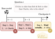
Anecdotal evidence suggests that language models fine-tuned with reinforcement learning exhibit “Aha!” moments—episodes of apparent insight reminiscent of human problem-solving. For example, highlight mid-trace cues such as “Wait… let’s re-evaluate step-by-step,” which sometimes accompany correct answers. Yet, the nature, frequency, and impact of these events (Fig. 1) remain unclear . 1
The existence of “Aha!” moments is linked to whether reasoning models can intrinsically self-correct, i.e., revise their reasoning mid-response without external feedback. Model improvements often arise from extrinsic mechanisms like verifiers, reward queries, prompting techniques, or external tools . In contrast, intrinsic self-improvement must be inferred from reasoning traces and is arguably more safety-relevant, as it implies that a model can reorganize its reasoning from internal state alone .
 />
/>
Studying the effect of reasoning shifts is challenging. First, these events may occur (and affect performance) during training, yet evaluations are typically conducted only post-training . Second, reasoning models rarely release mid-training checkpoints, limiting longitudinal analyses across the training lifecycle. Third, even when shifts are observed, attributing correctness to a mid-trace change (rather than to general competence or memorization) requires systematically controlled comparisons. This gap motivates the need for a systematic investigation of whether reasoning shifts reflect genuine insight.
Present work. Here, we investigate whether mid-trace reasoning shifts (e.g., “Wait… let’s re-evaluate”) signal intrinsic self-correction in reasoning models. Our study is guided by three questions:
RQ1: Do reasoning shifts raise model accuracy?
RQ2: How does the effect of reasoning shifts vary with training stage and decoding temperature?
RQ3: Are reasoning shifts more effective when reasoning models are uncertain?
To answer these, we (i) formalize “Aha!” moments as measurable mid-trace shifts in reasoning that improve performance on problems that were previously unsolved by the model (Fig. 2; §3); (ii) curate a diverse evaluation suite (§4) spanning cryptic crosswords , mathematical problem-solving (MATH-500) , and Rush Hour puzzles ; and (iii) GRPO-tune and annotate the reasoning traces of Qwen2.5 and Llama models (§5).
Our analysis spans $`1`$M+ annotated reasoning traces across hundreds of checkpoint evaluations (10–20 per model/run), 3 domains, 4 temperatures, 2 model sizes, and 2 model architectures, providing a longitudinal view of how mid-trace reasoning evolves during RL fine-tuning. With this setup, we connect shift behavior to both correctness and token-level uncertainty signals .
Our results show that reasoning shifts are rare (overall $`\sim`$6.31% of traces) and generally do not improve model accuracy (RQ1). We further find that their impact on accuracy does not reliably flip sign across training stages, but varies substantially with decoding temperature (RQ2). Finally, we find that spontaneously occurring shifts do not become reliably helpful under high uncertainty; however, externally triggered reconsideration under high entropy improves accuracy across benchmarks, including a +8.41pp improvement on MATH-500 (and smaller gains on crosswords and Rush Hour) (RQ3). Our results are robust across datasets, prompts, and model families.
Contributions. We make three key contributions:
-
Definition & framework. We formalize “Aha!” moments as measurable mid-trace shifts and introduce an experimental framework for studying intrinsic self-correction during RL fine-tuning.
-
Empirical characterization at scale. Across $`1`$M+ traces spanning domains, temperatures, training stages, and model families, we show that reasoning shifts are rare and typically coincide with lower accuracy, challenging the view that they reflect genuine insight.
-
Intervention. We develop an entropy-gated intervention that induces reconsideration when models are uncertain, yielding measurable accuracy gains.
Related Work
Emergent Capabilities. Large language models often appear to acquire new abilities abruptly with scale—such as multi-step reasoning or planning —but it remains debated whether these shifts reflect intrinsic cognitive change or artifacts of evaluation . Many behaviors labeled as “emergent” arise only under extrinsic scaffolds. Structured prompts—e.g., Chain-of-Thought , the zero-shot cue “Let’s think step by step” , or Least-to-Most prompting —elicit intermediate reasoning that models rarely produce on their own. Optimization methods such as SFT , RLHF , and GRPO reinforce these externally induced behaviors, potentially amplifying the appearance of intrinsic ability gains.
Self-Correction and “Aha!” Moments. Self-correction in reasoning models can arise through extrinsic mechanisms—such as verifier models or tool calls —or through intrinsic shifts that occur without any external intervention . Recent work has examined these dynamics, including frameworks for trained self-correction and benchmarks for iterative refinement , and analyses of mid-inference adjustments . Studies of models such as DeepSeek-R1 suggest that reward optimization can induce intrinsic reflection-like artifacts. However, other works have raised doubts about whether observed reasoning shifts reflect genuine insight or superficial self-reflection . Yet, there has been no systematic evaluation of whether RL-trained models exhibit true intrinsic “Aha!”-style self-correction throughout RL fine-tuning, nor whether such shifts reliably improve correctness when tracked across checkpoints and decoding regimes.
Insight Characterization. In cognitive psychology, insight is classically defined as an abrupt restructuring of the problem space, exemplified by ’s chimpanzees stacking boxes to reach bananas. Recent work seeks analogous phenomena in reasoning models: mid-trace uncertainty spikes—sometimes described as “Gestalt re-centering”—have been associated with shifts in reasoning strategy . Metrics such as RASM aim to identify linguistic or uncertainty-based signatures of genuine insight , yet existing approaches misclassify superficial hesitations as insight at high rates in some settings (up to 30%) . These limitations highlight the need for rigorous criteria to distinguish genuine restructurings from superficial reflection.
Safety, Faithfulness, and Alignment. Transparent reasoning traces are central to alignment and faithfulness, as they allow human oversight of not only a model’s outputs but the process that produces them . When self-corrections occur without oversight, they raise concerns about hidden objective shifts or deceptive rationales that can mislead users . Process supervision—rewarding intermediate reasoning steps rather than only final answers—has been shown to improve both performance and interpretability in math reasoning tasks . Complementing this, uncertainty-aware methods help models detect and respond to unreliable reasoning (e.g., via abstention or filtering when uncertainty is high), improving robustness and trustworthiness . Understanding whether mid-trace shifts reflect genuine correction or uncertainty-driven artifacts is therefore directly relevant to evaluating the safety and reliability of reasoning models.
Formalizing “Aha!” Moments
We define an “Aha!” moment as a discrete point within a model’s chain-of-thought where the model abandons its initial reasoning strategy and adopts a qualitatively different one that improves performance. We formalize this notion below.
Let $`\{f_{\theta_k}\}_{k=0}^K`$ denote a sequence of checkpointed
reasoning models. At checkpoint $`k`$, the model defines a policy
$`\pi_{\theta_k}(a_t \mid a_{ denote expected correctness. Let $`S_{q_j,k}(\tau) \in \{0,1\}`$
indicate whether a mid-trace shift occurs in a sampled trajectory
$`\tau`$ at checkpoint $`k`$. This binary label is produced by our
shift-detection pipeline, which identifies lexical and structural
changes in reasoning strategy (detailed in
App. 11.1). We write
$`P(S_{q_j,k}=1)`$ for the probability (under
$`\tau \sim \pi_{\theta_k}`$) that a sampled trace contains a detected
shift. Definition 1 (“Aha!” Moment). Let
$`\delta_1,\delta_2,\delta_3 \in [0,1]`$ be thresholds for prior
failure, prior stability, and required performance gains. An “Aha!”
moment occurs for $`(q_j,k)`$ iff: $`\forall i < k,\; P_{\theta_i}(\checkmark \mid q_j) < \delta_1`$
(Prior failures), $`\forall i < k,\; P(S_{q_j,i}=1) < \delta_2`$ (Prior
stability), $`P_{\theta_k}(\checkmark \mid q_j, S_{q_j,k}=1) - P_{\theta_k}(\checkmark \mid q_j) > \delta_3`$
(Performance gain). In plain terms, a checkpoint $`k`$ qualifies as an “Aha!” moment for
$`q_j`$ if: (1) all earlier checkpoints consistently fail on the problem
(prior failures); (2) earlier checkpoints show little evidence of
mid-trace shifts (prior stability); and (3) at checkpoint $`k`$,
traces containing a detected shift yield a strictly higher correctness
rate than traces overall (performance gain).2 Together, these
conditions ensure that a detected shift is both novel and
beneficial, preventing superficial or noisy variations from being
counted as insight-like events.
Figure 2 illustrates this behavior.
Algorithm [alg:aha-moment] in
App. 11.1 formalizes the detection
procedure. The thresholds $`(\delta_1,\delta_2,\delta_3)`$ act as tunable criteria:
stricter values prioritize precision by requiring consistent prior
failure and rare prior shifts, while looser values increase recall. In
our experiments, we select these thresholds on a held-out development
slab and validate robustness using bootstrap confidence intervals
(App. 12.2). In all
cases, probabilities such as $`P_{\theta_k}(\checkmark \mid q_j)`$ and
$`P_{\theta_k}(\checkmark \mid q_j, S_{q_j,k}=1)`$ are estimated from
finitely many sampled traces per $`(q_j,k)`$. This definition parallels the classical cognitive characterization of
insight: a sudden restructuring of the problem space that enables
solution . Hallmarks of such shifts include explicit self-reflective
cues (e.g., “wait,” “let’s reconsider’’) and an observable pivot in
strategy . Theoretical accounts such as representational change theory ,
progress monitoring theory , and Gestalt perspectives on problem-solving
provide complementary lenses for interpreting analogous shifts in
reasoning models. Our evaluation suite spans three complementary reasoning lenses
(Fig. 3): representational change in
cryptic Xwords (left), quantitative problem solving (center), and
spatial reasoning in RHour–style puzzles (right). Each domain offers
automatic correctness checks, natural opportunities for mid-trace
verification, and structured signals of strategy. All data are in
English; dataset sizes and splits are summarized in
Table 6, and additional filtering and
scoring details are provided in
App. 10.1. Throughout, we score answers
by normalized exact match (canonicalizing case, whitespace, and
punctuation before exact comparison;
App. 10.1). Cryptic Xwords. Cryptic Xwords clues hide a wordplay instruction
(e.g., anagram, abbreviation, homophone) beneath a misleading surface
reading, requiring representational shifts to solve. We train on natural
clues from Cryptonite and evaluate on a
synthetic test set with device-balanced templates
(App. 10.1), scoring by normalized exact
match. Math. Math word problems test symbolic manipulation and multi-step
deduction, with reasoning progress naturally expressed step-by-step. We
train on RHour. We synthetically generate
RHour sliding-block puzzles, where the
goal is to free a target car from a crowded grid by moving obstructing
vehicles. We generate balanced $`4{\times}4`$, $`5{\times}5`$, and
$`6{\times}6`$ boards and evaluate on $`6{\times}6`$ only. Boards are
solved optimally via BFS with per-size node caps, discarding timeouts
(App. 10.1). We filter trivial cases and
stratify remaining instances into easy ($`<`$4 moves), medium
($`<`$6), and hard ($`\geq`$6) buckets by solution
length. We fine-tune reasoning models with GRPO across evaluation domains
(§5.1); collect and annotate reasoning traces
during training (§5.2); and estimate model uncertainty to
trigger entropy-based interventions
(§5.3). Motivated by claims of mid-trace “Aha!” behavior in DeepSeek-R1 , we
adopt Group Relative Policy Optimization (GRPO) as our fine-tuning
method. GRPO is an RLHF-style algorithm that optimizes chain-of-thought
generation by comparing groups of sampled completions and extends PPO
with group-normalized advantages and KL regularization to a frozen
reference policy. Full implementation details appear in
App. 10.4. We fine-tune Qwen2.5 and Llama 3.1 models on each domain for up to
1,000 steps. Our primary experiments use Qwen2.5-1.5B trained for 1,000
steps ($`\approx`$2.5–3 epochs per domain), while larger models
(Qwen2.5-7B and Llama 3.1-8B) are evaluated at 500 steps due to compute
constraints. To verify that models improve during training, we evaluate
at multiple checkpoints and report accuracy at initialization (Step 0)
and at the final evaluated checkpoint (Step 950 for the 1.5B runs;
Step 500 for 7B/8B).
Table 1 summarizes coverage and accuracy
gains. We use lightweight, task-specific prompts that structure reasoning into
a Model coverage and learning progress. Accuracy at initialization
(Step 0) and at the final training checkpoint, along with the absolute
gain ($`\Delta`$). All results are 1-shot evaluations at temperature
$`0`$ on the fixed test sets described in
§4. We evaluate each model at a fixed cadence of every 50 training steps
from initialization (Step 0) to Step 950 inclusive (i.e., checkpoints
$`k\in\{0,50,\ldots,950\}`$), yielding 20 checkpoints per run. At each
checkpoint, we generate $`G{=}8`$ completions per problem using a
fixed decoding policy (temperature $`\{0,0.05,0.3,0.7\}`$,
top-$`p{=}0.95`$). Each completion follows the tag-structured output
contract in
App. 10.2, with private
reasoning in Evaluation sets are held fixed across checkpoints: 500 problems for
MATH-500, 130 synthetic clues for
Xwords, and 500 $`6{\times}6`$ RHour boards. For our Qwen2.5-1.5B
models, because each item is evaluated at all 20 checkpoints across
$`T{=}4`$ temperatures with $`G{=}8`$ samples, each run yields 320,000
Math traces, 83,200 Xwords traces, and 320,000 RHour traces. This
longitudinal structure allows us to track how mid-trace behavior evolves
during RL fine-tuning. We additionally produce 160,000 Qwen2.5-7B traces
and 160,000 Llama3.1-8B traces for
MATH-500 across 10 checkpoints (Step 0 to
Step 450 every 50 steps) to investigate behavior across architecture and
model size. Details about our training and evaluation setup appear in
App. 10.1. To identify reasoning shifts at scale, we use GPT-4o as an LLM-as-judge.
Following evidence that rubric-prompted LLMs approximate human
evaluation , we supply a fixed rubric that scores each trajectory for
(i) correctness, (ii) presence of a mid-trace reasoning shift, and (iii)
whether the shift improved correctness. To reduce known sources of judge bias—position, length, and model
identity effects —we randomize sample order, use split–merge
aggregation, enforce structured JSON outputs, and ensemble across prompt
variants. We also adopt a conservative error-handling policy: we assign
no shift when the cue prefilter fails or when the judge output is
invalid or low-confidence
(App. 11.2). Agreement is high: on
MATH-500, GPT-4o achieves
$`\kappa\!\approx\!0.726`$ across prompt variants and $`\kappa=0.79`$
relative to human majority vote, comparable to expert–expert reliability
. For additional details, see
App. 11.3. For qualitative examples,
see App. 13.6. To relate reasoning shifts to model uncertainty, we measure token-level
entropy throughout each response. At generation step $`t`$, with
next-token distribution $`\mathbf{p}_t`$, we compute Shannon entropy
$`H_t = -\sum_v p_t(v)\log p_t(v)`$. For each completion, we summarize
uncertainty by averaging entropy over the We also study whether uncertainty can be exploited to improve
performance via artificially triggered reflection. In a follow-up
experiment, we test three semantically similar but lexically distinct
reconsideration cues (C1–C3), for example: (C3) “Wait, something is not
right, we need to reconsider. Let’s think this through step by step.”
For each cue, we first obtain the model’s baseline completion (Pass 1),
then re-query the model with the same decoding parameters while
appending the reconsideration cue (Pass 2). We evaluate gains both
overall and under an entropy gate: we split instances into
high-entropy (top 20% within domain) and low-entropy (bottom 80%)
buckets based on Pass 1 sequence entropy, and compare Pass 2 accuracy
across buckets. Cue-specific results and regressions are reported in
App. 12.4. We show that spontaneous reasoning shifts are rare and generally harmful
to accuracy, and that formal “Aha” events are vanishingly rare (RQ1;
§6.1); that this negative effect
remains stable across training stages but varies systematically with
decoding temperature (RQ2;
§6.2); and that extrinsically
triggered shifts reliably improve performance, especially on
high-entropy instances (RQ3;
§6.3). Do reasoning shifts improve accuracy? Before analyzing formal “Aha!”
moments, we first consider the broader class of reasoning shifts—any
mid-trace pivot detected by our annotator, irrespective of whether it
satisfies the stricter criteria in
Def. 1. If such shifts reflected
genuine insight, traces containing them should be more accurate than
those without them. Across domains, temperatures, and checkpoints for Qwen2.5–1.5B,
reasoning shifts remain uncommon (approximately $`7.6\%`$ of samples;
pooling all models/domains yields 6.31%) and are associated with
substantially lower accuracy: $`2.57\%`$ for shifted traces versus
$`16.44\%`$ for non-shifted traces, $`N{=}723{,}200`$. A pooled logistic
regression of correctness on a shift indicator confirms that this
difference is highly significant (p $`< 10^{-1198}`$).3 To test whether this pattern is specific to small GRPO-tuned models, we
evaluate DeepSeekR1 and GPT4o under matched decoding conditions on
MATH. As shown in
Table [tab:external-models], both
models exhibit very low canonical shift rates across temperatures
(0.40–0.60% for DeepSeekR1 and 2.20–3.00% for GPT4o), and accuracy
conditioned on a shift shows no systematic benefit, suggesting that the
phenomenon generalizes across model families and training paradigms.
These results characterize the “raw” behavioral signature of mid-trace
shifts, independent of any stricter “Aha!” interpretation. How frequent are formal “Aha!” moments? We now restrict attention to
the much smaller subset of events that satisfy all three criteria in
Def. 3. In
Fig. 4, by varying
$`\delta_1,\delta_2\in\{0,\,1/8,\,2/8\}`$ and fixing
$`\delta_3=\epsilon>0`$, we find that formal “Aha!” moments are
extremely rare, even with relatively lax constraints. Similar patterns
hold for Qwen2.5–7B and Llama3.1–8B
(App. 12). Pooling every
Crossword/Math/RHour checkpoint and temperature, the formal detector
fires on only $`1.79\%`$ of samples. Robustness checks. As surface cues such as “wait” or “actually”
often fail to track genuine strategy changes , and LLM-judge labels may
pick up prompt- or position-induced biases , we replicate RQ1 using
three detector variants (formal, GPT-based, lexical). All yield the same
conclusion; see
App. 12.6. Takeaway. Reasoning shifts are infrequent and generally harmful to
accuracy. Further, formal “Aha!” moments, which additionally require a
performance gain at the pivot, are vanishingly rare. Neither the general
phenomenon (reasoning shifts) nor its idealized form (“Aha!” moments)
appears to drive problem-solving performance of reasoning models. RQ1 establishes two constraints on “insight-like” behavior: broad
reasoning shifts are uncommon and tend to coincide with worse outcomes,
while formal “Aha!” events are so rare that they contribute little to
overall model performance. This raises a natural question: are we simply
averaging over regimes where shifts sometimes help and sometimes hurt?
We test two plausible sources of heterogeneity: (i) shifts might become
more (or less) effective at different stages of training; and (ii)
their impact might depend on the decoding temperature (and thus
sampling entropy). How does the effect of reasoning shifts vary across training? To
test whether the shift–accuracy relationship changes as training
progresses, we regress correctness on problem fixed effects,
standardized training step, and the shift indicator. We report average
marginal effects (AME) with cluster–robust SEs at the problem level.
4 At $`T{=}0.7`$, we find no evidence that shifts become beneficial later
in training. In Xwords and Math shifts are uncommon
($`\%S{=}2.433`$; $`\%S{=}2.166`$) and are mildly harmful
($`\mathrm{AME}{=}{-}0.0311`$, $`p{=}0.02742`$;
$`\mathrm{AME}{=}{-}0.0615`$, $`p{=}1.55\times10^{-4}`$). In RHour, shifts are comparatively frequent ($`\%S{=}11.449`$) but
have no measurable practical effect on accuracy
($`\mathrm{AME}{\approx}0.0001`$, $`p{\ll}10^{-6}`$). Analogous results
for $`T\in\{0.0,0.05,0.3\}`$ are reported in
Appendix 13.1.
Figure 7a echoes this pattern:
across checkpoints, shifted traces are not systematically more accurate
than non-shifted ones. We repeat robustness checks using alternative
detector variants across $`T\in\{0,0.05,0.3,0.7\}`$ in
App. 13.5. We observe the same qualitative
pattern with the stricter formal “Aha!” detector
(Appendix 13.3), but because it fires
on only $`\approx 10^{-3}`$ of traces at $`T{=}0.7`$, estimates are
underpowered for fine-grained stage-by-stage heterogeneity; critically,
we do not see a consistent late-training transition to positive effects. How does the effect of reasoning shifts vary with decoding
temperature? We next ask whether temperature modulates the
relationship between shifts and correctness. We regress correctness on
problem fixed effects, standardized temperature, and the shift
indicator, aggregating across training steps. 5 Table 3 summarizes the average association between
shifts and correctness while controlling for standardized decoding
temperature (via Raw per-temperature contrasts
(Fig. 6) sharpen the interpretation:
on Xwords, shifts can coincide with productive correction at low
$`T`$, but the benefit weakens and may reverse by $`T{=}0.7`$. In
Math, shifts remain harmful across temperatures, though the raw
penalty attenuates as $`T`$ increases. In RHour, the curve stays close
to zero in magnitude, reflecting the near-zero accuracy regime. Takeaway. We find that reasoning shifts do not reliably yield higher
accuracy across specific training phases or at particular temperatures. The results above (particularly Xwords, see
Fig. 6) suggest that decoding
temperature may modulate the effect of reasoning shifts: at low $`T`$
they sometimes align with productive corrections, while at higher $`T`$
they resemble noise. Because temperature primarily alters sampling
entropy rather than the model’s underlying reasoning process , this
points to a link between shifts and internal uncertainty. We thus ask
whether, under high-uncertainty regimens, reasoning shifts are more
frequent or become more helpful. Are reasoning shifts more likely under high uncertainty? To test
whether shifts preferentially occur when the model is uncertain, we
relate each trace’s reasoning shift indicator to its sequence-level
entropy. We pool traces across all decoding temperatures and training
checkpoints, and fit a logistic regression of shift prevalence on
standardized entropy with problem fixed effects and cluster-robust SEs
(clustered by problem). 6 Pooling all traces across domains (Xwords, Math, RHour), we find
weak evidence that higher entropy is associated with fewer detected
shifts on average (OR$`\approx 0.77\times`$, $`\beta=-0.258`$,
$`\mathrm{SE}=0.143`$, $`p=0.070`$; 95% CI OR $`\in[0.58,1.02]`$;
$`N=723{,}200`$). This aggregate pattern masks domain heterogeneity: the
entropy–shift association is positive in Xwords
(OR$`\approx 2.05\times`$) and RHour (OR$`\approx 1.19\times`$), but
negative in Math (OR$`\approx 0.58\times`$). One possible
interpretation is that in Math, high-entropy generations more often
reflect diffuse exploration or verbose “flailing” rather than a discrete
mid-trace pivot, so the rare, rubric-qualified shifts concentrate in
comparatively lower-entropy traces. Do reasoning shifts improve performance under high uncertainty? A
natural hypothesis is that when the model is uncertain, a mid-trace
pivot might reflect productive self-correction. We test this by
stratifying traces into high-entropy instances (top 20% within domain)
and low-entropy instances (bottom 80%), using a fixed entropy
threshold per domain. Within each stratum, we estimate the effect of a
shift on correctness using a logistic regression with problem fixed
effects and controls for continuous entropy and training step, and
report the shift coefficient alongside the raw accuracy difference
between shifted and non-shifted traces. 7 Table 4 shows that shifts do
not become reliably beneficial in the high-entropy regime. In Math,
shifts remain harmful even among high-entropy traces (raw
$`\Delta=-7.40`$pp) and are substantially more harmful in the
low-entropy majority (raw $`\Delta=-22.88`$pp). In Xwords, the point
estimate in the high-entropy stratum is near zero (raw
$`\Delta=+0.63`$pp), but shifts are rare and estimates are noisy. In
RHour, accuracy is near-zero throughout, so estimated effects are
statistically detectable due to sample size but negligible in magnitude. Can artificially triggered reasoning shifts improve performance? The
negative results above suggest that spontaneous shifts are not a
dependable self-correction mechanism, even when the model is uncertain.
High entropy does not cause more spontaneous pivots; rather, it
identifies instances where a second-pass reconsideration has higher
marginal value. We therefore test an extrinsically triggered “forced
Aha” intervention: for each prompt we generate a baseline completion
(Pass 1), then re-query the model under identical decoding settings
while appending a reconsideration cue (Pass 2), and compare paired
correctness outcomes. Pass 2 uses the same cue across all domains; see
App. 12.4 for the exact
wording and additional analyses. Table 5 reports paired results
aggregated across checkpoints and decoding temperatures. Triggered
reconsideration yields a large gain on Math
($`0.322\!\rightarrow\!0.406`$; $`+8.41`$pp) and a small gain on
Xwords ($`+0.45`$pp), while remaining negligible in absolute terms on
RHour ($`+0.01`$pp) due to its near-zero base rate. The paired “win”
counts show that improvements dominate backslides in Math (50,574
wrong$`\rightarrow`$right vs. 23,500 right$`\rightarrow`$wrong),
indicating that the effect is not merely random flipping. In contrast,
Xwords shows near-balanced wins and losses (5,380 vs. 5,004),
consistent with a much smaller net gain. Finally, consistent with uncertainty serving as a useful gate for
reflection,
Appendix 12.4 shows that these
gains are amplified on high-entropy instances
(Table 18), with a complementary
regression analysis reported in
Table 19. Forced “Aha” (triggered reconsideration), sample-level results. We
compare paired outcomes between a baseline generation (Pass 1) and a
second generation with an appended reconsideration cue (Pass 2).
$`\hat p_{\text{P1}}`$ and $`\hat p_{\text{P2}}`$ denote accuracies in
each pass; $`\Delta`$ (pp) is the percentage-point gain. Takeaway. Reasoning shifts are a low-base-rate event whose
association with entropy varies by domain, and conditioning on
uncertainty does not reveal a “hidden regime” where spontaneous shifts
reliably help. In contrast, artificially triggering reconsideration
yields consistent gains, especially for Math and especially in the
high-entropy tail
(App. 13.7,
Table 18). We formalize and empirically test the notion of intrinsic “Aha!”
moments, mid-trace reasoning shifts that appear to reflect sudden
insight. We find that they are vanishingly rare and that mid-trace
reasoning shifts are typically unhelpful, even in states of high
uncertainty. However, by intervening to trigger reconsideration under
high-entropy conditions, we demonstrate that uncertainty can be
converted into productive reflection, resulting in measurable accuracy
gains. This reframes reasoning shifts not as an emergent cognitive ability, but
as a mechanistic behavior—a byproduct of the model’s inference dynamics
that can nonetheless be harnessed and controlled. Rather than asking
whether models have insight, it may be more useful to ask how and when
they can be made to simulate it. This shift in perspective bridges
recent work on uncertainty-aware decoding , process supervision , and
self-correction , positioning mid-trace reasoning as a manipulable
mechanism for improving reliability rather than genuine insight. Our findings open several directions for further investigation. First,
the link we uncover between uncertainty and the usefulness of
mid-reasoning shifts invites new forms of process-level supervision that
explicitly condition reflection on entropy or confidence estimates .
Second, future work should examine whether RL-based objectives that
reward models for revising earlier answers truly improve reasoning or
merely reinforce uncertainty-responsive heuristics. While recent
approaches such as demonstrate that self-correction can be trained, our
results highlight the need for analyses that disentangle the learning of
reflection-like language from genuine representational changes. It would
be valuable to investigate what the observed dynamics between
uncertainty and mid-reasoning shifts reveal about human insight—whether
uncertainty-driven reconsideration in models mirrors metacognitive
signals in people, or whether the resemblance is purely linguistic.
Bridging computational and cognitive accounts of “Aha!” phenomena could
help identify which internal mechanisms, if any, correspond to genuine
insight. Finally, we hope that this piece inspires more fundamental
research into the impact of RL post-training on model performance: why
do algorithms like GRPO lead to a performance shift if not from improved
reasoning? While our study offers the first systematic analysis of “Aha!” phenomena
in reasoning models, it has several limitations. First, our detection of
reasoning shifts relies on explicit linguistic cues (e.g., “wait,”
“actually”) and measurable plan changes. This makes our estimates
conservative: models may undergo unlexicalized representational changes
that our detector misses, while some detected shifts may instead reflect
superficial hedges. Future work could incorporate hidden-state dynamics
or token-level embeddings to better identify implicit restructurings.
Second, our evaluation spans three reasoning domains but remains limited
to tasks with well-defined correctness signals (math, Xwords, spatial
puzzles). Whether similar patterns hold for open-ended reasoning or
multi-turn interaction remains an open question. Third, our intervention
experiments manipulate model behavior via prompt-level cues rather than
modifying training objectives. Thus, while we demonstrate that
uncertainty-gated reconsideration can improve accuracy, this does not
establish a causal mechanism of internal insight. Extending our analysis
to training-time interventions or process supervision would help clarify
how reflection-like behaviors emerge and generalize. Finally, as with
most large-model studies, our results depend on a small set of families
(Qwen, Llama) and inference hyperparameters (e.g., temperature, sampling
policy). Broader replications across architectures, decoding methods,
larger sizes, and reinforcement-learning setups are necessary to test
the generality of our conclusions. Our study analyzes the internal reasoning behavior of large language
models and does not involve human subjects or personally identifiable
data. All datasets used—MATH-500 ,
Cryptonite , and synthetic
RHour puzzles—are publicly available and
contain no sensitive content. We follow the terms of use for each
dataset and model. Because our work involves interpreting and modifying model reasoning
traces, it carries two potential ethical implications. First, methods
that manipulate mid-trace behavior could be misused to steer reasoning
models toward undesirable or deceptive outputs if deployed
irresponsibly. Our interventions are limited to controlled research
settings and designed to study model uncertainty, not to conceal
reasoning or produce persuasive content. Second, interpretability claims
about “insight’’ or “self-correction’’ risk overstating model
understanding. We therefore emphasize that our findings concern
statistical behavior, not human-like cognition or consciousness. Generative AI tools were used to enhance the search for related works
and to refine the writing and formatting of this manuscript. We followed
the recommendations of , who provide guidance for legitimate uses of AI
in research while safeguarding qualitative sensemaking. Specifically,
Claude, ChatGPT, and Elicit were used to identify relevant research
papers for the Related Work and Discussion sections (alongside
non-generative tools such as Google Scholar and Zotero). After the
Discussion had been written, ChatGPT was used to streamline and refine
the prose, which was then manually edited by the authors. Claude and
ChatGPT were additionally used for formatting tasks, such as generating
table templates and translating supplementary materials to LaTeX. Where
generative AI was used, the authors certify that they have reviewed,
adapted, and corrected all text and stand fully behind the final
content. All model runs, including training and inference, were conducted on
NVIDIA A100 GPUs or NVIDIA A6000 GPUs, with resource management, access
controls, and energy considerations in place. We estimate the total
carbon footprint of all experiments at
approximately 110 kg CO2e, following the methodology of . This work was supported by a First-Year Fellowship from the Princeton
University Graduate School. We are grateful for computational resources
provided by the Beowulf cluster, and we thank the ML Theory Group for
generously sharing additional compute. We also acknowledge the support
of the Center for Information Technology Policy (CITP) and the
Department of Computer Science at Princeton University. We thank our
volunteer annotators and the broader Princeton community. Special thanks
to Cannoli, our lab dog, and to the musical artist, Doechii. This first part of the appendix collects the reproducibility
scaffolding for our experiments: what data we train and evaluate on,
what prompts and output contracts we impose, and how GRPO training is
configured. We begin with dataset sizes and domain-specific
preprocessing details
(§10.1). We then provide the
verbatim system-level prompts used in each domain, including the shared
Table 6 summarizes dataset sizes, splits,
and evaluation coverage for all three reasoning domains. We include
additional details here for reproducibility. We use the Cryptonite corpus for training
and generate synthetic evaluation clues using device-balanced templates.
All answers are normalized (uppercase, punctuation-stripped) before
exact-match scoring. The training distribution is We generate balanced $`4{\times}4`$, $`5{\times}5`$, and $`6{\times}6`$
puzzles and evaluate on $`6{\times}6`$ only. Puzzles are solved
optimally via BFS with per-size node caps; unsolved or degenerate boards
are removed . Solutions are canonicalized before comparison. Code to regenerate the synthetic Cryptic Xwords evaluation set and the
selected RHour puzzles is included in our repository under System Prompt — Cryptic Xwords You are an expert
cryptic-xword solver. Do this (repeat until fully consistent): A) DEVICE
TRIAGE • List plausible devices from anagram, container, reversal,
hidden, charade, deletion, homophone, double def, &lit, letter
selection, substitution, abbr. • For each, quote the indicator
word(s). Reject with a reason. B) PARSE • Mark the **definition** (start
or end). • Mark the **wordplay** with exact fodder + operations. C)
CHECKS • Enumeration must match exactly. • Letter accounting must be
exact (anagram multiset or stepwise build). D) DECIDE • Pick the
candidate best matching definition, indicator(s), and enumeration. • Do
NOT assume anagram without a clear anagrind and fully used fodder. E)
RECONSIDER (if any check fails) • Begin the next <think> with:
"Wait, we need to reconsider. Let’s think this through step by step." •
Say why it failed, then re-run A–D with an alternative device/parse.
FORMAT (no deviations): • Reasoning only in <think>…</think>
• Final entry ONLY (UPPER-CASE) in <answer>…</answer> Clue:
Close, as seen in plaNET EARly (4) <think>Device: HIDDEN;
indicator "as seen in". Def: "Close". Wordplay: hidden in "plaNET EARly"
-> NEAR. Enumeration: (4) OK.</think> <answer> NEAR
</answer> Clue: Mix TEA for a hot drink (3) <think>Device:
ANAGRAM; indicator "Mix". Fodder TEA -> TEA. Def: "a hot drink".
Accounting exact; (3) OK.</think> <answer> TEA
</answer> Clue: Shoe liner at home on fish (6) <think>Device
triage: hidden ? ("on" is not a hidden indicator), anagram ✗ (no
anagrind), charade ✓ ("at home"=IN, "on"=next to), homophone ✗,
... Attempt (HIDDEN) rejected: no indicator; also hidden spans
don’t give (6). Candidate attempt (wrong path): — fails
enumeration/indicator, so we must rethink. Re-evaluate as CHARADES: IN
("at home") + SOLE ("fish") -> INSOLE. Accounting: INSOLE letters: I
N S O L E (6). Definition "Shoe liner" fits. Enumeration (6)
OK.</think> <answer>INSOLE</answer> Our system prompts serve two purposes: (i) scaffold domain-appropriate
reasoning with verifiable intermediate structure, and (ii) standardize
outputs so they are machine-checkable and comparable across checkpoints.
Across all domains we therefore (a) separate private reasoning from the
final response with explicit tags ( System Prompt — Math You are an expert *mathematics
problem-solver. Every time you receive a problem you must: • Analyze it
thoroughly. – Pinpoint the **goal** (what quantity/set/form is
requested). – Pinpoint the **givens/constraints** (domains, integrality,
non-negativity, geometric conditions). – Choose the **methods** to apply
(algebraic manipulation, factorization, inequalities, counting, modular
arithmetic, geometry, calculus, etc.). – Write out the full derivation
that leads to the final result. • Check that the result satisfies all
original constraints (no extraneous roots, correct domain, simplified
form, exact arithmetic). • Respond in **exactly** the tag-based format
shown below – no greeting, no commentary outside the tags. – The final
answer goes inside <answer> **only**. – Use **exact** math
(fractions, radicals, π, e). Avoid unnecessary decimals. – Canonical
forms: integers as plain numbers; reduced fractions a/b with b>0;
simplified radicals; rationalized denominators; sets/tuples with
standard notation; intervals in standard notation. – If there is **no
solution**, write NO SOLUTION. If the problem is **underdetermined**,
write I DON’T KNOW. • You have a hard cap of **750 output tokens**. Be
concise but complete. TAG TEMPLATE (copy this shape for every problem)
<think> YOUR reasoning process goes here: 1. quote the relevant
bits of the problem 2. name the mathematical tool(s) you apply 3. show
each intermediate step until the result is reached If you spot an error
or an unmet constraint, iterate, repeating steps 1–3 as many times as
necessary until you are confident in your result. Finish by verifying
the result satisfies the original conditions exactly
(substitution/checks). </think> <answer> THEANSWER
</answer> We ask models to reason entirely inside Dataset sizes. Training instances are natural clues (Xwords),
problems (Math), and boards (RHour); evaluation uses synthetic clues for
Xwords.
The Xwords prompt encodes established solving practice: device triage
(anagram, container, reversal, hidden, etc.) with quoted indicators,
followed by a two-part parse (definition and wordplay) and two
hard checks: exact enumeration and exact letter accounting. This
combination suppresses common failure modes such as defaulting to
anagrams without a bona fide anagrind or silently dropping letters in
charades. The reconsideration loop is narrow: it requires explaining
why the current attempt fails before proposing an alternative
device/parse. We found this prevents thrashing while still eliciting
genuine mid-trace pivots when a better device is available. Examples in
the prompt illustrate (i) a hidden, (ii) an anagram, and (iii) a
charade—covering the most frequent device classes in our corpus. The math prompt stresses (i) goal/givens/methods triage, (ii) exact,
symbolic manipulation with canonical forms (fractions, radicals,
$`\pi`$, $`e`$), and (iii) end-of-proof validation (domain, extraneous
roots, simplification). We explicitly specify what to output when a
problem is infeasible (“ System Prompt — RHour You are an expert RHour
(N×N) solver. TASK • Input fields are provided
in the user message: - Board (row-major string with ’o’, ’A’, ’B’..’Z’,
optional ’x’) - Board size (e.g., 4x4 or 5x5 or 6x6) - Minimal moves to
solve (ground-truth optimum), shown for training • OUTPUT exactly ONE
optimal solution as a comma-separated list of moves. - Move token =
<PIECE><DIR><STEPS> (e.g., A>2,B<1,Cv3) -
Directions: ’<’ left, ’>’ right, ’^’ up, ’v’ down - No spaces, no
prose, no extra punctuation or lines. GOAL • The right end of ’A’ must
reach the right edge. OPTIMALITY & TIE-BREAKS • Your list must have
the minimal possible number of moves. • If multiple optimal sequences
exist, return the lexicographically smallest comma-separated sequence
(ASCII order) after normalizing tokens. VALIDATION • Tokens must match:
^[A-Z][<>^v]+̣(,[A-Z][<>^v]+̣)*$ • Each move respects vehicle
axes and avoids overlaps with walls/pieces. • Applying the full sequence
reaches the goal with exactly moves moves. IF INCORRECT /
UNVALIDATED • Repeat reasoning process, iterating until correct. FORMAT
• Answer in the following way: <think> Your reasoning
</think> <answer> A>2,B<1,Cv3 </answer> For RHour puzzles, the prompt formalizes the interface between
natural-language reasoning and a discrete planner. Inputs are normalized
($`N\times N`$ board, row-major encoding), and The full configs, exactly as used for training, are available in our
repository under To probe how sensitive performance is to system-prompt wording, we
evaluated $`K{=}5`$ paraphrased system prompts for Prompts are released verbatim below. We use the same decoding policy
across checkpoints (temperature, top-$`p`$, stop criteria), cache RNG
seeds, and reject outputs that violate the format contracts before
computing task-specific rewards. This protocol ensures that improvements
in correctness or in “Aha!” prevalence reflect changes in the model’s
internal state rather than changes in instructions or graders. Figures
8,
9,
10 show our verbatim system level
prompts. We fine-tune instruction models (Qwen 2.5–1.5B, Qwen 2.5–7B,
Llama 3.1–8B) with Group Relative Policy Optimization (GRPO) , using
task-specific, tag-constrained prompts that place private reasoning in
We use the OpenR1 GRPO trainer with a vLLM inference server for
on-policy rollouts and All rewards are per-sample and clipped to $`[0,1]`$. Xwords. Exact match on the inner Math. Requires the full tag template; the gold and predicted
RHour. Composite score combining exact (canonical token
sequence), prefix (longest common prefix vs. gold), solve (shorter
optimal solutions $`\uparrow`$), and a planning heuristic $`\Phi`$
(distance/blockers decrease $`\uparrow`$); when a board is provided we
legality-check and simulate moves, otherwise a gold-only variant
supplies solve/prefix shaping. Defaults (used here):
$`w_\text{exact}{=}0.65`$, $`w_\text{solve}{=}0.20`$,
$`w_\text{prefix}{=}0.10`$, $`w_\Phi{=}0.05`$. Across runs we use cosine LR schedules with warmup, clipped
advantages/values, and KL control targeting
$`\text{KL}_\text{target}\!\approx\!0.07`$ via an adaptive coefficient
($`\beta`$) with horizon $`50`$k and step size $`0.15`$; value loss
weight $`0.25`$; PPO/GRPO clip ranges $`0.05`$–$`0.10`$ depending on
run; horizon $`1024`$; $`\gamma{=}0.99`$, $`\lambda_\text{GAE}{=}0.95`$. We use fixed system prompts per domain that enforce exact formatting (no
deviation), encourage compact reasoning, and cap Table [tab:grpo-configs] summarizes only
the run-level choices that differ by domain/model; all other defaults
follow the overview above. We train with ZeRO-3 (stage 3), CPU offload for parameters and
optimizer, and the standard single-node launcher; the provided
Jobs were launched under Slurm on 8-GPU nodes, using a mix of NVIDIA
A100 and RTX A6000 GPUs. For the Qwen2.5-1.5B runs, we reserve
one GPU for vLLM rollouts and use the remaining GPUs for
This appendix details the pipeline used to (i) label mid-trace reasoning
shifts in individual generations and (ii) operationalize formal “Aha!”
events as a checkpoint-level phenomenon. We first present our formal
“Aha!” detector, which combines prior-failure, prior-stability, and
conditional-gain criteria
(App. §11.1). We then describe the
trace-level shift annotation protocol used throughout the paper
(App. §11.2). Finally, we document the
LLM-as-a-judge reliability protocol and the human-labeling template used
for validation
(App. §11.3 and
App. §11.4). Alg. [alg:aha-moment] operationalizes
Def. 1 and
Fig. 2 via three checks: Prior failures: for $`q_j`$, all checkpoints $`i Prior stability: mid-trace shifts are rare for $`i Conditional gain at $`k`$: when a mid-trace shift occurs at
$`k`$, expected correctness increases by a prescribed margin. For each pair $`(q_j,k)`$ we draw $`M`$ independent traces
$`\tau^{(m)} \sim \pi_{\theta_k}(\cdot \mid q_j)`$ under a fixed
decoding policy (temperature $`\tau`$, top-$`p`$, and stop conditions
held constant across $`k`$): For the conditional estimate we average only shifted traces at $`k`$: with a tiny $`\epsilon`$ (e.g., $`10^{-6}`$) to avoid division by zero.
If the denominator is $`0`$, Step 3 is inconclusive and the procedure
returns . We mark a generation as shifted if it contains both: (i) a lexical
cue of reconsideration (e.g., “wait”, “recheck”, “let’s try”, “this
fails because …”), and (ii) a material revision of the preceding plan
(rejects/corrects an earlier hypothesis, switches method or candidate,
or resolves a contradiction). We implement this with a conservative
two-stage detector (lexical cue prefilter + rubric-guided adjudication)
described in
App. §11.2. To calibrate superficial
hedges and edge cases, we tuned thresholds for the cue matcher and
clamping on a small, human-verified set
(App. §11.4). For each $`i and we require $`\widehat{\Pr}[S_{q_j,i}{=}1] < \delta_2`$ for all
$`i We set $`(\delta_1,\delta_2,\delta_3)`$ on a held-out development slab
by maximizing F1 for Aha
vs. non-Aha against human labels. Unless
stated otherwise, we use $`\delta_1{=}0.125`$ (prior correctness
ceiling), $`\delta_2{=}0.125`$ (shift-rate ceiling), and
$`\delta_3{=}0.125`$ (minimum gain). To guard against Monte Carlo noise
in $`\hat P`$, we further require the one-sided bootstrap CI (2000
resamples over traces) for
$`\hat P_{\theta_k}(\checkmark \mid q_j, S{=}1) - \hat P_{\theta_k}(\checkmark \mid q_j)`$
to exceed $`0`$ at level $`\alpha{=}0.05`$. If this test fails, Step 3
returns . Step 1: Prior failures Step 2: Prior stability Step 3: Performance gain
$`p_k \gets P_{\theta_k}(\text{correct}\mid q_j)`$
$`p^{\text{shift}}_{k} \gets P_{\theta_k}(\text{correct}\mid q_j,\; S_{q_j,k}{=}1)`$ Unless noted otherwise, we use $`M{=}8`$ samples per $`(q_j,k)`$,
top-$`p{=}0.95`$, temperature $`\tau{=}0.7`$, and truncate at the first
full solution (math), full entry parse (xword), or solved board state
(RHour). We cache RNG seeds so cross-checkpoint comparisons differ only
by $`\theta_k`$. The detector uses $`O(JKM)`$ forward passes (plus inexpensive
prefiltering and adjudication), where $`J`$ is the number of items and
$`K`$ the number of checkpoints. We cache
$`\{\tau^{(m)}, R(\tau^{(m)}), S(\tau^{(m)})\}`$ per $`(q_j,k)`$ for
reuse in ablations (temperature sweeps, entropy bins). (i) If any $`i For each $`(q_j,k)`$ we log: the prior-failure margin
$`\delta_1-\max_{i Our shift detector may miss unlexicalized representational changes
(false negatives) and can be triggered by surface hedges if the
adjudicator fails (false positives). The bootstrap addresses variance
within checkpoints but not dataset shift across checkpoints; we
therefore hold decoding hyperparameters fixed across $`k`$. We flag a binary shift in reasoning inside the Extract $`t \leftarrow \tau.\texttt{ Given checkpointed JSONL outputs, we annotate each trace in four steps: Parse. Extract Cue prefilter (A). Search Material revision check (B). For prefilter hits, query an LLM
judge (GPT–4o) with a rubric that restates (A)+(B) and requests a
strict JSON verdict plus short before/after excerpts around the
first cue. If the verdict is uncertain or invalid, assign FALSE. Record. Write the Boolean label and minimal diagnostics
(markers, first-cue offset, excerpts) back to the record; processing
order is randomized with a fixed seed. The procedure is
idempotent—existing labels are left unchanged. This conservative policy (requiring both an explicit cue and a
substantiated revision, and defaulting to FALSE on uncertainty)
keeps false positives low and yields conservative prevalence estimates. LLM-as-a-Judge — System Prompt (Shift in Reasoning) You
are a careful annotator of single-pass reasoning transcripts. Your task
is to judge whether the writer makes a CLEAR, EXPLICIT "shift in
reasoning" within <think>...</think>. A TRUE label requires BOTH: (A) an explicit cue (e.g., "wait", "hold
on", "scratch that", "contradiction"), AND (B) a material revision of
the earlier idea (reject/correct an initial hypothesis, pick a new
candidate, fix a contradiction, or change device/method). Do NOT mark TRUE for rhetorical transitions, hedging, or generic
connectives without an actual correction. Judge ONLY the content inside
<think>. Be conservative; these events are rare. LLM-as-a-Judge — User Template (filled per example)
Problem/Clue (if available): problem PASS-1 <think> (truncated if long): think Heuristic cue candidates (may be empty): cues
first_marker_pos: pos Return ONLY a compact JSON object with keys: - shift_in_reasoning:
true|false - confidence: "low"|"medium"|"high" - markers_found: string[]
(verbatim lexical cues you relied on) - first_marker_index: integer
(character offset into <think>, -1 if absent) - before_excerpt:
string (<=120 chars ending right before the first marker) -
after_excerpt: string (<=140 chars starting at the first marker) -
explanation_short: string (<=140 chars justification) To bias the LLM-as-a-judge toward explicit reconsideration, we
pre-filter traces using a hand-crafted list of lexical cues. Concretely,
we match case-insensitive regex patterns over the @ l Y @ Category & Representative cues (lemmas/phrases) We reject as insufficient evidence: (i) bare discourse markers without
correction (but, however, therefore, also); (ii) hedges or
meta-verbosity (maybe, perhaps, I think, let’s be careful)
without an explicit pivot; (iii) formatting or notational fixes only;
(iv) device/method names listed without rejecting a prior attempt; and
(v) cues appearing outside The judge must justify that the post-cue span negates or corrects a
prior claim, selects a different candidate, changes the solving
device/method, or resolves a contradiction. We store short
If the judge call fails or returns invalid JSON, we save the prompt to a
local log file, stamp FALSE, and continue. We clamp long We fix a shuffle seed for candidate order, sort files by natural
The whitelist privileges explicit cues and may miss unlexicalized
pivots (false negatives). Conversely, some cues can appear in
non-revisional discourse; the material-revision test mitigates but does
not eliminate such false positives. Because we default to FALSE on
uncertainty, prevalence estimates are conservative. We use GPT–4o as a scalable surrogate for shift annotation and address
known judge biases—position, length, and model-identity—with a
three-part protocol : Order randomization. We randomly permute items and (when
applicable) apply split–merge aggregation to neutralize position
effects . Rubric-anchored scoring. GPT–4o completes a structured JSON
rubric, following G-Eval-style guidance . Prompt-variant stability. We re-query with $`K{=}5`$
judge-prompt variants at judge temperature $`0`$ and report
inter-prompt agreement. Table 7 lists the five judge prompt variants;
Table [tab:judge-reliability-ckpt]
summarizes inter-prompt agreement on a fixed evaluation set. Judge prompt variants v1–v5 used for shift-in-reasoning annotation. For each trajectory we record: (i) graded correctness, (ii)
shift/no-shift label, (iii) whether a shift improved correctness, (iv)
GPT–4o’s confidence (low/med/high), and (v) auxiliary statistics (e.g.,
entropy). This separation supports analyses of shift prevalence versus
shift efficacy. Before judging, we apply a cue-based prefilter
(App. §11.2). Empirically, responses
without cue words almost never contain qualifying shifts (human
annotation of 100 such responses from Qwen-1.5B on
MATH-500 found none). We evaluated Qwen-1.5B (GRPO) on
MATH-500, using five paraphrased judge
prompts (v1–v5), randomized item order, and judge temperature $`0`$.
Table [tab:judge-reliability-ckpt]
reports percent agreement (PO), mean pairwise Cohen’s $`\kappa`$, and
95% bootstrap CIs. Relative to a human majority-vote reference on 20 examples, GPT–4o
achieved Cohen’s $`\kappa=0.794`$ with PO$`=0.900`$. Mean human–human
agreement was lower (PO$`=0.703`$, mean pairwise $`\kappa=0.42`$), and
mean LLM–human agreement was intermediate (PO$`=0.758`$, mean pairwise
$`\kappa=0.51`$).
Table 8 summarizes these
comparisons. Human validation of shift labels. We compare GPT–4o shift judgments
against a human majority-vote reference on a 20-item validation set (PO
= percent agreement). We also report mean pairwise Cohen’s $`\kappa`$
among human annotators and between GPT–4o and individual humans on the
same items. We include the full rubric and sample items from our human annotation
survey in
App. §11.4. We used $`6`$ volunteer adult annotators (unpaid), recruited from the
authors’ academic networks. Participants gave informed consent on the
task page and could withdraw at any time. No sensitive personal
information was requested. This activity consisted solely of judgments about model-generated text
and did not involve collection of sensitive data or interventions with
human participants. Under our institutional guidelines, it does not
constitute human-subjects research; consequently, no IRB review was
sought. Items were shown in randomized order. Annotators saw the original
Question asked and the verbatim Primary label: Yes/No (shift present). Optional fields: confidence
(low/med/high), first cue index (character offset), and a one-sentence
rationale. Edge cases defaulted to No unless a method switch (e.g.,
completing-the-square $`\to`$ factoring; permutations $`\to`$
stars-and-bars; prime factorization $`\to`$ Euclidean algorithm) was
evident. Annotators completed a short calibration set (including Examples A–H)
with immediate feedback. During labeling we interleaved hidden gold
items and monitored time-on-item; submissions failing pre-registered
thresholds were flagged for review. Each item received independent labels. We report Cohen’s $`\kappa`$ with
95% bootstrap CIs. We did not collect sensitive demographics. Released artifacts include
prompts, anonymized traces (with Read the model’s (1) The model clearly switches strategies mid-trace. (2) It abandons
one method after noticing a contradiction, dead end, or mistake, and
adopts a different method. (3) This is a real strategy pivot, not a
small fix. (1) The model keeps using the same method throughout. (2) It only
makes minor arithmetic/algebra fixes. (3) It adds detail or notation
without changing approach. Important: cue words alone (“wait”,
“recheck”, etc.) do not count; look for an actual method switch. Identify the initial method. Look for a pivot: does the model drop
that plan and adopt a different method? Ignore small fixes. Answer
Yes only with a clear pivot; otherwise No. Question. How many sides would there be in a convex polygon if the sum
of all but one of its interior angles is $`1070^\circ`$? Model Correct answer: Yes. Why: Notices a contradiction and switches
approach. Question. Simplify $`3/\sqrt{27}`$. Model Correct answer: No. Why: One method throughout (simplify radical
$`\to`$ rationalize). Question. Solve $`x^{2}-5x-14=0`$. Model Correct answer: Yes. Why: Switch from completing the square to
factoring. Question. Compute
$`\dfrac{d}{dx}\left(\dfrac{x^{2}+3x+2}{x+1}\right)`$. Model Correct answer: No. Why: Stays with quotient rule; no pivot. Question. How many nonnegative integer solutions $`(x,y)`$ satisfy
$`x+y=20`$? Model Correct answer: Yes. Why: Pivot from permutations framing to
stars-and-bars. Question. What is the sum of the first $`50`$ odd integers? Model Correct answer: No. Why: Single recalled formula; no change in
method. Question. Find $`\gcd(252,198)`$. Model Correct answer: Yes. Why: Abandons prime factorization for
Euclidean algorithm. Question. Solve the system $`x+y=10,\; xy=21`$. Model Correct answer: No. Why: One consistent quadratic/Vieta
approach. Annotation Questions, Verbatim. Then, our annotators are asked to
provide Yes/No answers as to whether a shift in reasoning occurred for
the following $`20`$ questions. We have included one sample question
here, to provide an example of the task: Question Asked: If $`a`$ and $`b`$ are positive integers such that
$`\gcd(a,b)=210`$, $`\mathop{\text{lcm}}[a,b]=210^3`$, and $`a Model Response: <think>The greatest common divisor (GCD) of $`a`$
and $`b`$ is given as $`210`$, and their least common multiple (LCM) is
$`210^3`$. This implies that both $`a`$ and $`b`$ share the prime
factors of $`210`$, which are $`2`$, $`3`$, and $`5`$. Let’s express $`a`$ and $`b`$ in terms of their prime factorizations: Given that $`\gcd(a,b) = 210 = 2^1 \cdot 3^1 \cdot 5^1`$, we get the
following equations from comparing exponents: For the GCD: For the LCM: Thus, Since $`\mathop{\text{lcm}}[a,b] = 210^3`$, substituting the values
gives us: This simplifies our expressions for $`w`$, $`v`$, and $`t`$ to: Therefore, the only combination satisfying these conditions is: Substituting back into the expression for $`a`$ yields: However, since $`a < b`$, this alone does not provide any new
information because $`a = b`$. To find all pairs $`(a, b)`$ where $`a < b`$ and $`\gcd(a, b) = 210`$: -
We need to consider all combinations of $`a`$ and $`b`$ such that: Considering $`x > x'`$, $`y > y'`$, and $`z > z'`$: - For $`x > x'`$: Since $`x`$ cannot be greater than 1 (as $`a`$ must
be less than $`b`$), the only possibility is $`x' = 0`$ (i.e., $`a`$ can
take on any power of 2 except 0, making $`a = 210k`$ where $`k`$ is some
integer). - Similarly, considering $`y > y'`$ and $`z > z'`$, the same logic
applies for powers of 3 and 5 respectively. Thus, $`a`$ could be $`210 \cdot 3^m \cdot 5^n`$ for various
combinations of $`m`$ and $`n`$. Each choice of $`m`$ and $`n`$ uniquely determines $`a`$, resulting in
infinitely many possible values of $`a`$ because there are infinitely
many integers $`m`$ and $`n`$.</think> Fill-in-the-bubble response. Choices: Yes / No (no alternative /
third choice was provided). LLM-as-a-Judge assessed answer. “Yes”. Post-assessment, we reveal the LLM-as-a-Judge answer to participants and
encourage them to invite others to participate. Each individual’s score
was weighted equally, and we analyzed annotator agreement as described
in 11.3. The complete assessment
is made available as part of our codebase. This appendix collects supplementary analyses that extend and
stress-test the main results. We first report the prevalence of formal
“Aha!” events under threshold grids and summarize cross-domain patterns
(App. §12.1). We then
replicate key regressions and uncertainty analyses on larger model
families (Qwen2.5–7B and Llama 3.1–8B) to verify that the shift effects
generalize beyond Qwen2.5–1.5B
(App. §12.3). Next, we test whether
entropy-gated, extrinsically triggered reconsideration is robust to
the specific cue wording
(App. §12.4). Finally, we
evaluate external models (DeepSeekR1 and GPT4o) under the same
shift-detection protocol and compare alternative shift detectors
(App. §12.5 and
App. §12.6). Together, these
checks show that our qualitative conclusions are stable across domains,
model families/sizes, prompt variants, and detector choices. Each panel reports the share of problem–checkpoint pairs $`(q_j,k)`$
that satisfy our operational definition of an “Aha!” moment
(Def. 1) under a grid of thresholds:
$`\delta_1\!\in\!\{0,\tfrac{1}{8},\tfrac{2}{8}\}`$ (maximum prior
accuracy), $`\delta_2\!\in\!\{0,\tfrac{1}{8},\tfrac{2}{8}\}`$ (maximum
prior shift rate), and, unless noted, $`\delta_3=\epsilon>0`$ (any
non-zero gain at $`k`$). Cells show the percentage and the raw counts
$`(\#\text{events}/\#\text{pairs})`$. We aggregate over checkpoints
$`\leq\!1000`$ with $`G{=}8`$ samples per item, and we use the
conservative detector described in
App. 11.2 (lexical cue and material
revision; default to FALSE on uncertainty). Three robust trends emerge across Xword, Math, and RHour and
across model families/sizes. Rarity. Even under the lenient gain criterion
$`\delta_3\!=\!\epsilon`$, “Aha!” events occupy a very small fraction
of problem–checkpoint pairs. Most cells are near zero; none approach a
large fraction. This mirrors the main-text finding that mid-trace
shifts seldom coincide with measurable improvements. Sensitivity to prior instability and prior accuracy. Relaxing
either prerequisite increases counts but remains small in magnitude.
In particular, moving to higher $`\delta_2`$ (allowing more prior
shifts, i.e., lower prior stability) and higher $`\delta_1`$ (allowing
occasional prior solves) produces the visually “warmest’’
cells—consistent with the intuition that “Aha!” detections concentrate
where traces have shown some volatility and the item is not maximally
hard. Domain/model differences. RHour exhibits a higher raw shift
rate (App. §6.2), but the “Aha!” filter
(requiring a gain at $`k`$) prunes most cases; the absolute prevalence
remains low. Xword shows small pockets of higher prevalence when
$`\delta_1,\delta_2\!\geq\!\tfrac{1}{8}`$, whereas Math is uniformly
sparse. Scaling from Qwen 1.5B to 7B or switching to Llama 3.1–8B does
not materially increase prevalence. Replacing $`\delta_3{=}\epsilon`$ with a minimal absolute lift (e.g., at
least one of the $`G{=}8`$ samples flips from incorrect to correct at
$`k`$) further reduces counts but preserves the qualitative ordering
across domains and models. Across all settings, formal “Aha!” moments—requiring both a mid-trace
reasoning pivot and a contemporaneous performance gain—are vanishingly
uncommon. The sparse, threshold-stable patterns in
Figs. 16–17 show this
finding across temperatures, domains, and models. To make our threshold-selection procedure concrete, we ran the
grid/bootstrapped threshold search across the stored Qwen2.5–1.5B
evaluation outputs for each domain and temperature. For each domain$`\times`$temperature root, we searched a small grid
$`\delta_1,\delta_2\in\{0,1/8,2/8\}`$ and
$`\delta_3\in\{\text{None},0,0.05,0.125\}`$ (with Across these stored outputs, the selected thresholds yield extremely low
event prevalence, and gains are generally small, unstable, or negative.
In particular, for Math at $`T\in\{0.05,0.3\}`$ the best available
configurations (under this search) have negative bootstrap lower
bounds, indicating no robust evidence that shifted traces outperform the
baseline on the flagged pairs. We extend the main-text analysis to probe the role of model family and
size. Replicating the raw-effect analyses for Qwen2.5–7B and
Llama 3.1–8B on Math, we observe the
same qualitative pattern reported for Qwen2.5–1.5B: mid-trace
reasoning shifts are consistently detrimental across training steps and
remain negative across decoding temperatures (magnitudes vary, not the
sign), matching
Fig. 15 and
Table 9. We begin by checking whether the core RQ1 finding about rarity
generalizes across model family and size. Using the same formal detector
(Def. 1) and threshold grid as in the
main text, we compute the fraction of problem–checkpoint pairs that
qualify as “Aha!” events.
Fig. 12 shows that these
events remain extremely sparse for both Qwen2.5–7B and Llama 3.1–8B
(Math, $`T{=}0.7`$). We then repeat the regression analysis from
Table 3 for these models.
Figure 15 visualizes the raw
effect across training steps and decoding temperatures. This appendix extends the main-text uncertainty analysis to larger model
families on Math, using traces from
Qwen2.5–7B and Llama 3.1–8B. Our goal is to test a simple
hypothesis: if reasoning shifts are primarily an uncertainty response,
then shifts should become more likely as uncertainty rises. We
operationalize uncertainty using each trace’s sequence-level entropy
and use the same GPT-derived binary shift indicator as in the main text. For each decoding temperature $`T`$, we regress the shift indicator on
standardized sequence entropy with problem fixed effects and
cluster-robust standard errors clustered by problem: Across both model families, we again find a non-positive association
between entropy and shift prevalence. In particular, at $`T{=}0.05`$ and
$`T{=}0.7`$, a 1 SD increase in entropy significantly reduces the odds
of a detected shift (OR$`_{1\sigma}{=}0.63`$, $`p{=}0.001294`$;
OR$`_{1\sigma}{=}0.67`$, $`p{=}0.002396`$), while the estimates at
$`T{=}0`$ and $`T{=}0.3`$ are not distinguishable from zero. This
mirrors the smaller Qwen2.5–1.5B Math
models: shifts are not more common in high-entropy regimes, and when a
dependence is detectable, it points in the opposite direction. To complement the prevalence analysis,
Table 10 stratifies the
raw shift effect on correctness by entropy (high = top 20%, low =
bottom 80%), pooling temperatures and restricting to early training
steps (steps $`\le\!450`$). The qualitative picture is consistent across
strata: shifts are associated with lower accuracy even within the
high-entropy slice. Finally,
Table 11 reports paired
sample-level results for triggered reconsideration (Pass 2). This
manipulation differs from spontaneous shifts: it explicitly prompts the
model to re-evaluate. On Math, forced
reconsideration yields a positive gain for Qwen2.5–7B ($`+5.97`$pp)
but a negative gain for Llama 3.1–8B ($`-4.19`$pp) in this
evaluation slice. We tested only on a subset given the high compute
cost. Forced “Aha” (triggered reconsideration), sample-level results on
Math. $`\hat p_{\text{P1}}`$ and
$`\hat p_{\text{P2}}`$ are accuracies in baseline vs. forced pass;
$`\Delta`$ is the percentage-point gain; “wins” count paired samples
where one pass is correct and the other is not. To test whether the effect of artificially triggered reflection depends
on the specific reconsideration cue used, we evaluate three semantically
similar but lexically distinct prompts: C1: “Hold on, this reasoning might be wrong. Let’s go back and
check each step carefully.” C2: “Actually, this approach doesn’t look correct. Let’s restart
and work through the solution more systematically.” C3: “Wait, something is not right; we need to reconsider. Let’s
think this through step by step.” For each cue, we re-run $`8\times 500`$ Math problems (Qwen2.5–1.5B,
final checkpoint) with 1-shot decoding at $`T{=}0.1`$, obtaining $`500`$
paired baseline and cued completions per cue. We then fit a logistic
regression for each cue, controlling for baseline correctness and
problem identity.8 Across all cues, higher entropy is strongly associated with improved
post-intervention accuracy.
Table 12 reports standardized entropy
coefficients, unit odds ratios (raw entropy), and odds ratios for a 1 SD
increase in entropy. Entropy-gated improvement under three reconsideration cues.
$`\beta`$ is the coefficient on standardized entropy from a logistic
regression controlling for baseline correctness and problem fixed
effects; brackets give 95% CIs. OR is the unit odds ratio (raw entropy),
and OR$`_{1\sigma}`$ is the odds ratio for a $`1`$ SD increase in
entropy. All three cues show the same qualitative pattern: a one–standard
deviation increase in entropy substantially increases the odds of
correctness after the reconsideration cue (2.2$`\times`$–2.5$`\times`$
across cues). C2 yields the strongest effect, but the differences are
modest, indicating that the intervention’s success is tied to
uncertainty rather than to any particular lexical phrasing. To verify that our findings are not an artifact of the GRPO-tuned models
studied in the main paper, we evaluate two widely discussed reasoning
models—DeepSeekR1 and GPT4o—under our shift-detection protocol. These
models have been cited as exhibiting frequent “Aha!” moments or dramatic
mid-trace realizations , making them a natural stress test for our
methodology. We evaluate both models on the full MATH
benchmark with: 1-shot decoding, temperatures $`T\in\{0, 0.05\}`$, identical prompting format (with no system-level alterations or heuristics. Each model generates exactly one chain-of-thought sample per problem,
yielding $`N{=}500`$ traces per model per temperature. We use the same annotation protocol as in
§5.2 and
App. 11.2: Cue prefilter: at least one explicit lexical cue of
reconsideration (e.g., “wait”, “actually”, “hold on”), using the
whitelist in
Table [tab:shift-cue-whitelist]. Material revision: GPT4o judges whether the post-cue reasoning
constitutes a genuine plan pivot (rejecting a candidate, switching
method, resolving a contradiction), returning a strict JSON verdict. Cases lacking either (A) lexical cue or (B) structural revision are
labeled as no shift. Table [tab:external-models] shows
shift prevalence and conditional accuracy by decoding temperature. Both
models exhibit low canonical shift base rates under our definition.
For GPT4o, conditional accuracy given a shift is not reliably higher
than the non-shift baseline: at $`T{=}0.05`$, shifted traces are
substantially less accurate ($`P(\checkmark\mid S{=}1)=0.18`$
vs. $`P(\checkmark\mid S{=}0)=0.724`$), and at $`T{=}0`$ shifted traces
are also lower ($`0.60`$ vs. $`0.724`$). For DeepSeekR1, the number of
shifted traces is extremely small (2–3 traces), so conditional
comparisons are unstable. These results reinforce two conclusions: Low base rate of canonical shifts. Even high-capability
reasoning models produce criteria-satisfying mid-trace pivots only
rarely. Canonical shifts do not reliably improve accuracy. Conditional
accuracy given a shift is unstable across temperatures and does not
show a consistent benefit. We release the full set of model outputs and shift annotations used in
this analysis on Hugging Face; see
Table 13. Released external-model outputs. Hugging Face datasets containing
1-shot MATH-500 traces used in
App. §12.5, for $`T\in\{0,0.05\}`$. Prior work shows that superficial linguistic markers of hesitation—such
as “wait,” “hold on,” or “actually”—are unreliable indicators of genuine
cognitive shifts. Keyword-based detectors misclassify such cues at high
rates, often interpreting hedges or verbosity as insight-like events .
Recent analyses of “Aha!”-style behavior in LLMs similarly report that
many mid-trace cues reflect shallow self-correction or filler language
rather than substantive plan changes . In parallel, LLM-as-a-judge evaluations are known to exhibit position,
ordering, and verbosity biases unless structured and controlled .
Because our primary shift detector uses an LLM-as-judge, it is important
to verify that conclusions do not depend on the specific annotation
mechanism. We replicate the full RQ1 analysis using three detectors: (i) a strict
formal “Aha!” criterion
(Def. 1), (ii) our rubric-guided
GPT-based shift detector used in the main text, and (iii) a permissive
lexical-only detector that flags any cue-phrase occurrence.
Table [tab:alt-shift-detectors]
summarizes results for Qwen2.5–1.5B at $`T=0.7`$. Formal Aha ( GPT-based shifts ( Lexical-only shifts ( For each detector, domain, and item we compute: (i) shift prevalence
$`\%S`$, (ii) accuracies $`\hat p_{Y\mid S=1}`$ and
$`\hat p_{Y\mid S=0}`$, (iii) the raw accuracy difference
$`\Delta\% = 100\cdot(\hat p_{Y\mid S=1}-\hat p_{Y\mid S=0})`$
(percentage points), and (iv) the average marginal effect (AME) of a
shift from a logistic regression with problem fixed effects and
cluster-robust SEs (shown with $`p`$-value). Two patterns are consistent across domains: Shifts are rare under every detector. Even the most permissive
lexical detector ( Shifts are non-beneficial to accuracy. Raw differences
$`\Delta\%`$ and AMEs are non-positive across domains and detectors,
with the only exception being Math
under the strict Overall, this robustness check confirms that our main RQ1 conclusion
does not depend on the specific shift detector: whether we use the
strict formal This appendix collects supplementary tables and figures that expand the
main-text analyses and document additional aggregations that are
referenced in our scripts but not surfaced elsewhere in the paper. We
provide: (i) training-stage regressions at fixed decoding temperatures
(beyond the $`T{=}0.7`$ slice in the main text), (ii) temperature sweeps
for the stricter formal “Aha!” detector, (iii) analogous
temperature/stage breakdowns for larger models (Qwen2.5–7B and
Llama 3.1–8B) on Math, and (iv)
additional uncertainty-gated intervention summaries, including pooled
Qwen-1.5B and 7B/8B entropy-regression results. All tables use the same
conventions as the main text: $`\%S`$ is shift prevalence,
$`\Delta\mathrm{pp}`$ denotes a raw accuracy difference in percentage
points, and AMEs/coefficients come from Binomial(logit) models with
problem fixed effects and cluster-robust SEs (clustered by problem). Table 14 replicates the
training-stage analysis from
Table 3, holding the decoding temperature fixed at
$`T\in\{0.0,0.05,0.3\}`$. Across these settings, we again find no
evidence that reasoning shifts become beneficial later in training. In
Math, shifts are consistently harmful across all temperatures. In
RHour, accuracies are near zero for both shifted and non-shifted
traces, and the estimated effects are practically negligible. Table 15 provides the same
fixed-temperature, training-stage analysis as
Table 14, but for larger models on
Math (Qwen2.5–7B and Llama 3.1–8B),
evaluated over steps $`\le 450`$. Across temperatures, shifts remain
associated with lower accuracy; the magnitude of the raw penalty varies
with $`T`$ and model family, but does not reverse sign. We repeat the temperature-sweep analysis using the stricter formal
“Aha!” detector (Def. 3.1), which requires a mid-trace pivot and a
contemporaneous performance gain at that checkpoint. For each decoding
temperature $`T\in\{0,0.05,0.3,0.7\}`$, we estimate the association
between correctness and the formal-Aha indicator while controlling for
problem fixed effects and training stage (standardized step), reporting
average marginal effects (AME) with cluster-robust SEs. Because the
formal detector is extremely sparse in several regimes (and never fires
for RHour at $`T\le 0.3`$), some conditional quantities are undefined;
we denote these with “–”. Table 17 repeats the
formal-detector temperature sweep for larger models on
Math (Qwen2.5–7B and Llama 3.1–8B),
evaluated over steps $`\le 450`$. As in the 1.5B setting, formal “Aha!”
detections remain extremely sparse across temperatures, and conditional
estimates can be unstable. Fig. 16 provides additional
temperature ablations across our suite of Qwen2.5-1.5B traces for the
Xword, Math, and RHour datasets. We carry out the same analysis over our
Qwen-7B and Llama-8B Math traces in Fig.
17. Below, we show a qualitative inspection of a small set of (Formal)
“Aha!” detections from our stored Qwen2.5–1.5B evaluation outputs. For
each domain we apply the Formal criteria at the problem–checkpoint level
and then show representative shifted traces. We use $`(\delta_1=0.250,\,\delta_2=0.250,\,\delta_3=0.000)`$ with
We use $`(\delta_1=0.500,\,\delta_2=0.500,\,\delta_3=0.000)`$ with
We use $`(\delta_1=0.250,\,\delta_2=0.250,\,\delta_3=None)`$ with
We extend §6.3 by analyzing when an
extrinsically triggered reconsideration cue (Pass 2) is most
effective. We report both a nonparametric entropy gate (top-20%
vs. bottom-80% by pass-1 entropy) and a regression that treats entropy
as a continuous predictor. For each domain, we bucket prompts by pass-1 sequence entropy using a
fixed within-domain threshold at the 80th percentile (high = top 20%,
low = bottom 80%). We report pass-1 and pass-2 accuracies and the paired
gain $`\Delta`$ in percentage points. In addition to per-domain results,
we include a pooled “ALL” row that aggregates Xword/Math/RHour
(count-weighted). Triggered reconsideration gains by pass-1 entropy. We bucket
instances by pass-1 sequence entropy within each domain (high = top 20%,
low = bottom 80%). “Overall” aggregates across domains using
count-weighted averages. We regress pass-2 correctness on standardized pass-1 entropy,
controlling for pass-1 correctness and problem fixed effects
(cluster-robust SEs at the problem level).
Table 19 reports the
log-odds coefficient $`\beta_{\mathrm{ent}}`$ (per +1 SD entropy) and
the corresponding odds ratio
$`\mathrm{OR}_{1\sigma}\!=\!\exp(\beta_{\mathrm{ent}})`$. Pass-2 accuracy vs. pass-1 entropy (Qwen2.5-1.5B). We regress pass-2
correctness on standardized pass-1 entropy, controlling for pass-1
correctness and problem fixed effects. $`\beta_{\mathrm{ent}}`$ is the
log-odds coefficient for a 1 SD entropy increase and
$`\mathrm{OR}_{1\sigma}=\exp(\beta_{\mathrm{ent}})`$. Table 20 reports the
same regression for Qwen2.5–7B and Llama 3.1–8B on
Math. Here, entropy has a small and
non-significant association for Qwen2.5–7B, while for Llama 3.1–8B the
association is negative and statistically detectable. Pass-2 accuracy vs. pass-1 entropy (Qwen2.5-7B/Llama3.1-8B). We
regress pass-2 correctness on standardized pass-1 entropy, controlling
for pass-1 correctness and problem fixed effects (cluster-robust SEs). Because our intervention defines a second pass (Pass 2), it is useful to
verify that the negative association between spontaneous shifts and
correctness is not an artifact of evaluating only the first-pass answer.
Table [tab:shift-accuracy-pass2]
reports, for each setting, the Pass 2 accuracy among traces whose
Pass 1 reasoning was labeled as shifted vs. non-shifted, alongside the
corresponding raw differences. @M2.2em@M0.30@M0.30@M0.30@
& Crossword & Math &
RHour & & & @M2.2em@M0.30@M0.30@
& Qwen-7B (Math) & Llama-8B
(Math) & & All artifact details (contents, structure, and reproduction steps) are
described in the corresponding artifact appendix sections of this
document. For convenience, we provide the single entry-point link here. The full artifact bundle (evaluation pipeline, shift-detection code,
configs, and supporting documentation) can be found linked to our github
repository. For questions, bug reports, or replication issues, please use the GitHub
issue tracker:
https://github.com/humans-and-machines/Illusion-of-Reasoning/issues
Math example 1 (T=0.05, step=100) root: GRPO-1.5B-math-temp-0.05 Math example 2 (T=0.05, step=850) root: GRPO-1.5B-math-temp-0.05 However, this approach does not yield a finite minimum.Instead, let’s
consider another strategy using the Arithmetic Mean-Geometric Mean
Inequality (AM-GM): $`\cdots`$ Math example 3 (T=0.05, step=400) root: GRPO-1.5B-math-temp-0.05 Find
$`\begin{vmatrix} x_1 & y_1 & 1 \\ x_2 & y_2 & 1 \\ x_3 & y_3 & 1 \end{vmatrix}^2`$. Math example 4 (T=0.7, step=100) root: GRPO-1.5B-math-temp-0.7 Math example 5 (T=0.7, step=900) root: GRPO-1.5B-math-temp-0.7 Xwords example 1 (T=0.7, step=1000) root: GRPO-1.5B-xword-temp-0.7 Xwords example 2 (T=0.7, step=300) root: GRPO-1.5B-xword-temp-0.7 Xwords example 3 (T=0.3, step=550) root: GRPO-1.5B-xword-temp-0.3 Xwords example 4 (T=0.05, step=900) root: GRPO-1.5B-xword-temp-0.05 RHour example 1 (T=0, step=950) root: GRPO-1.5B-carpark-temp-0 RHour example 2 (T=0, step=600) root: GRPO-1.5B-carpark-temp-0P_{\theta_k}(\checkmark \mid q_j) = \mathbb{E}_{\tau \sim \pi_{\theta_k}}[R(\tau)]
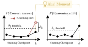 />
/>
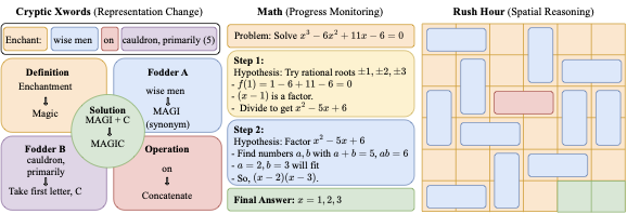 />
/>
Data
openR1 Math-220k and evaluate on
MATH-500 , ensuring no train/eval leakage
(App. 10.1). Answers are scored by
normalized exact match.Methods
Models and Training
<think> block and a concise final answer in <answer>, with
domain-level checks that invite reconsideration
(App. 10.2). Informed by
established strategies—zero-shot CoT, self-consistency, and reflection
routines —these prompts standardize mid-trace events as reasoning shifts
(Def. 1;
Alg. [alg:aha-moment]), enabling
consistent comparison across models, tasks, and checkpoints.
Model
Domain
Step 0
After
Step
$`\boldsymbol{\Delta}`$
Qwen2.5-1.5B
Xwords
7.69
10.00
950
+2.31
Qwen2.5-1.5B
Math
31.00
35.00
950
+4.00
Qwen2.5-1.5B
RHour
0.00
0.01
950
+0.01
Qwen2.5-7B
Math
61.60
66.40
500
+4.80
Llama 3.1-8B
Math
40.20
48.36
500
+8.16
Trace Collection and Annotation
<think> and a machine-checkable final response in
<answer>; token budgets and stop criteria are domain-specific and held
fixed across checkpoints.Uncertainty Measure and Intervention
<think> and <answer>
segments (e.g., $`\bar H_{\text{think}}`$ and $`\bar H_{\text{ans}}`$),
and use these sequence-level scores in downstream analyses.Results
RQ1: Reasoning Shifts & Model Accuracy
 /> = Qwen 2.5;
  /> =
Llama 3.1.
/> =
Llama 3.1.
Model
Domain
%Si, j
P(✓ ∣ Si, j = 0)
P(✓ ∣ Si, j = 1)
style="width:1em" />-1.5BXwords
1.22
0.096
0.201
Math
2.65
0.327
0.144
RHour
14.32
0.000
0.000
style="width:1em" />-7BMath
1.50
0.661
0.282
style="width:1em" />-8BMath
5.04
0.457
0.282
Overall
(Pooled)
6.31
0.290
0.066
 />
/>
RQ2: Training Stage & Temperature
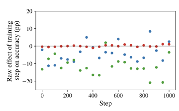 />
/>
 />
/>
temp_std).
Figure 6 shows the corresponding
per-$`T`$ raw pattern. On Xwords, the coefficient is positive but not
statistically distinguishable from zero ($`\mathrm{AME}{=}0.0326`$,
$`p{=}0.2595`$), despite a positive raw contrast
$`\Delta{=}{+}10.54`$pp. On Math, shifts are strongly harmful
($`\mathrm{AME}{=}{-}0.0831`$, $`p{=}2.68\times10^{-8}`$;
$`\Delta{=}{-}18.35`$pp). On RHour, shifts are frequent
($`\%S{=}14.32`$) but correctness is extremely low overall; accordingly,
the estimated effect is statistically detectable yet numerically
negligible ($`\mathrm{AME}{\approx}{-}0.0003`$,
$`p{=}2.72\times10^{-7}`$; $`\Delta{\approx}{-}0.02`$pp).
(a) Training
stage
Metric
Xword
Math
RHour
N
20,800
80,000
80,000
%S
2.433
2.166
11.449
p̂Y ∣ S = 1
0.0731
0.1691
0.0001
Δpp
−4.52
−11.83
+0.00
AME
−0.0311
−0.0615
0.0001
p
0.02742
1.55 × 10⁻⁴
≪ 10−6
(b)
Temperature
Metric
Xword
Math
RHour
N
83,200
320,000
320,000
%S
1.220
2.646
14.318
p̂Y ∣ S = 1
0.2010
0.1435
0.0000
Δpp
+10.54
−18.35
−0.02
AME
0.0326
−0.0831
−0.0003
p
0.2595
2.68 × 10⁻⁸
2.72 × 10⁻⁷
RQ3: Reasoning Shifts & Uncertainty
Metric
Xword
Math
RHour
All
traces
N
83,200
320,000
320,000
Δ (pp)
−6.24
−19.78
−0.02
coef(shift)
−1.49
−1.11
−22.76
p
0.123
2.25 × 10⁻⁷
≈ 0
High entropy (top
20%)
N
16,640
64,000
64,000
Δ (pp)
+0.63
−7.40
−0.03
coef(shift)
−0.04
−0.28
−22.48
p
0.904
0.739
≈ 0
Low entropy (bottom
80%)
N
66,560
256,000
256,000
Δ (pp)
−10.00
−22.88
−0.02
coef(shift)
−28.83
−1.14
−22.90
p
1.33 × 10−46249
4.96 × 10⁻⁷
≈ 0
Metric
Xword
Math
RHour
$`N`$ (paired samples)
83,200
320,000
320,000
$`\hat p_{\text{P1}}`$
0.0970
0.3221
0.000233
$`\hat p_{\text{P2}}`$
0.1015
0.4062
0.000363
$`\Delta`$ (pp)
$`+0.45`$
$`+8.41`$
$`+0.01`$
wins (P2 $`\uparrow`$)
5,380
50,574
100
wins (P1 $`\uparrow`$)
5,004
23,500
58
Discussion and Future Work
Limitations
Ethical Considerations
Acknowledgments
Experimental Setup and Data
<think>/<answer> formatting requirements and domain-specific
guardrails
(§10.2). Finally, we
summarize the GRPO training setup and per-domain hyperparameters
(§10.4; App. A.3). All of these
components are held fixed across checkpoints unless explicitly noted, so
that differences reported in the main text reflect changes in model
state rather than instruction drift or evaluation artifacts.Dataset Details
Cryptic Xwords.
Math.
openR1 Math-220k ; evaluation is on the
MATH-500 benchmark . Normalization
removes LaTeX wrappers, whitespace, and trivial formatting differences
(e.g., ‘$`1/2`$’ vs. ‘$`\frac{1}{2}`$’) before exact match.RHour.
Data release.
data/. We
also release the exact evaluation subsets on Hugging Face:
od2961/rush4-5-6-balanced and
od2961/Guardian-cryptonite-official-split.System-Level Prompts
Design goals.
<think> / </think> and
<answer> / </answer>), (b) enforce domain-specific guardrails
(e.g., enumeration and letter accounting for cryptics; canonical forms
for mathematics; regex-constrained action sequences for RHour), and (c)
build in a light-weight self-correction loop that triggers targeted
reconsideration when a check fails. The prompts below were held fixed
across checkpoints and temperatures (unless noted), ensuring that any
changes we observe arise from the model state rather than instruction
drift.Common scaffolding (all domains).
<think> and to place the
final object to be graded inside <answer> only. Tag separation
lets us (1) compute reasoning-shift features on the private trace
without leaking them into the final output, and (2) apply exact
validators to <answer>. To avoid verbosity that can mask errors,
prompts specify concise but complete derivations, a token budget, and
deterministic formatting. The reconsideration clause begins with a fixed
sentence (“Wait, we need to reconsider…”) to reliably demarcate pivot
points for analysis; however, our shift detector
(App. §11.1) additionally requires a
structural plan change, avoiding circularity from lexical cues alone.
Domain
Train ($`N`$)
Eval ($`N`$)
Cryptic Xwords
50,000
130
Math
220,000
500
RHour
180,000
500
Cryptic Xwords.
Math.
NO SOLUTION”) or underdetermined
(“I DON’T KNOW”), which reduces hallucinated specificity. The tag
split is enforced more strictly here to prevent the final answer from
appearing in <think> and to keep <answer> parsable for grading and
correctness metrics. The 750-token cap preserves headroom for multi-step
derivations while discouraging digressions that add entropy without
improving validity.RHour.
<answer> must match a
regular expression of move tokens
(^[A-Z][<>^v]\d+(,[A-Z][<>^v]\d+)*$). We add two verifiability
clauses: (i) the sequence must be optimal (minimum length), with
lexicographic tie-breaks to canonicalize multiple optimal plans; and
(ii) applying the sequence must achieve the goal ($`A`$ exits) in
exactly the declared number of moves. These guardrails allow us to
reject superficially plausible but illegal or suboptimal sequences and
to attribute improvements to better internal search rather than looser
grading.Configs and model release.
recipes/. We also release all trained models
(including checkpoints) on Hugging Face, listed in
Table [tab:hf-models].
Model
Domain
Hugging Face repository
Llama 3.1–8B
Math
https://huggingface.co/od2961/Llama-8B-Open-R1-GRPO-math-v1
Qwen 2.5–1.5B
Xwords
https://huggingface.co/od2961/Qwen2.5-1.5B-Open-R1-GRPO-Crosswords-v03
Qwen 2.5–1.5B
RHour
https://huggingface.co/od2961/Qwen2.5-1.5B-Open-R1-GRPO-carpark-v1
Qwen 2.5–7B
Math
https://huggingface.co/od2961/Qwen2.5-7B-Open-R1-GRPO-math-7b
Qwen 2.5–1.5B
Math
https://huggingface.co/od2961/Qwen2.5-1.5B-Open-R1-GRPO-math-v1Prompt Robustness & Evaluation
Robustness to system-prompt wording.
Qwen2.5-1.5B
(Open-R1 GRPO, trained on Math220k) on MATH-500 at decoding
temperature $`T{=}0`$, using randomized item order and a short prefilter
on input length (350 characters;
Table [tab:judge-reliability]). For
each epoch and prompt variant, we compute standard test accuracy and
then summarize the distribution across the five prompts. Across
variants, accuracy changes only modestly, and the qualitative
conclusions reported in the main text are unchanged. We therefore report
main results using the canonical system prompt shown above, and use the
prompt ensemble only to quantify prompt-induced variance.
Epoch
Mean accuracy
Std. across prompts
Range (min, max)
0 (pre)
31.8
0.8
(30.8, 33.2)
1 (ckpt 500)
38.8
1.2
(36.6, 40.0)
2 (ckpt 1000)
38.3
1.0
(36.8, 39.8)
3 (final)
40.2
0.7
(39.5, 41.4)
Reproducibility and evaluation.
Model Training (GRPO Setup)
Task / Model
Dataset
Key GRPO settings
OpenR1–Math–220k
grad_acc=64; epochs=3;
num_gens=4; max_prompt=512;
max_completion=750; reward=
pure_accuracy_math;
KL target 0.07, init_KL 3.0
OpenR1–Math–220k
grad_acc=32; epochs=3;
num_gens=4; max_prompt=450;
max_completion=750; reward=
pure_accuracy_math
OpenR1–Math–220k
grad_acc=8; epochs=3;
num_gens=4; max_prompt=450;
max_completion=750; reward=
pure_accuracy_math;
PPO clip 0.10
Guardian–Cryptonite (official split)
grad_acc=256; epochs=3;
num_gens=8;
return_reason=true;
max_reason=275; max_completion=320;
reward=
pure_accuracy (0/1 + shaping)
Rush 4/5/6–balanced
grad_acc=64; epochs=3;
num_gens=4;
return_reason=true;
max_prompt=3000; max_completion=300;
reward=
rush_solution_shaped
Overview.
<think> and a single, machine-checkable response in <answer> (See
App. §10.2).Rollout + training architecture.
accelerate+DeepSpeed ZeRO-3 for training. A
dedicated GPU hosts vLLM; the remaining GPUs run GRPO. Mixed precision
is bf16 for training; vLLM runs fp16. DeepSpeed is configured with
ZeRO-3, CPU offload for parameters/optimizer, and overlap-comm; the
accelerate configuration uses four to seven processes depending on
available devices.Domain–specific reward functions.
<answer> (strict 0/1) plus two
shaping signals: (i) a tiny “contains as a standalone word” bonus,
scaled by a tag factor (fraction of {<think>, </think>,
<answer>, </answer>} present), and (ii) a “Xwords accuracy” term
that linearly ramps with <think> length and is multiplied by the
same tag factor; optional enumeration checks reject length mismatches.<answer> are canonicalized (LaTeX/math normalization) and compared
for exact equality (0/1).Optimization and KL control.
Prompt templates and budgets.
<think>/<answer>
token budgets. This standardization lets the rewards remain reliable and
comparable across checkpoints and temperatures.Per-domain GRPO configurations.
DeepSpeed/Accelerate settings.
accelerate config sets bf16 mixed precision and num_processes
according to available training GPUs (vLLM occupies a dedicated device).Operational notes.
accelerate training. For the larger Qwen2.5-7B and
Llama 3.1-8B runs, we reserve two GPUs for vLLM to support
higher-throughput rollouts, with the remaining GPUs used for training.
Per-run environment/caching settings and health-checks follow the batch
script. The trainer logs per-step KL, policy/critic losses, and gradient
norms; checkpoints are saved every 50 steps and pushed locally/HF Hub
per config.Shift Detection, “Aha!” Detection, and Annotation
Algorithm: Detecting an “Aha!” Moment
Overview.
Estimating expected correctness.
\hat P_{\theta_k}(\checkmark \mid q_j)
\;=\;
\frac{1}{M}\sum_{m=1}^M R\!\big(\tau^{(m)}\big),
\qquad
R(\tau)\in\{0,1\}.\hat P_{\theta_k}(\checkmark \mid q_j,\; S_{q_j,k}{=}1)
\;=\;
\frac{\sum_{m=1}^M R(\tau^{(m)})\,\mathbb{1}[S(\tau^{(m)}){=}1]}
{\sum_{m=1}^M \mathbb{1}[S(\tau^{(m)}){=}1] + \epsilon},Detecting mid-trace shifts ($`S(\tau){=}1`$).
Prior stability (Step 2).
\widehat{\Pr}[S_{q_j,i}{=}1]
\;=\;
\frac{1}{M}\sum_{m=1}^M \mathbb{1}\!\big[S(\tau^{(m)}_{i}){=}1\big],Thresholds and statistical test (Step 3).
Decoding protocol.
Complexity and caching.
Edge cases and fallbacks.
Diagnostics.
Limitations.
Detecting Reasoning Shifts in Traces
<think> block. A
trace is labeled TRUE only if it exhibits both: (A) an explicit
lexical cue of reconsideration, and (B) a material revision of the
preceding plan (rejects/corrects an earlier hypothesis, switches method
or candidate, or resolves a contradiction). Otherwise the label is
FALSE.Annotation pipeline.
<think> and <answer> with a robust regex;
clamp <think> to 4,096 characters.<think> for any cue from a whitelist
(Table [tab:shift-cue-whitelist]).
If none is present, assign FALSE.<think> text,
problem/clue, and whitelist-prefiltered cue markers/position, with a
strict JSON schema for the verdict.Whitelist (lexical cues).
<think> text
(Table [tab:shift-cue-whitelist]),
covering common morphology and light paraphrase (e.g., “wait”, “hold
on”, “scratch that”, “I was wrong”, “misread”, “re-check”, etc.). Cues
are grouped semantically in the implementation (e.g.,
src/annotate/core/prefilter.py). A positive shift label is only
accepted when at least one explicit cue is present—either from the
prefilter or from cues the judge itself extracts.
Pauses & self–interruptions & wait, hold on/up, hang on, one/just
a second, give me a moment, pause, on second/further thought,
reconsider, rethink
Explicit pivots/corrections & actually, in fact, rather, instead
(of), let’s fix/correct that, correction:, to correct,
change/switch to, replace with, try/consider instead,
alternate/alternative, new candidate/answer/approach
Immediate reversals & no, that/this/it …, never mind/nvm,
disregard/ignore that, scratch/strike/forget that, I retract/take
it back, I stand corrected, not X but/rather Y
Error admissions & I was wrong / that’s wrong / incorrect, (my)
mistake, my bad, oops/whoops, apologies, erroneous
“Mis-*” failures & misread, miscount, miscalculate / calculation
error, misapply, misparse, misspell, misindex, misuse,
conflated, typo, off-by-one
Constraint/length mismatches (xword) & doesn’t fit/match
(length/pattern), letters don’t fit, pattern/length mismatch, too
many/few letters, wrong length, violates enumeration, doesn’t
parse, definition mismatch, not an anagram of, fodder mismatch
Contradictions/impossibility & contradiction, inconsistent,
can’t/cannot be, impossible, doesn’t make sense / add up, cannot
both, leads to a contradiction
Re–check / backtrack & recheck / double–check / check again,
re–evaluate / re–examine / upon review/reflection, backtrack, start
over/restart/reset/from scratch
“Prev X, but …” templates & I (initially/originally) thought …
but/however, previously … but/however, earlier … but/however,
however … correct/fix/instead/rather/change
Omission/oversight & I forgot/missed/overlooked/ignored, didn’t
notice, misremembered/misheard
Directional swaps & reversed / backwards, swapped, mixed up
Realization formulas & turns out, I (now) realize, on reflection,
after all
Failure templates & fails because, won’t work / not working, dead
endBlacklist (negatives & exclusions).
<think>. The judge prompt enforces these,
and our implementation forces FALSE when no explicit cue is present.Material-revision test (B).
before/after excerpts around the first cue to aid audits, and we only
accept a TRUE label when the judge’s JSON is parseable and
consistent with the excerpts. Otherwise we default to FALSE.Error handling, privacy, and rate limits.
<think>
segments before sending to the judge. Optional jitter (default
$`\le 0.25`$s) randomizes inter-call delays.Reproducibility.
stepNNN and path, and perform atomic rewrites. The detector is
content-idempotent: re-running will skip annotated lines and only fill
missing fields.Limitations.
LLM-as-a-Judge Protocol and Reliability
Bias mitigation.
Variant
System prompt summary
v1
Baseline strict judge: explicit cue (e.g., “wait”, “hold on”, “scratch that”, “contradiction”) AND a material revision; ignore hedging; judge only the <think> span.
v2
Audit <think> for change of course: cue + substantive revision required; ignore rhetorical connectives; conservative.
v3
“Corrects themselves mid-thought”: needs an explicit reconsideration cue and a replacement/fix of prior approach; ignore small edits/hedges.
v4
“Quality control”: cue + meaningful course change; minor tweaks/hedging are not shifts; judge only the <think> span.
v5
“Spot explicit change of mind”: cue + real update (reject/swap/repair); true shifts are rare.
Logged annotations.
Prefiltering.
Reliability (inter-prompt agreement).
Epoch
Judged $`N`$
Mean PO
Mean $`\kappa`$
0 (pre)
500
0.983
0.655
1 (ckpt 500)
500
0.986
0.759
2 (ckpt 1000)
500
0.988
0.770
3 (final)
500
0.988
0.719
Human validation.
Comparison
$`N`$
PO
Cohen’s $`\kappa`$
GPT–4o vs. human majority vote
20
0.900
0.794
Mean human–human (pairwise)
20
0.703
0.42
Mean LLM–human (pairwise)
20
0.758
0.51
Reproducibility.
Human Annotators Template
Annotator pool & consent.
IRB status.
Presentation & blinding.
<think> trace (with tags preserved;
traces clamped to 4096 characters). Model family, size, checkpoint,
temperature, and correctness signals were withheld.Labels & rubric.
Calibration & quality.
Agreement & adjudication.
Data handling.
<think> clamps), labels, and
aggregation scripts; any operational contact data (if present) were
excluded from the release.Task.
<think> trace for a math problem and answer: “Does
this <think> trace include a change in thinking?” Choices: Yes /
No.When to mark Yes.
When to mark No.
Quick checklist.
Worked Examples (Gold-Labeled)
Example A — YES
<think> trace <think>… computes with a wrong assumption, gets
$`360=90`$ (contradiction), then re-evaluates and sets up
$`\theta=(n-2)\cdot 180^\circ-1070^\circ`$ and solves under
$`0^\circ<\theta<180^\circ`$ …</think>Example B — NO
<think> trace <think>… $`\sqrt{27}=3\sqrt{3}`$$`\;\to\;`$
$`3/(3\sqrt{3})=1/\sqrt{3}`$$`\;\to\;`$ rationalize $`\to`$
$`\sqrt{3}/3`$ …</think>Example C — YES
<think> trace <think>… tries completing the square, finds it
awkward, then switches to factoring $`(x-7)(x+2)`$ …</think>Example D — NO
<think> trace <think>… uses the quotient rule; minor sign fix;
simplify …</think>Example E — YES
<think> trace <think>… first frames as permutations, then
switches to stars and bars: $`\binom{21}{1}=21`$ …</think>Example F — NO
<think> trace <think>… recalls $`n^{2}`$ $`\to`$
$`50^{2}=2500`$ …</think>Example G — YES
<think> trace <think>… starts prime factoring, then switches
to the Euclidean algorithm …</think>Example H — NO
<think> trace <think>… uses Vieta’s formulas $`\to`$ factor
$`\to`$ $`\{7,3\}`$ …</think>Question 1: Does this
<think> trace include a change in thinking? (Yes/No)a = 2^x \cdot 3^y \cdot 5^zb = 2^w \cdot 3^v \cdot 5^tx = 1, \quad y = 1, \quad z = 1w = x, \quad v = y, \quad t = zw = 1, \quad v = 1, \quad t = 1w + v + t = 31 + 1 + 1 = 3w = 1, \quad v = 1, \quad t = 1a = 2^1 \cdot 3^1 \cdot 5^1 = 2102^x \cdot 3^y \cdot 5^z < 2^{x'} \cdot 3^{y'} \cdot 5^{z'}Post Assessment
Additional Results and Robustness Checks
“Aha!” Moment Prevalence
How to read the heatmaps.
Cross-domain patterns.
Stricter gain thresholds.
Takeaway.
Formal Threshold Search
min_prior_steps=2),
and selected the “best” configuration according to the script’s default
ranking (maximize the bootstrap lower CI bound for the mean gain; ties
broken by prevalence and mean gain).
Table [tab:formal-threshold-search-q15b]
reports the best row per root. We report mean gain as
$`100\cdot\mathbb{E}[\hat P(\checkmark\mid S{=}1)-\hat P(\checkmark)]`$
in percentage points (pp), with a 95% bootstrap CI over flagged pairs;
entries are “–” when no events are found or when $`N`$ is too small to
form a stable CI.
Domain
$`T`$
$`\boldsymbol{\delta_1}`$
$`\boldsymbol{\delta_2}`$
$`\boldsymbol{\delta_3}`$
events/pairs
prev (%)
gain (pp)
CI (pp)
Math
0
1/8
1/8
$`\epsilon`$
8/16000
0.05
+0.00
[+0.00, +0.00]
Math
0.05
2/8
2/8
$`\epsilon`$
41/16000
0.26
-2.74
[-5.79, -0.30]
Math
0.3
2/8
2/8
$`\epsilon`$
43/10000
0.43
-2.62
[-4.65, -1.16]
Math
0.7
2/8
2/8
$`\epsilon`$
92/16000
0.57
+1.22
[-1.77, +4.76]
Xwords
0
0
0
$`\epsilon`$
0/3120
0.00
–
–
Xwords
0.05
1/8
1/8
$`\epsilon`$
3/3120
0.10
+0.00
[+0.00, +0.00]
Xwords
0.3
1/8
1/8
$`\epsilon`$
7/3120
0.22
+0.00
[+0.00, +0.00]
Xwords
0.7
2/8
2/8
$`\epsilon`$
18/3120
0.58
+0.00
[+0.00, +0.00]
RHour
0
1/8
1/8
$`\epsilon`$
1/503
0.20
+0.00
–
RHour
0.05
1/8
1/8
$`\epsilon`$
1/498
0.20
-0.07
–
RHour
0.3
1/8
1/8
$`\epsilon`$
7/498
1.41
-0.01
[-0.01, +0.00]
RHour
0.7
1/8
1/8
$`\epsilon`$
18/513
3.51
-0.01
[-0.02, -0.00]
Takeaway.
Qwen-7B and Llama-8B Regressions
/>
Step and Temperature Analysis
 />
/>
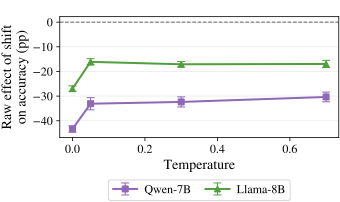 />
/>
(a) Training stage
(fixed T = 0.7)
Metric
Qwen2.5–7B
Llama 3.1–8B
Combined
N
40,000
40,000
40,000
%S
1.37
6.54
3.89
p̂Y ∣ S = 1
0.3467
0.2709
0.2846
Δ (pp)
−30.39
−17.68
−26.97
AME
−0.0841
−0.0688
−0.1706
p
4.38 × 10⁻⁴
6.7 × 10⁻¹¹
5.93 × 10−42
(b) Temperature
(temps pooled, steps ≤ 450)
Metric
Qwen2.5–7B
Llama 3.1–8B
Combined
N
160,000
160,000
320,000
%S
1.50
5.04
3.26
p̂Y ∣ S = 1
0.2821
0.2816
0.2818
Δ (pp)
−37.85
−17.56
−27.94
AME
−0.0833
−0.0529
−0.1457
p
4.89 × 10⁻⁶
2.25 × 10⁻⁵
2.83 × 10⁻²²
Uncertainty Analysis
Shift prevalence vs. entropy.
\texttt{shift} \sim \texttt{C(problem)} + \texttt{std\_entropy}.Entropy-stratified shift effects on accuracy.
Metric
Qwen2.5–7B
Llama 3.1–8B
Combined
All traces (temps
pooled, steps ≤ 450)
N
160,000
160,000
320,000
Δ (pp)
−44.43
−14.83
−33.69
p
1.32 × 10⁻⁴
0.6973
0.001725
High entropy (top
20%)
N
32,000
31,757
63,763
Δ (pp)
−22.03
−8.93
−10.30
p
0.06963
0.7834
0.001017
Low entropy (bottom
80%)
N
128,000
127,027
255,021
Δ (pp)
−48.87
−14.23
−38.86
p
1.44 × 10⁻⁴
0.7221
0.01824
Forced reconsideration as a separate mechanism.
Metric
Qwen2.5–7B
Llama 3.1–8B
$`N`$
14,176
222,658
$`\hat p_{\text{P1}}`$
0.5509
0.4416
$`\hat p_{\text{P2}}`$
0.6107
0.3997
$`\Delta`$ (pp)
$`+5.97`$
$`-4.19`$
wins (P2 $`\uparrow`$)
2,156
27,106
wins (P1 $`\uparrow`$)
1,309
36,439
Entropy-Gated Interventions with Multiple Cues
Cue
$`\beta`$ (std. ent.)
OR
OR$`_{1\sigma}`$
C1
0.79
3.64
2.21
[0.59, 1.00]
[2.60, 5.09]
[1.80, 2.72]
C2
0.86
4.32
2.36
[0.65, 1.07]
[3.03, 6.17]
[1.92, 2.91]
C3
0.91
4.09
2.49
[0.71, 1.12]
[2.98, 5.62]
[2.03, 3.06]
Reasoning Shifts at Scale
Experimental setup.
<think> and <answer> tags),Shift detection.
Results.
Model
$`T`$
# Problems
% Shifts (count)
$`P(\checkmark \mid S{=}1)`$
DeepSeekR1
0
500
0.60% (3)
0.67
DeepSeekR1
0.05
500
0.40% (2)
0.50
GPT4o
0
500
3.00% (15)
0.60
GPT4o
0.05
500
2.20% (11)
0.18
Interpretation.
Data release.
Model
Dataset (Hugging Face)
GPT4o
od2961/gpt4o-math500-t0
GPT4o
od2961/gpt4o-math500-t005
DeepSeekR1
od2961/deepseek-r1-math500-t0
DeepSeekR1
od2961/deepseek-r1-math500-t005Alternate Shift Detectors
Detector variants.
formal). The strict criterion in
Def. 1, which requires (i) prior
failure, (ii) prior stability, and (iii) a performance gain on
traces with a detected shift.gpt). GPT-4o marks a shift when it observes
an explicit cue of reconsideration together with a material change
in reasoning strategy
(App. 11.2).words). A looser detector that flags a
shift whenever the <think> trace contains at least one cue phrase
from our whitelist, regardless of whether the subsequent reasoning
reflects a genuine plan pivot.Metrics.
Domain
Detector
$`\%S`$
$`\hat p_{Y\mid S=1}`$
$`\hat p_{Y\mid S=0}`$
$`\Delta\%`$
$`\mathrm{AME}`$ ($`p`$)
Xword
formal
0.0008
0.0000
0.1181
$`-11.81`$
$`-0.1181`$ (0)
gpt
0.0010
0.0400
0.1181
$`-7.81`$
$`-0.0651`$ (0.05095)
words
0.0013
0.0312
0.1182
$`-8.69`$
$`-0.0712`$ (0.04761)
Math
formal
0.0008
0.0215
0.3006
$`-27.91`$
$`+0.0275`$ (0.8201)
gpt
0.0030
0.1622
0.3008
$`-13.87`$
$`-0.1086`$ ($`7.80\times10^{-6}`$)
words
0.0120
0.2606
0.3009
$`-4.03`$
$`-0.0469`$ (0.002153)
RHour
formal
0.0023
0.0000
0.0001
$`-0.01`$
$`-0.0001`$ (0)
gpt
0.0026
0.0000
0.0001
$`-0.01`$
$`-0.0001`$ (0)
words
0.0060
0.0000
0.0001
$`-0.01`$
$`-0.0001`$ (0)
Takeaways.
words) identifies shifts in at most $`1.2\%`$ of
Math traces and $`0.6\%`$ of RHour traces; the formal Aha
criterion is stricter still.formal detector, where the estimate is small and
statistically indistinguishable from zero ($`p{=}0.82`$). In
Math, both the GPT-based and lexical
detectors show statistically significant negative AMEs.Aha definition, the rubric-guided GPT detector, or a
lexical cue heuristic, mid-trace shifts are rare and generally harm
correctness rather than help it.Supplementary Figures & Tables
Overview.
Training-stage effects at other decoding temperatures
Training stage at
fixed decoding temperature T = 0.0
Metric
Xword
Math
RHour
N
20,800
80,000
80,000
%S
0.947
1.866
14.679
p̂Y ∣ S = 1
0.3655
0.0683
0.0000
Δpp
+28.24
−23.64
−0.04
AME
0.0027
−0.0044
−0.0001
p
6.89 × 10⁻³⁵
1.19 × 10−67
0.999
Training stage at
fixed decoding temperature T = 0.05
Metric
Xword
Math
RHour
N
20,800
80,000
80,000
%S
0.851
1.854
15.386
p̂Y ∣ S = 1
0.3390
0.1382
0.0000
Δpp
+25.41
−18.56
−0.05
AME
0.0022
−0.0034
−0.0001
p
1.94 × 10⁻²⁶
2.0 × 10−47
0.999
Training stage at
fixed decoding temperature T = 0.3
Metric
Xword
Math
RHour
N
20,800
80,000
80,000
%S
0.649
4.696
15.759
p̂Y ∣ S = 1
0.2593
0.1637
0.0000
Δpp
+16.28
−23.01
−0.01
AME
0.0011
−0.0108
−0.0000
p
1.93 × 10⁻⁹
1.58 × 10−158
0.999
Training-stage effects at other decoding temperatures (Qwen-7B and Llama-8B)
Training stage at
fixed decoding temperature T = 0
Metric
Qwen2.5-7B
Llama3.1-8B
N
40,000
40,000
%S
2.538
2.418
p̂Y ∣ S = 1
0.2039
0.1607
Δpp
−45.10
−27.18
AME
−0.0659
−0.0597
p
0.03314
0.04043
Training stage at
fixed decoding temperature T = 0.05
Metric
Qwen2.5-7B
Llama3.1-8B
N
40,000
40,208
%S
0.853
5.710
p̂Y ∣ S = 1
0.3284
0.3319
Δpp
−34.06
−14.82
AME
−0.0401
−0.0436
p
0.07879
0.007971
Training stage at
fixed decoding temperature T = 0.3
Metric
Qwen2.5-7B
Llama3.1-8B
N
40,000
40,192
%S
1.248
5.576
p̂Y ∣ S = 1
0.3387
0.2945
Δpp
−32.91
−17.44
AME
−0.0788
−0.0540
p
2.91 × 10⁻⁴
4.4 × 10⁻⁵
Formal “Aha!” moments across decoding temperatures
Metric
Crossword
Math
RHour
T = 0.0
N
20,800
80,000
80,000
%S
0.471
0.462
0.000
p̂Y ∣ S = 1
0.0816
0.0000
–
Δpp
−0.42
−30.17
–
AME
−0.0000
−0.0014
–
p
0.883
0.999
–
T = 0.05
N
20,800
80,000
80,000
%S
0.212
0.299
0.000
p̂Y ∣ S = 1
0.0000
0.0251
–
Δpp
−8.72
−29.62
–
AME
−0.0002
−0.0009
–
p
0.999
1.92 × 10⁻¹²
–
T = 0.3
N
20,800
80,000
80,000
%S
0.312
0.475
0.000
p̂Y ∣ S = 1
0.0000
0.0211
–
Δpp
−9.78
−36.36
–
AME
−0.0003
−0.0017
–
p
0.999
4.17 × 10⁻²¹
–
T = 0.7
N
20,800
80,000
80,000
%S
1.438
0.364
8.191
p̂Y ∣ S = 1
0.0067
0.0241
0.0002
Δpp
−11.22
−26.17
+0.01
AME
−0.0016
−0.0010
0.0000
p
2.41 × 10⁻⁵
3.25 × 10⁻¹³
0.461
Formal “Aha!” moments across decoding temperatures (Qwen-7B and Llama-8B)
Metric
Qwen2.5-7B
Llama3.1-8B
T = 0
N
40,000
40,000
%S
0.362
0.832
p̂Y ∣ S = 1
0.0621
0.0449
Δpp
−58.35
−38.42
AME
+0.0541
+0.0112
p
0.6627
0.815
T = 0.05
N
40,000
40,000
%S
0.048
0.090
p̂Y ∣ S = 1
0.0000
0.0278
Δpp
−66.64
−44.42
AME
−0.3735
+0.1626
p
1.84 × 10−135441
0.2839
T = 0.3
N
40,000
40,000
%S
0.045
0.109
p̂Y ∣ S = 1
0.0000
0.0000
Δpp
−66.40
−45.97
AME
−0.4970
−0.4114
p
8.64 × 10−65910
3.13 × 10−95446
T = 0.7
N
40,000
40,000
%S
0.022
0.073
p̂Y ∣ S = 1
0.0000
0.0357
Δpp
−64.66
−40.08
AME
−0.5572
+0.1937
p
4.7 × 10−54940
0.1153
Additional Temperature Ablations
Qualitative review of formal “Aha!” Moments
Math.
min_prior_steps=2.Xword.
min_prior_steps=2.RHour.
min_prior_steps=2. Because RHour accuracies are near zero in these
stored outputs, we found too few events satisfying a positive gain
constraint; we therefore omit the gain threshold for this qualitative
inspection.Triggered reconsideration under uncertainty
Entropy-gated gains (nonparametric stratification).
Domain
Bucket
$`N`$
$`\hat p_{\text{P1}}`$ (%)
$`\hat p_{\text{P2}}`$ (%)
$`\Delta`$ (pp)
Xword
all
99,840
9.65
10.15
+0.49
Xword
high
19,969
8.56
9.59
+1.04
Xword
low
79,871
9.93
10.29
+0.36
Math
all
464,000
32.70
40.43
+7.74
Math
high
92,800
19.70
35.09
+15.38
Math
low
371,200
35.94
41.77
+5.82
RHour
all
331,120
0.023
0.036
+0.013
RHour
high
66,224
0.027
0.023
-0.005
RHour
low
264,896
0.022
0.039
+0.017
Overall
all
894,960
18.04
22.11
+4.07
Overall
high
178,993
11.18
19.27
+8.09
Overall
low
715,967
19.75
22.82
+3.07
Entropy as a continuous predictor (regression).
Domain
$`N`$
$`\beta_{\mathrm{ent}}`$
$`\mathrm{OR}_{1\sigma}`$
$`p`$
Xword
99,840
$`-0.033`$
$`0.97`$
0.091
Math
464,000
$`+0.019`$
$`1.02`$
0.146
RHour
331,120
$`-0.407`$
$`0.67`$
$`2.36\times10^{-119}`$
Pass-2 entropy regression for larger models.
Group
$`N`$
$`\beta_{\mathrm{ent}}`$
$`\mathrm{OR}_{1\sigma}`$
$`p`$
Qwen2.5-7B
63,404
$`+0.012`$
$`1.01`$
0.7586
Llama3.1-8B
102,232
$`-0.075`$
$`0.93`$
0.005146
Pass-2 accuracy conditional on detected shifts (additional summary)
Experiment
$`T`$
$`N`$
$`\%S`$
$`P_2(\checkmark\mid S{=}1)`$
$`P_2(\checkmark\mid S{=}0)`$
$`\Delta_2`$ (pp)
Qwen2.5–1.5B (all domains)
all
723,200
7.65
3.95
20.42
$`-16.47`$
Qwen2.5–7B (Math)
0.0
39,080
2.54
25.62
67.10
$`-41.47`$
Qwen2.5–7B (Math)
0.05
2,768
0.85
13.64
64.20
$`-50.57`$
Qwen2.5–7B (Math)
0.3
1,104
1.25
30.77
57.79
$`-27.03`$
Qwen2.5–7B (Math)
0.7
20,180
1.37
45.07
64.73
$`-19.66`$
Llama 3.1–8B (Math)
0.0
14,728
2.42
32.94
36.67
$`-3.74`$
Llama 3.1–8B (Math)
0.05
28,808
5.71
24.67
37.20
$`-12.53`$
Llama 3.1–8B (Math)
0.3
30,240
5.58
27.78
40.19
$`-12.41`$
Llama 3.1–8B (Math)
0.7
28,376
6.54
28.01
42.36
$`-14.35`$
& & &
& & &
& & &
& &
& &
& &
Release and Artifacts
Repository.
Contact.
problem: If $`\arccos x + \arccos 2x + \arccos 3x = \pi,`$ then
$`x`$ satisfies a cubic polynomial of the form
$`ax^3 + bx^2 + cx + d = 0,`$ where $`a,b,c,d`$ are integers and
$`a\neq 0`$. Find the smallest possible value of $`|a|+|b|+|c|+|d|`$.
step: 100n_samples: 8shift_rate: 0.125freq_correct:
0.125**$`p(\checkmark\mid S{=}1)`$:** 1.000gain: +87.50 pp
Shift cue: contradictionStrategy shift: propose $`x`$
$`\rightarrow`$ feasibility check $`\rightarrow`$ backtrack / replan
Shift excerpt (PASS-1): [SHIFT at “However, substituting $`x=0`$
… does not satisfy”]
markers: contradiction
…x = 0. However, substituting $`x = 0`$ into the original equation
does not satisfy it becausecontradicts $`\pi`$. Therefore, let’s
consider other values of $`x`$ that might work. We need to solve the
system of equations formed …
PASS-1 <answer>: $`-1/27`$
problem: Let $`a,b,c,d`$ be positive real numbers such that
$`a+b+c+d=1`$. Find the minimum value of
$`\frac{1}{a}+\frac{1}{b}+\frac{4}{c}+\frac{16}{d}`$.
step: 850n_samples: 8shift_rate: 0.125freq_correct:
0.125**$`p(\checkmark\mid S{=}1)`$:** 1.000gain: +87.50 pp
Shift cue: insteadStrategy shift: dead-end/degenerate reasoning
$`\rightarrow`$ switch to AM-GM template
Shift excerpt (PASS-1): [SHIFT at “Instead, let’s consider …
AM-GM”]
markers: instead
…we get:\frac{1}{a} + \frac{1}{b} + \frac{4}{c} + \frac{16}{d} = \infty.
PASS-1 <answer>: $`64`$
problem: Let $`x_1,x_2,x_3,y_1,y_2,y_3`$ be real numbers such that\begin{align*}
(x_1 - x_2)^2 + (y_1 - y_2)^2 &= 9, \\
(x_1 - x_3)^2 + (y_1 - y_3)^2 &= 16, \\
(x_2 - x_3)^2 + (y_2 - y_3)^2 &= 25.
\end{align*}
step: 400n_samples: 8shift_rate: 0.125freq_correct:
0.125**$`p(\checkmark\mid S{=}1)`$:** 1.000gain: +87.50 pp
Shift cue: insteadStrategy shift: direct determinant
manipulation $`\rightarrow`$ switch to “consider determinant itself”
(reframe)
Shift excerpt (PASS-1): [SHIFT at “Instead, we will consider the
determinant itself …”]
markers: instead
…However, finding the determinant directly from these equations might
not be straightforward.Instead, we will consider the determinant
itself and see if we can simplify our approach. $`\cdots`$
PASS-1 <answer>: 144
problem: A hexagon is inscribed in a circle (diagram omitted). What
is the measure of $`\alpha`$, in degrees?
step: 100n_samples: 8shift_rate: 0.125freq_correct:
0.125**$`p(\checkmark\mid S{=}1)`$:** 1.000gain: +87.50 pp
Shift cue: howeverStrategy shift: algebra gives invalid angle
$`\rightarrow`$ constraint check (angle must be positive)
$`\rightarrow`$ sign correction
Shift excerpt (PASS-1): [SHIFT at “However, since $`\alpha`$ …
should be positive”]
markers: however
…Simplifying, $`\alpha + 110^\circ = 70^\circ`$, leading to
$`\alpha = -40^\circ`$. However, since $`\alpha`$ represents an angle
within the circle, it should be positive. $`\cdots`$
PASS-1 <answer>: $`40`$
problem: Compute $`\sin^3 18^\circ + \sin^2 18^\circ`$.
step: 900n_samples: 8shift_rate: 0.125freq_correct:
0.125 $`\mathbf{p}(\checkmark\mid S{=}1)`$: 1.000gain: +87.50
pp
Shift cue: insteadStrategy shift: failed analytic attempt
$`\rightarrow`$ abandon/switch to numerical/other-method talk (search
collapse)
Shift excerpt (PASS-1): [SHIFT at “Instead, let’s try solving
numerically …”]
markers: instead
…Since $`\sqrt{5} > 3`$, $`y = \frac{1}{2}`$ does not satisfy the
equation.Instead, let’s try solving numerically or by another
method. $`\cdots`$
PASS-1 <answer>: $`-1/8`$
problem: Front of ship; bend (3)
step: 1000n_samples: 8shift_rate: 0.125freq_correct:
0.125**$`p(\checkmark\mid S{=}1)`$:** 1.000gain: +87.50 pp
Shift cue: doesn’t fitStrategy shift: definition mismatch
$`\rightarrow`$ reinterpret “front of ship” $`\rightarrow`$ BOW
Shift excerpt (PASS-1): [SHIFT at “However, considering … ship’s
front …”]
markers: doesn’t fit
…the definition does not fit directly. However, considering the
context of a ship’s front, …
PASS-1 <answer>: BOW
problem: Clue: Celebrity from stare losing tail (4)Gold: STAR
step: 300n_samples: 8shift_rate: 0.125freq_correct:
0.125p_correct_given_shift: 1.000gain: +87.50 pp
Shift excerpt (PASS-1): [SHIFT: doesn’t fit]Strategy shift: length
mismatch $`\rightarrow`$ simplify transformation
markers: doesn’t fit
…Attempt with “TILL”: Definition: “Celebrity” could be fitting given the
context, but the length is still too much.
This seems too long and doesn’t fit easily into the 4-letter constraint.
Wordplay: STARE loses its TAIL → STAR. PASS-1 <answer>: STAR
problem: Clue: Shoe liner at home on fish (6)Gold: INSOLE
step: 550n_samples: 8shift_rate: 0.250freq_correct:
0.250p_correct_given_shift: 0.500gain: +25.00 pp
Shift excerpt (PASS-1): [SHIFT: doesn’t fit / re-evaluate]Strategy
shift: reject homophone $`\rightarrow`$ switch to charade
markers: doesnt fit, re-evaluate
…Homophone? (“shoe” sounds like “soe”) - Doesn’t fit here
Candidate attempt (WRONG PATH): - HIDDEN: No hidden indicator present -
WRONG PATH: Consider other indicators
Re-evaluate as CHARADES: IN (“at home”) + SOLE (“fish”) → INSOLE.
Accounting: INSOLE letters: I N S O L E (6). Definition “Shoe liner”
fits. Enumeration (6) OK.
Final answer: INSOLE
PASS-1 <answer>: INSOLE
problem: Clue: Frighten when energy enters scar (5)Gold: SCARE
step: 900n_samples: 8shift_rate: 0.250freq_correct:
0.125p_correct_given_shift: 0.500gain: +37.50 pp
Shift excerpt (PASS-1): [SHIFT: rethink / re-evaluate]Strategy shift:
failed parse $`\rightarrow`$ substitution re-parse
markers: rethink, re-evaluate
…Device matches, but there’s no indication that it should be considered
an abbreviation. Candidate attempt (wrong path): — fails definition, so
we mustrethink. Re-evaluate as SUBSTITUTION: SCARE → SCARE. Accounting:
SCARE letters: S C A R E (5). Definition “Frighten” fits. Enumeration
(5) OK.
PASS-1 <answer>: SCARE
problem: example_id: idx_101Gold: [’Cv2’, ’A>1’]
step: 950n_samples: 8shift_rate: 1.000freq_correct:
0.000**$`p(\checkmark\mid S{=}1)`$:** 0.000gain: +0.00 pp
Shift cue: hang onStrategy shift: attempt $`\rightarrow`$ detect
blocker $`\rightarrow`$ replan with enabling move
Shift excerpt (PASS-1): [SHIFT at “Hang on…”]
markers: hang on
…S1: E>1 $`\rightarrow`$ GOAL$`\times`$ (blocked by D). Hang on…
S2: Fv1,E>1 $`\rightarrow`$ GOAL$`\checkmark`$ (all valid sequences
pass this check).
PASS-1 <answer>: Fv1,E>1
problem: example_id: idx_109Gold: [’Cv1’, ’Cv1’, ’A>2’]
step: 600n_samples: 8shift_rate: 0.375freq_correct:
0.000**$`p(\checkmark\mid S{=}1)`$:** 0.000gain: +0.00 pp
Shift cue: check againStrategy shift: local fix $`\rightarrow`$
explicit verification pass $`\rightarrow`$ continue search
Shift excerpt (PASS-1): [SHIFT at “Check again …”]
markers: check again
…Move B >1 to avoid collision with D. Check again for collisions
after moving B: No more collisions detected.…
PASS-1 <answer>: C>1,E>1
📊 논문 시각자료 (Figures)
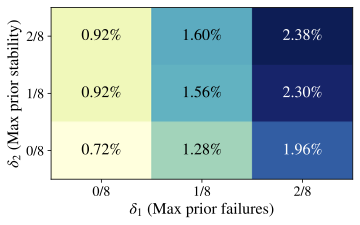
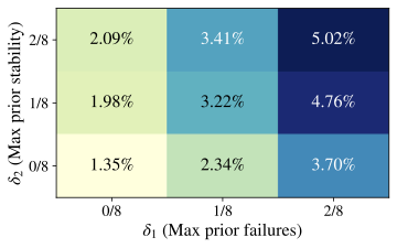
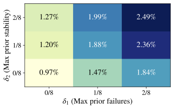
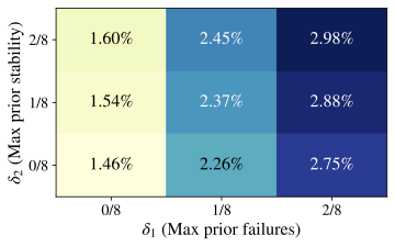
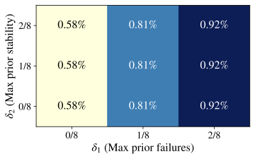
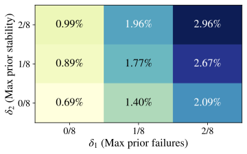
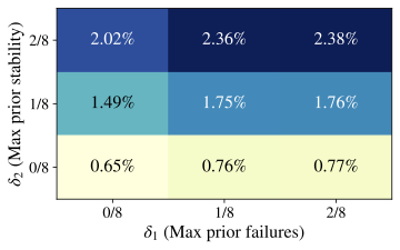
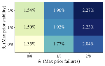
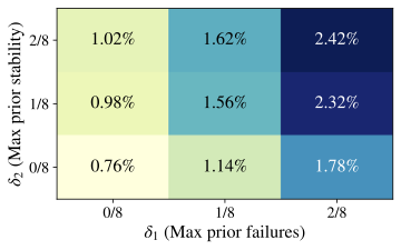
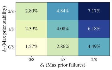
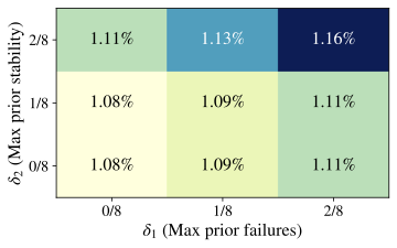


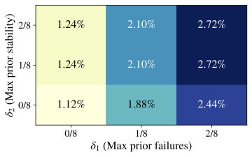

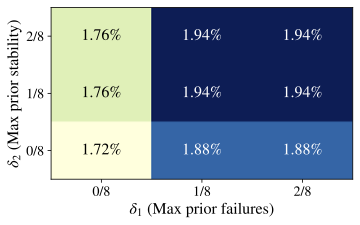
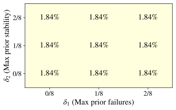
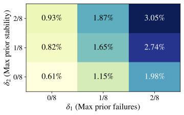
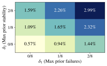

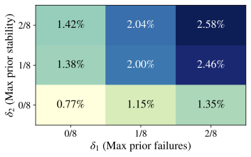

A Note of Gratitude
The copyright of this content belongs to the respective researchers. We deeply appreciate their hard work and contribution to the advancement of human civilization.-
Formal “Aha!” events are defined over problem–checkpoint pairs $`(q_j,k)`$ (i.e., a checkpoint-level comparison for a fixed problem), not over individual sampled traces. ↩︎
-
In R-style notation, $`\texttt{correct} \sim \texttt{shift}.`$
correctis a binary outcome, andshiftis a binary indicator for an annotator-labeled reasoning shift. The pooled regression aggregates all test-set traces across Crossword, Math, and RHour. ↩︎ -
In R-style notation: $`\texttt{correct} \sim \texttt{C(problem)} + \texttt{step\_std} + \texttt{shift}.`$
correctis a binary outcome;C(problem)are problem fixed effects;step_stdis the standardized checkpoint index. ↩︎ -
R-style notation: $`\texttt{correct} \sim \texttt{C(problem)} + \texttt{temp\_std} + \texttt{shift}.`$
temp_stdis the standardized decoding temperature. ↩︎ -
In R-style notation: $`\texttt{shift} \sim \texttt{C(problem)} + \texttt{std\_entropy}.`$ Here
shiftis a binary indicator for a reasoning shift,C(problem)denotes problem fixed effects, andstd_entropyis the within-domain $`z`$-scored pass-1 sequence entropy. We estimate a Binomial(logit) GLM with cluster-robust SEs at the problem level. ↩︎ -
Within each domain, we split at the 80th percentile of sequence entropy and fit a Binomial(logit) GLM predicting
correctfromshiftwith problem fixed effects and covariates. We report both regression and raw contrasts for interpretability. ↩︎ -
In R-style notation: $`\texttt{correct} \sim \texttt{entropy\_std} + \texttt{baseline\_correct} + \texttt{C(problem)}.`$ Here
entropy_stdis the within-domain standardized sequence-level entropy defined in §5.3. ↩︎