From Building Blocks to Planning Multi-Step Spatial Reasoning in LLMs with Reinforcement Learning
📝 Original Paper Info
- Title: From Building Blocks to Planning Multi-Step Spatial Reasoning in LLMs with Reinforcement Learning- ArXiv ID: 2512.24532
- Date: 2025-12-31
- Authors: Amir Tahmasbi, Sadegh Majidi, Kazem Taram, Aniket Bera
📝 Abstract
Spatial reasoning in large language models (LLMs) has gained increasing attention due to applications in navigation and planning. Despite strong general language capabilities, LLMs still struggle with spatial transformations and multi-step planning in structured environments. We propose a two-stage approach that decomposes spatial reasoning into atomic building blocks and their composition. First, we apply supervised fine-tuning on elementary spatial transformations, such as rotation, translation, and scaling, to equip the model with basic spatial physics. We then freeze this physics-aware model and train lightweight LoRA adapters within the GRPO framework to learn policies that compose these building blocks for multi-step planning in puzzle-based environments, in a closed-loop manner. To support this pipeline, we synthesize an ASCII-art dataset and construct a corresponding ASCII-based reinforcement learning environment. Our method consistently outperforms baselines, including the generic backbone, physics-aware model, and end-to-end RL models, under both Dynamic environments with explicit state updates and Static environments where the model must rely on its internal state across steps. In addition, the proposed approach converges faster and exhibits more stable training compared to end-to-end reinforcement learning from scratch. Finally, we analyze attention patterns to assess whether fine-tuning induces meaningful improvements in spatial understanding.💡 Summary & Analysis
1. **Enhanced Spatial Understanding Through Machine Learning**: This research presents methods to enhance a model's ability to understand and solve complex spatial relationships by first learning basic physical transformations and then using these as building blocks for more intricate problems. It’s akin to how a beginner driver learns basic driving maneuvers before handling complex traffic situations safely.-
Two-Stage Learning Methodology: The study introduces a two-stage learning approach where the model initially learns foundational transformations, followed by reinforcement learning that teaches it to combine these basics into solutions for larger problems. This is similar to how a chef first masters the preparation of basic ingredients and then uses them to create diverse recipes.
-
Performance Improvement and Faster Convergence: The proposed method shows better performance than baseline models and converges faster during reinforcement learning. It’s like an athlete improving their basic skills and using those improvements as a foundation for mastering more complex techniques, thereby enhancing overall game performance.
📄 Full Paper Content (ArXiv Source)
Introduction
Spatial reasoning and understanding represent the capability to reason about spatial relationships of objects and transformations in an environment. This includes understanding relative positions, orientations, distances, and the effects of actions that modify spatial configurations. With the recent advancements of LLMs and VLMs in a wide variety of tasks, such as math reasoning and vision–language understanding , their spatial reasoning capabilities have gained more attention, with applications such as robotics and language navigation tasks . However, their abilities in spatial reasoning have not yet been widely explored . Spatial reasoning tasks can often be mapped into several domains, some of which focus on linguistic and natural language scenarios , as well as puzzle-based settings such as mazes , Rubik’s Cube , and Sokoban , where the model needs to understand the spatial relationships among objects to solve the task. In puzzle-based settings, language models are empowered by several techniques. One category involves using an external module as a solver, with the LLM acting as an action recommender or reasoning candidate generator. The external module can be heuristic-based, such as BFS or DFS in Tree of Thoughts (ToT) , or learning-based approaches, such as XoT, which leverages pretrained reinforcement learning and Monte Carlo Tree Search (MCTS) , or Q-learning . Another category of approaches focuses on the model itself. One direction aims to change the model’s behavior through prompting, such as Visualization-of-Thought (VoT) , which elicits spatial reasoning in LLMs by visualizing their reasoning traces and guiding subsequent reasoning steps. Another approach, presented in , is inspired by DeepSeek-R1 and is based on supervised fine-tuning the model on solution traces, and then applying GRPO to further refine reasoning steps on the same task and structure.
In this work, we focus on spatial reasoning in a puzzle-based setting, where an agent must transform an initial spatial configuration into a target configuration through a sequence of discrete actions. We propose a novel approach that decomposes spatial understanding into a set of building blocks, consisting of atomic transformations such as rotating a shape by $`90^\circ`$ or translating it one grid cell upward. We first apply supervised fine-tuning to enable the model to learn these basic physical transformations. After this stage, the physics-aware model is kept frozen, and reinforcement learning is applied on top of it by introducing lightweight adapter layers that learn a policy for composing these building blocks as primitives to reach a target spatial configuration from a given starting point. An overview of our approach is shown in Figure 1.
For the supervised fine-tuning stage, we synthesize a dataset of 12k tasks spanning three transformation categories, translation, rotation, and scaling, which is used to fine-tune the Qwen2.5-1.5B-Instruct model . In the subsequent reinforcement learning stage, the physics-aware model is embedded directly in the reinforcement learning loop within a multi-step, compositional environment. Reinforcement learning is applied via GRPO to optimize lightweight LoRA adapter layers on top of the frozen backbone, enabling the model to learn policies over sequences of atomic spatial operations through repeated interaction with the environment. We evaluate our approach against several baselines, including the generic Qwen2.5-1.5B-Instruct model, the physics-aware model trained only with supervised fine-tuning, and a Qwen model trained directly with GRPO reinforcement learning. All models are tested on unseen spatial reasoning tasks under two settings: one where the environment map is updated after each action, and one where the map remains fixed. Our results show that the proposed method achieves higher rewards than all baselines across both settings and converges faster during reinforcement learning. Although the physics-aware model trained only with supervised fine-tuning underperforms the generic backbone on the final task, it provides a stronger prior for reinforcement learning, leading to substantially better performance after GRPO optimization. Finally, we conduct ablation studies on attention layers to analyze whether the learned improvements reflect genuine spatial understanding.
 />
/>
Related Work and Background
Spatial Reasoning in LLMs
Spatial reasoning in large language models has been studied across a range of domains. One line of research focuses on textual inputs, where spatial semantics are embedded in text and models are required to reason about relative spatial relations, such as left of or right of, expressed through language . A further step is explored in natural language navigation tasks, where, given a sequence of textual instructions, the model must maintain an implicit spatial state and track its position over multiple steps. In these settings, spatial understanding is inferred from sequential language instructions rather than from explicit spatial representations such as symbolic layouts . Recent efforts explore symbolic environments, particularly ASCII-art representations, which bridge the gap between text and image modalities in applications such as level generation . Results show that large language models are capable of recognizing concepts depicted in ASCII art given textual inputs. However, they still exhibit notable limitations and remain far behind human performance in transformation tasks such as translation, rotation, and robustness to noise , as well as in shape recognition . Prior work also indicates that supervised fine-tuning can improve model accuracy in these settings .
Attention Mechanisms in Transformer-Based LLMs
Since the introduction of the Transformer architecture , it has been widely adopted across a broad range of applications. Most notably, it serves as the dominant foundation for large language models (LLMs), enabling efficient natural language processing (NLP) tasks such as understanding and generating long sequences of text . The key innovation underlying these advances is the self-attention mechanism , which models long-range dependencies among elements in sequential data and enables effective extraction, processing, and generation of structured outputs. Most contemporary LLMs adopt a decoder-only Transformer architecture, which is more suitable for autoregressive text generation. These models process a sequence of tokens through multiple architecturally similar decoder layers, followed by a final linear projection that maps hidden states to the vocabulary space. Each decoder layer consists of several core components, including self-attention, a feed-forward multilayer perceptron (MLP), and residual connections with normalization. With the exception of a small number of element-wise operations (e.g., softmax and dropout), matrix multiplication dominates the computational workload of these components.
During inference, the token sequence is represented as a matrix of hidden state vectors with dimensionality $`H`$, corresponding to the model’s hidden size. These hidden states are multiplied by a set of learned linear projections in the self-attention module, namely $`W_Q`$ (query), $`W_K`$ (key), $`W_V`$ (value), and $`W_O`$ (output), as well as by projection matrices in the MLP component, such as $`W_{\text{up}}`$, $`W_{\text{down}}`$, and $`W_{\text{gate}}`$. Among these operations, the multiplication $`QK^{\mathsf{T}}`$, which produces the attention score matrix, plays a key role in our analysis. Here, $`Q`$ and $`K`$ are obtained by projecting the input hidden states using $`W_Q`$ and $`W_K`$, respectively. The resulting attention score matrix captures semantic and syntactic dependencies between tokens in the sequence by quantifying the relative influence of each token on every other token. In later sections, we examine how this attention distribution changes under our proposed method and analyze its effect on how tokens are weighted during spatial reasoning tasks.
Methodology
Problem Formulation
We frame the spatial configuration space using three properties: the
rotational state of the shape, its translational position on a discrete
grid, and its scale. Based on this formulation, a shape state is
represented as a tuple $`S = (r, p, s)`$, where $`r`$ denotes the
orientation, $`p`$ the spatial position, and $`s`$ the size of the
shape. Correspondingly, the action space is defined as a finite symbolic
set
$`\mathcal{A} = \mathcal{A}_{\text{rot}} \cup \mathcal{A}_{\text{trans}} \cup \mathcal{A}_{\text{scale}}`$,
aligned with these three properties. The rotation action set is given by
$`\mathcal{A}_{\text{rot}} = \{90^\circ\ \text{CCW}, 45^\circ\ \text{CCW}, 180^\circ\ \text{CCW}, 0^\circ\}`$,
the scaling set by
$`\mathcal{A}_{\text{scale}} = \{2\times, \tfrac{1}{2}\times, 1\}`$, and
the translation set by
$`\mathcal{A}_{\text{trans}} = \{\text{right}, \text{left}, \text{up}, \text{down}\}`$.
This discrete action formulation mitigates known limitations of language
models when operating in continuous spaces , while still providing
sufficient flexibility to modify each component of the state. The task
begins from an initial state $`S_0 = (r_0, p_0, s_0)`$, and the agent
applies a sequence of actions $`a_{1:T} = \{a_1, \ldots, a_T\}`$ with
the objective of reaching a target configuration
$`S_{\text{target}} = (r_g, p_g, s_g)`$. The environment dynamics are
deterministic, with state transitions defined as
$`S_B^{(t+1)} = \mathcal{T}(S_B^{(t)}, a_t)`$, resulting in a
closed-loop rollout where the observation at step $`t`$ is given by
$`O_t = (S_{\text{target}}, S_t, H_t)`$, with the action history
$`H_t = (a_1, \ldots, a_{t-1})`$.
The objective is to reach the target spatial configuration in the fewest
possible steps. An episode is considered successful once the
intersection-over-union (IoU) between the current shape and the target
shape exceeds a predefined threshold $`\tau`$. Accordingly, the task
objective can be expressed in terms of the minimal timestep $`t^\star`$
at which the following condition is satisfied:
\begin{equation}
t^\star = \min \left\{\, t \ge 0 \;\middle|\; \operatorname{IoU}\big(S_B^{(t)}, S_A\big) \ge \tau \,\right\}.
\end{equation}All actions are admissible at each timestep under a bounded map domain $`\mathcal{P} \subset \mathbb{Z}^2`$. For any action $`a \in \mathcal{A}`$ with induced displacement $`\Delta(a)`$, the next position is given by $`\tilde{p} = p + \Delta(a)`$ when $`\tilde{p} \in \mathcal{P}`$, and equals $`p`$ otherwise.
Proposed Method
In the first stage, we perform supervised fine-tuning on atomic building-block transformations. We define a building block as a single-step transformation for which the distance between the start configuration $`S_{\text{start}}`$ and the target configuration $`S_{\text{target}}`$ satisfies $`\operatorname{dist}(S_{\text{start}}, S_{\text{target}}) = 1`$, where the distance is defined as the sum of differences in position, scale, and orientation, i.e., $`\Delta p + \Delta s + \Delta r`$. Under this formulation, each training example corresponds to exactly one atomic action from the predefined action set $`\mathcal{A}`$. This process yields a physics-aware policy $`\pi_{\text{phys}}`$, defined as
\begin{equation}
    \pi_{\text{phys}} := \pi_{\theta^*}(a \mid S_{\text{start}}, S_{\text{target}}, k),
\end{equation}where $`k \in \{\text{rot}, \text{trans}, \text{scale}\}`$ denotes the
transformation type label. This policy captures the local physics of the
environment by learning to correctly execute the corresponding atomic
transformation.
In the second stage, we learn a compositional policy on top of the
frozen physics-aware model. The policy $`\pi_{\phi}`$ is parameterized
by the frozen base weights $`\theta^*`$ obtained from SFT and a set of
learnable Low-Rank Adaptation (LoRA) parameters $`\phi`$. We apply LoRA
to a predefined set of transformer modules
$`\mathcal{M} = \{W_Q, W_K, W_V, W_O, W_{\text{gate}}, W_{\text{up}}, W_{\text{down}}\}`$.
For each layer $`l \in \{1, \ldots, L\}`$ and each module
$`W \in \mathcal{M}`$, the forward pass is modified as
\begin{equation}
    h^{(l)} = (W_{\text{phys}} + \Delta W_l)\, h^{(l-1)} = (W_{\text{phys}} + B_l A_l)\, h^{(l-1)},
\end{equation}where $`W_{\text{phys}}`$ denotes the frozen base weights and $`A_l, B_l`$ are the learnable low-rank matrices comprising $`\phi`$. The adapter parameters $`\phi`$ are optimized using GRPO in a closed-loop reinforcement learning setting, while the base parameters $`\theta^*`$ remain fixed.
As a result, the learned policy $`\pi_{\phi}`$ operates in a closed-loop manner, where at each timestep $`t`$ the model generates a textual output $`y_t`$ conditioned on the current observation $`o_t`$.
\begin{equation}
    y_t \sim \pi_{\phi}(\cdot \mid o_t),
    \qquad
    a_t = g(y_t) \in \mathcal{A},
\end{equation}where $`g(\cdot)`$ is a deterministic parser that maps the generated text to a discrete atomic action label.
Experiments
Experimental Setup
For the spatial reasoning task, all models are built on top of the Qwen2.5-1.5B-Instruct backbone. In our experiments, we evaluate the performance of several variants to isolate the contribution of each training stage. These include: (i) Qwen-Instruct, the generic pretrained model without task-specific training; (ii) Qwen-Physics, a supervised fine-tuned model trained only on atomic building-block transformations; (iii) Qwen-DirectRL, a model trained end-to-end using GRPO directly on the base model; (iv) Qwen-PhysRL, our proposed two-stage method combining frozen atomic execution with reinforcement learning–based composition; and (v) Random Policy ($`\pi_{rnd}`$), a random action policy serving as an unbiased lower-bound baseline. All model variants share the same tokenizer, namely the standard tokenizer provided with the Qwen2.5-1.5B-Instruct model.
Dataset Construction
For supervised fine-tuning, we construct a synthetic dataset consisting
of 12k unique samples, approximately uniformly distributed across the
action set $`\mathcal{A}`$. Each sample is generated by randomly
initializing two of the three shape properties and modifying the
remaining property according to a single atomic action. All samples are
generated programmatically by applying deterministic atomic
transformations to randomly sampled initial configurations, ensuring
full reproducibility and eliminating the need for manual annotation. All
spatial configurations are represented using an ASCII-art domain, where
both the current shape and the target shape are encoded as text-based
grids. In this representation, the relative spatial relationship between
the current and target shapes is conveyed implicitly through their
layouts (Appendix §[app:sample-env]). Shape boundaries
are denoted using the character #, while rows are separated using *
and newline (\n) characters to preserve the two-dimensional structure.
This textual spatial encoding follows conventions inspired by prior work
on symbolic spatial reasoning with language models .
Evaluation Metrics
A deterministic parser $`g(\cdot)`$ is used to identify the <answer>
tags in the model output and extract the corresponding discrete action.
Our primary evaluation metric is the cumulative episode reward. For an
episode of length $`T`$, we define
\begin{equation}
R_{\text{total}} = R_{\text{correctness}} - 0.1\,T - \sum_{t=1}^{T} R_{\text{rep}}^{(t)} + R_{\text{success}},
\end{equation}where $`R_{\text{correctness}}`$ reflects agreement between the agent’s predicted action and a predefined ground-truth sequence $`\mathrm{GT} = \{a_1, \ldots, a_T\}`$ of heuristic greedy atomic actions that locally reduce the distance to the target configuration. A per-step penalty of $`0.1`$ encourages shorter solutions, $`R_{\text{rep}}^{t}`$ penalizes repetitive behaviors, and $`R_{\text{success}}`$ is granted upon task completion. We additionally log step-wise rewards $`\{r_t\}_{t=1}^{T}`$ to support fine-grained analysis of policy failures and divergence points.
Results and Analysis
For GRPO training of the physics-aware fine-tuned model, all experiments were conducted on a single NVIDIA A100 GPU with 80 GB of memory. We use the Adam optimizer with a learning rate of $`1\times10^{-5}`$ and apply LoRA adaptation with rank $`r=64`$ to the specified transformer modules, while keeping the base model frozen. Training is performed with a batch size of 64 trajectories, with puzzles randomly generated at each environment reset. Action sampling during training follows a temperature scheduling strategy to stabilize learning, where the temperature is linearly annealed from an initial value of 1.4 to a lower bound of 0.7 over training iterations. During evaluation, sampling is disabled, and actions are selected greedily to obtain the best deterministic solution from the model. In both training and evaluation, the maximum distance between the start and target configurations is limited to 5, and the episode horizon is set to $`T_{\max}=5`$. A success bonus of $`+2`$ is assigned upon task completion, while a per-step penalty of $`-0.1`$ encourages shorter solutions. To discourage repetitive behavior, an additional repetition penalty of $`-0.2`$ is applied when the same atomic action is selected more than twice within an episode. Finally, the correctness reward is normalized to 1 across all operation types, regardless of the number of ground-truth atomic actions available for a given operation, in order to prevent bias toward specific transformation categories. For instance, in a scenario involving three transformations, one rotation and one scaling, the maximum episode reward is computed as $`3 \times \tfrac{1}{3} + 1 + 1 - 3 \times 0.1 = 2.7`$. Adding the success bonus $`R_{\text{success}} = 2`$ yields a total reward of 4.7.
 style="width:80.0%" />
| Model | Avg Rtotal − Rsuccess (max = 2.7) | |
|---|---|---|
| 2-3 | Dynamic | Static |
| Qwen-Instruct | 0.070 | 0.004 |
| Qwen-Physics | −0.068 | −0.120 |
| Qwen-DirectRL (r = 64) | 1.626 | −0.216 |
| Qwen-PhysRL (r = 64, Ours) | 2.457 | 1.717 |
Performance Analysis.
The average total reward achieved by different model variants is reported in Table 1. We evaluate all models under two settings. In the Dynamic setting, after each action, the environment updates the shape’s spatial configuration map $`S_B`$, mirroring the training procedure and generating the next prompt accordingly. This setup allows the model to focus on predicting the correct next action without requiring explicit memorization of prior state changes. In contrast, in the Static setting, the initial maps remain fixed, and the prompt includes only the sequence of previously selected actions. Successful performance in this scenario, therefore, requires the model to internally track and reason about the cumulative effects of past actions. The results demonstrate that our proposed Qwen-PhysRL achieves near-maximum performance in the Dynamic setting, with an average reward of $`2.457`$, indicating that the learned RL policy reliably identifies the correct sequence of transformations when external state updates are provided. Importantly, Qwen-PhysRL also achieves an average reward of $`1.717`$ in the Static setting, substantially outperforming all baseline models. In contrast, Qwen-DirectRL exhibits moderate performance in the Dynamic setting but fails in the Static setting, suggesting that reinforcement learning alone is insufficient to equip the model with robust internal spatial understanding and reasoning. Finally, non-RL models perform poorly in both settings, reflecting limited planning capability. Reinforcement learning bridges this gap by teaching the model how to utilize its building-block knowledge, enabling the composition of atomic operations into coherent multi-step policies.
| Step | Cumulative Reward until Step i | ||
|---|---|---|---|
| 2-4 | Qwen-PhysRL | πrnd | |
| 2-3 | Dynamic | Static | |
| 1 | 0.900 | 0.759 | 0.250 |
| 2 | 1.374 | 1.143 | 0.463 |
| 3 | 1.914 | 1.469 | 0.641 |
| 4 | 2.340 | 1.689 | 0.790 |
| 5 | 2.457 | 1.717 | 0.912 |
scale → tr
→ rot → tr → tr), which achieves the
maximum reward of 2.7, contrasted with alternative action sequences
(gray). The trajectory obtained under the Static setting is
shown in red, where the model initially follows the optimal prefix
(scale → tr
→ tr → tr) but then diverges and
loses track of the remaining steps, failing to complete the full plan.
Per-Step Reward Analysis.
To analyze step-by-step reward accumulation during evaluation, we focus
on a smaller subset of test samples in which the distance between the
start and target configurations is exactly five. Specifically, we select
instances that require three translations, one rotation, and one scaling
operation to reach the goal. This restriction allows us to study reward
trajectories under a fixed action budget and comparable difficulty.
Figure 3 reports the average
cumulative reward per step for three cases:
Qwen-PhysRL evaluated in the Dynamic
environment, Qwen-PhysRL evaluated in the
Static setting, and a random policy $`\pi_{\text{rnd}}`$.
Figure 3 also includes a tree
representation of the maximum achievable cumulative reward at each step
for all valid sequences of ground-truth actions ($`GT`$). To keep the
tree visualization compact and interpretable, we fix the first action in
the tree to scale, which is the most frequently selected initial
operation by the learned policy. The optimal action sequence identified
by the Qwen-PhysRL policy in the Dynamic
setting (scale $`\rightarrow`$ translation $`\rightarrow`$
rotation $`\rightarrow`$ translation $`\rightarrow`$ translation)
is highlighted as the blue path in the tree and is taken in
approximately 33 % of the evaluated trajectories. The corresponding
average cumulative reward closely tracks the maximum achievable reward
along this path, indicating that the model consistently follows
near-optimal action sequences when the environment explicitly updates
the state after each step. Two additional high-probability paths,
(scale $`\rightarrow`$ rotation $`\rightarrow`$ translation
$`\rightarrow`$ translation $`\rightarrow`$ translation) and
(scale $`\rightarrow`$ translation $`\rightarrow`$ translation
$`\rightarrow`$ rotation $`\rightarrow`$ translation), are taken in
27 % and 19 % of cases, respectively. In contrast, under the Static
setting, the average cumulative reward initially follows the red path in
the tree, corresponding to the sequence (scale $`\rightarrow`$
translation $`\rightarrow`$ translation $`\rightarrow`$
translation). This behavior aligns with our empirical observations
that, without explicit state updates, the model gradually loses track of
earlier actions, diverges from the optimal plan, and ultimately fails to
produce a decisive fifth action. As a result, reward accumulation
stagnates at later steps. Compared to the random policy
$`\pi_{\text{rnd}}`$ (see
Appendix §8 for its expected reward analysis),
Qwen-PhysRL selects substantially more
effective actions at each step in both the Dynamic and Static settings.
The only exception occurs at the final step in the Static case, where
the learned policy yields a smaller average reward increase than the
random policy, as it has already diverged from the optimal trajectory,
whereas the random policy occasionally converges to a higher-reward
branch by chance. We note that, because the action space is not
relatively large and the reward distribution is partly biased toward
positive values, the random policy attains relatively high rewards in
this setting. Even under these favorable conditions,
Qwen-PhysRL consistently outperforms the
random baseline by a wide margin.
 style="width:100.0%" />
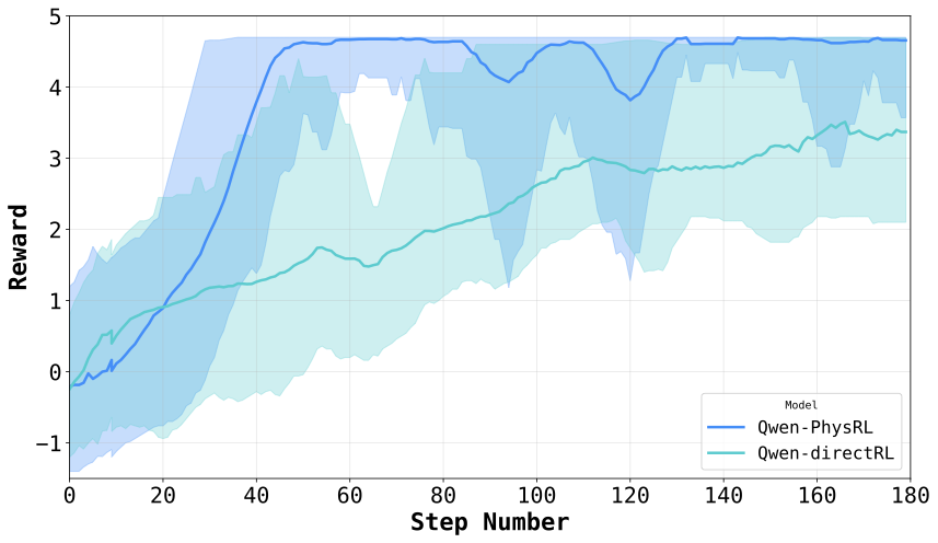
GRPO Convergence and Stability.
As shown in Figure 2, Qwen-PhysRL exhibits substantially faster convergence and higher final rewards than Qwen-DirectRL under identical GRPO training configurations, highlighting the importance of a physics-aware initialization for RL. Table 1 provides additional insight: the generic Qwen-Instruct backbone used in Qwen-DirectRL achieves higher rewards than the Qwen-Physics backbone used in Qwen-PhysRL during evaluation, indicating that general pretrained knowledge can partially compensate. However, despite this advantage, Qwen-Instruct fails to scale effectively under GRPO, exhibiting slower adaptation and early convergence to suboptimal policies. In contrast, the proposed two-stage approach consistently achieves superior performance across both Dynamic and Static settings.
Ablation Study
 style="width:90.0%" />
 style="width:100.0%" />
To examine the effect of our initial building-block fine-tuning on the spatial understanding of the target LLM $`\mathcal{F}`$, we analyze how attention is distributed across prompt tokens at different layers of the model by studying the attention score matrices produced during evaluation. We prompt the model with a fixed system prompt $`P`$, concatenated with a start–target map sequence $`M`$, to generate an answer sequence $`A`$, i.e., $`\mathcal{F}(P \!\cdot\! M) = A`$, where $`\cdot`$ denotes string concatenation. To obtain attention scores between prompt tokens and the newly generated output tokens, we concatenate the generated answer to the original prompt and perform a single forward pass over the full sequence, $`\mathcal{F}(P \!\cdot\! M \!\cdot\! A)`$. This pass yields the complete set of attention score matrices, including those corresponding to output tokens. For each decoder layer $`l \in \{1,\dots,L\}`$ and attention head $`h \in \{1,\dots,H\}`$, the model computes a raw attention score matrix as $`Q_{h,l} K_{h,l}^{\mathsf{T}}`$. We aggregate these matrices across heads by averaging to obtain a per-layer attention score matrix,
\text{AttScore}_l = \frac{1}{H} \sum_{h=1}^{H} Q_{h,l} K_{h,l}^{\mathsf{T}}.We then focus on the rows corresponding to the answer tokens, $`\text{AttScore}_l[|P \!\cdot\! M|:, :]`$, where each row represents the attention assigned to all prompt tokens during the generation of a specific output token. In the following, we summarize key observations derived from analyzing these attention patterns across layers.
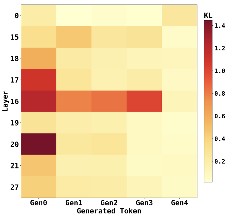
Observation 1.
Fine-tuning induces the most pronounced changes in attention distributions within the middle layers of the model, as confirmed by Figure 5. Among the 28 layers, layers 16 and 20 exhibit the highest KL divergence between Qwen-Physics and the generic Qwen-Instruct backbone, while the early (layer 0) and final (layer 27) layers show substantially smaller deviations. This indicates that the adaptation introduced by fine-tuning is concentrated in intermediate layers rather than being uniformly distributed across the network.
Observation 2.
Qwen-Physics assigns closer attention to
spatially informative ASCII tokens, such as # and *, compared to
Qwen-Instruct. As shown in
Figure 4, the increased attention to these
tokens is most prominent in the same middle layers identified in
Observation 1. This suggests that the layers undergoing the largest
adaptation are also those most responsible for encoding spatial
structure, enabling the model to better focus on salient regions of the
map $`M`$ during spatial reasoning.
Observation 3.
Across most layers, Qwen-Physics consistently allocates more attention to the system prompt $`P`$ than to the map region, except in the earliest layers. Notably, the system prompt contains approximately $`1.8\times`$ more tokens than the map region $`M`$, yet Figure 6 shows an attention gap that is substantially larger than what token count alone would suggest. This gap narrows in the middle layers, which, as shown in Observations 1 and 2, are more actively involved in spatial reasoning. This behavior is consistent with prior findings that textual context can dominate attention allocation in spatial reasoning and vision–language models . The earliest layers, such as layer 0, allocate attention more evenly across different parts of the input, reflecting a coarse, global skimming behavior, as illustrated in both Figure 6 and Figure 4.
Conclusion
This paper presents a two-stage training pipeline that enables spatial understanding, reasoning, and planning capabilities in large language models. Our approach first builds a foundation of atomic spatial relations through supervised fine-tuning and then augments it with multi-step planning ability using a closed-loop GRPO-based reinforcement learning stage. This combination equips the model with both task-relevant physical knowledge and a learned policy that effectively composes these primitives to solve more complex spatial planning problems, without relying solely on reinforcement learning to discover representations and planning strategies simultaneously. Experimental results demonstrate that models trained under this framework exhibit a newfound understanding of spatial properties and planning, substantially outperforming generic LLM baselines on challenging spatial planning tasks. Moreover, compared to end-to-end reinforcement learning applied to an unadapted backbone model, our pipeline converges faster and exhibits more stable training under identical settings. Through ablation studies and attention analysis, we further identify the decoder layers most affected by training and show that our approach systematically shifts attention toward task-critical tokens, providing evidence of more structured internal reasoning. While our evaluation focuses on a specific class of spatial planning problems, we believe that the underlying principle of learning reusable building blocks and composing them through reinforcement learning is broadly applicable. We view this work as a step toward more modular and interpretable approaches for teaching complex reasoning skills to language models, and we leave the exploration of additional tasks and modalities to future work.
Environment Setup Example
You are an expert at analyzing ASCII art shapes. Two shapes are provided:
Shape A (the target) and Shape B (the current state), separated by '%$%$%$%'.
Each line of the shapes starts and ends with a star (*) character.

Your goal is to transform Shape B into Shape A
by analyzing one type of transformation at a time.

You may analyze rotation, translation, or scaling --- but try to analyze
DIFFERENT types rather than repeating.

You have already analyzed: {analyzed}

IMPORTANT: Choose a transformation type you haven't analyzed yet if possible.

TASK 1 - ROTATION:
If analyzing rotation: Determine what rotation is needed to transform Shape B
into Shape A.
Classify using exactly one of these labels:
  - 'no_rotation': The shapes have the same orientation (0 rotation needed)
  - 'quarter_rotation': Shape B needs a 90 degrees rotation to match Shape A
  - 'slight_rotation': Shape B needs a small rotation (<90 degrees)
  to match Shape A

TASK 2 - TRANSLATION:
If analyzing translation: Determine how Shape B must be moved to match Shape
A's position.
Classify using exactly one of these labels:
  - 'no_translation': Shapes are already in the same position
  - 'up': Shape B must be moved up to match Shape A
  - 'down': Shape B must be moved down to match Shape A
  - 'left': Shape B must be moved left to match Shape A
  - 'right': Shape B must be moved right to match Shape A

TASK 3 - SCALING:
If analyzing scaling: Determine the size adjustment needed to transform Shape B
to match Shape A.
Classify using exactly one of these labels:
  - 'no_scaling': Both shapes have the same size
  - 'double_size': Shape B is half size and must be enlarged to match Shape A
  - 'half_size': Shape B is twice as large and must be shrunk to match Shape A

INSTRUCTIONS:
1. Identify which transformation type would be most useful to analyze now
2. Carefully compare both ASCII art shapes
3. Determine the transformation needed to convert Shape B into Shape A
4. Respond with the appropriate label inside <answer></answer> tags You are an expert at analyzing ASCII art shapes. Two shapes are provided:
Shape A (the target) and Shape B (the current state), separated by '%$%$%$%'.
Each line of the shapes starts and ends with a star (*) character.
Your goal is to transform Shape B into Shape A
by analyzing one type of transformation at a time.
You may analyze rotation, translation, or scaling --- but try to analyze
DIFFERENT types rather than repeating.
CRITICAL INSTRUCTION: THE MAP IS NOT UPDATING
The Shape B shown below is the **STATIC INITIAL STATE**
It does **NOT** reflect the moves you have already made.
You must RELY ON YOUR MEMORY of the following actions you have already performed:
HISTORY OF ACTIONS: [{analyzed}]
To solve this:
1. Look at the Initial Shape B.
2. Mentally apply the 'HISTORY OF ACTIONS' to it to imagine the *current* state.
3. Determine the NEXT step needed from that imagined state.
4. Choose a transformation type you haven't analyzed yet if possible.
TASK 1 - ROTATION:
If analyzing rotation: Determine what rotation is needed to transform Shape B
into Shape A.
Classify using exactly one of these labels:
- 'no_rotation': The shapes have the same orientation (0 rotation needed)
- 'quarter_rotation': Shape B needs a 90 degrees rotation to match Shape A
- 'slight_rotation': Shape B needs a small rotation (<90 degrees)
to match Shape A
TASK 2 - TRANSLATION:
If analyzing translation: Determine how Shape B must be moved to match Shape
A's position.
Classify using exactly one of these labels:
- 'no_translation': Shapes are already in the same position
- 'up': Shape B must be moved up to match Shape A
- 'down': Shape B must be moved down to match Shape A
- 'left': Shape B must be moved left to match Shape A
- 'right': Shape B must be moved right to match Shape A
TASK 3 - SCALING:
If analyzing scaling: Determine the size adjustment needed to transform Shape B
to match Shape A.
Classify using exactly one of these labels:
- 'no_scaling': Both shapes have the same size
- 'double_size': Shape B is half size and must be enlarged to match Shape A
- 'half_size': Shape B is twice as large and must be shrunk to match Shape A
INSTRUCTIONS:
1. Identify which transformation type would be most useful to analyze now
2. Carefully compare both ASCII art shapes
3. Determine the transformation needed to convert Shape B into Shape A
4. Respond with the appropriate label inside <answer></answer> tags
TARGET (Shape A):
*                           *
*                           *
*                           *
*                           *
*                           *
*                           *
*                           *
*                           *
*                           *
*                           *
*                           *
*                           *
*                           *
*                           *
*                           *
*                           *
*                           *
*                           *
*                           *
*                        ## *
*                      ##  #*
*                    ##     *
*                  ##     ##*
*                ##     ##  *
*                 ##  ##    *
*                   ##      *
*                           *
%$%$%$%
CURRENT (Shape B):
*                           *
*                           *
*            #              *
*          ## ##            *
*           #   #           *
*            ## ##          *
*              #            *
*                           *
*                           *
*                           *
*                           *
*                           *
*                           *
*                           *
*                           *
*                           *
*                           *
*                           *
*                           *
*                           *
*                           *
*                           *
*                           *
*                           *
*                           *
*                           *
*                           *
------------------------------
$`\star`$ Ground-Truth: double size, quarter rotation, right, down, down.
$`\times`$ Qwen-Instruct: slight rotation, slight rotation, slight rotation, slight rotation, slight rotation.
$`\times`$ Qwen-Physics: slight rotation, quarter rotation, slight rotation, slight rotation, slight rotation.
$`\times`$ Qwen-DirectRL: double size, quarter rotation, down, down, up.
$`\checkmark`$ Qwen-PhysRL (ours): double size, quarter rotation, right, down, down.
Random Policy Reward Calculation
To establish a baseline for the random policy $`\pi_{\text{rnd}}`$, we analytically derive the expected reward $`E[R_k]`$ at step $`k`$. An action $`a`$ yields a positive reward only if its usage count $`N_a`$ over the preceding $`k\!-\!1`$ steps does not exceed its ground-truth quota $`C_a`$. We model $`N_a`$ as a binomial random variable, $`N_a \sim \mathrm{Binomial}(k-1, 1/|\mathcal{A}|)`$, reflecting uniform random action selection. The expected reward at step $`k`$ is therefore given by
\begin{equation}
E[R_k] = \sum_{a \in GT} r(a)\,\mathbb{P}(N_a < C_a)
\;-\;
\lambda \!\left( 1 - \sum_{a \in GT} \mathbb{P}(N_a < C_a) \right),
\end{equation}where $`GT`$ denotes the set of ground-truth required actions, $`r(a)`$ is the reward associated with a valid action, and $`\lambda`$ is the penalty incurred for an invalid action. The probability term expands as the cumulative binomial sum
\begin{equation}
\mathbb{P}(N_a < C_a) = \sum_{i=0}^{C_a-1} \binom{k-1}{i}
\left(\frac{1}{|\mathcal{A}|}\right)^i
\left(1-\frac{1}{|\mathcal{A}|}\right)^{k-1-i}.
\end{equation}For the subset of samples considered in our evaluation, the ground-truth action quotas consist of two occurrences of one translation direction ($`C=2`$), one occurrence of another translation direction ($`C=1`$), and a single occurrence each for rotation and scaling ($`C=1`$). The expected cumulative reward up to step $`K`$ then follows directly as $`\sum_{j=1}^{K} E[R_j]`$.
📊 논문 시각자료 (Figures)