MSACL Multi-Step Actor-Critic Learning with Lyapunov Certificates for Exponentially Stabilizing Control
📝 Original Paper Info
- Title: MSACL Multi-Step Actor-Critic Learning with Lyapunov Certificates for Exponentially Stabilizing Control- ArXiv ID: 2512.24955
- Date: 2025-12-31
- Authors: Yongwei Zhang, Yuanzhe Xing, Quan Quan, Zhikun She
📝 Abstract
Achieving provable stability in model-free reinforcement learning (RL) remains a challenge, particularly in balancing exploration with rigorous safety. This article introduces MSACL, a framework that integrates exponential stability theory with maximum entropy RL through multi-step Lyapunov certificate learning. Unlike methods relying on complex reward engineering, MSACL utilizes off-policy multi-step data to learn Lyapunov certificates satisfying theoretical stability conditions. By introducing Exponential Stability Labels (ESL) and a $λ$-weighted aggregation mechanism, the framework effectively balances the bias-variance trade-off in multi-step learning. Policy optimization is guided by a stability-aware advantage function, ensuring the learned policy promotes rapid Lyapunov descent. We evaluate MSACL across six benchmarks, including stabilization and nonlinear tracking tasks, demonstrating its superiority over state-of-the-art Lyapunov-based RL algorithms. MSACL achieves exponential stability and rapid convergence under simple rewards, while exhibiting significant robustness to uncertainties and generalization to unseen trajectories. Sensitivity analysis establishes the multi-step horizon $n=20$ as a robust default across diverse systems. By linking Lyapunov theory with off-policy actor-critic frameworks, MSACL provides a foundation for verifiably safe learning-based control. Source code and benchmark environments will be made publicly available.💡 Summary & Analysis
1. **Exponential Stability Guarantee via Multi-Step Learning:** The MSACL framework integrates exponential stability conditions into Lyapunov certificate learning, ensuring the system converges to equilibrium exponentially. 2. **Sample-Efficient Off-Policy Framework:** Our framework, developed within the maximum entropy RL paradigm, enables efficient off-policy learning by correcting for distribution shifts with trajectory-wise importance sampling. 3. **Comprehensive Benchmarking System:** We created a suite of six nonlinear dynamical environments to rigorously evaluate and standardize Lyapunov-based RL algorithms.📄 Full Paper Content (ArXiv Source)
Model-free control, Exponential stability, Lyapunov certificates, Multi-step data collection and utilization, Off-policy RL, Maximum entropy RL.
Introduction
learning (RL) has emerged as a powerful paradigm for controlling complex, nonlinear dynamical systems without requiring analytical models . Despite its empirical success in high-dimensional tasks , the widespread deployment of RL in safety-critical applications, including autonomous driving and human-robot interaction, remains constrained by the lack of formal reliability guarantees . In these domains, stability is not merely a desirable metric but an imperative constraint; failure to maintain the system within a safe operating region can lead to catastrophic consequences. While approaches like constrained Markov Decision Processes (cMDPs) and Hamilton-Jacobi reachability analysis offer partial solutions, certificate-based methods have established themselves as the gold standard for verifying learning agents. By leveraging rigorous control-theoretic tools, specifically Lyapunov functions for asymptotic stability and control barrier functions (CBFs) for set invariance , these methods provide concise, data-driven proofs that guarantee the system will converge to an equilibrium or remain strictly within safety boundaries, offering a level of assurance that standard reward-driven learning cannot match.
The synthesis of stability and safety certificates has undergone a paradigm shift from computationally expensive analytical methods, such as sum-of-squares (SOS) optimization with its inherent restriction to polynomial dynamics , to scalable neural approaches. Around 2018, foundational work on neural certificates emerged, marking a turning point in bridging black-box learning with verifiable control. Early efforts by Berkenkamp et al. employed Gaussian Processes (GP) to learn Lyapunov functions for safe exploration, while Richards et al. and Chow et al. developed theoretical frameworks for synthesizing Lyapunov functions to estimate regions of attraction. These studies established that Lyapunov certificates as well as barrier-based counterparts provide a rigorous mathematical foundation for analyzing the stability and safety of nonlinear systems. Building on this verification-centric perspective, recent research has advanced toward the joint synthesis of policies and certificates: Chang et al. , for instance, showed that a neural certificate can act as a “critic” or supervision signal during training, directly guiding policy learning to satisfy formal stability conditions. This evolution underscores the dual role of learned certificates, which not only enable post-hoc safety verification but also actively shape the learning process to ensure stability and safety by design, offering guarantees that standard trial-and-error reinforcement learning cannot provide.
To enable effective learning in complex continuous spaces, we build our approach upon the framework of Maximum Entropy Reinforcement Learning (MERL). Algorithms such as Soft Actor-Critic (SAC) and its distributional variants like DSAC maximize not just the expected return but also the entropy of the policy. This entropy regularization encourages robust exploration and prevents the policy from converging prematurely to suboptimal deterministic behaviors. Given its superior sample efficiency and robustness to disturbances, the maximum entropy framework serves as an ideal substrate for developing advanced, stability-aware control algorithms.
However, standard model-free RL algorithms, including DDPG , TRPO , PPO , TD3 , D4PG , SAC, and DSAC, face significant limitations when applied to stabilization or tracking tasks. First, they lack intrinsic stability guarantees; since policies trained via these methods optimize solely for scalar reward maximization, stability is essentially an incidental byproduct that is achieved only when the agent implicitly discovers stable behaviors during the exploration process, rather than being structurally enforced. Second, the efficacy of these algorithms relies heavily on exhaustive reward engineering, requiring practitioners to laboriously calibrate coefficients for state deviation, control effort, and auxiliary terms to elicit stable behavior. Our proposed framework, MSACL (Multi-Step Actor-Critic Learning with Lyapunov Certificates), directly addresses these shortcomings. By adopting a formulation rooted in quadratic performance functionals such as LQR-like costs, MSACL eliminates the need for heuristic reward shaping. Most importantly, it guarantees stability by design, ensuring that the synthesized controller is not only high-performing but also mathematically certifiable.
While Lyapunov-based RL algorithms have been proposed to mitigate the two issues above, existing methods exhibit distinct shortcomings. The Policy Optimization with Lyapunov Certificates (POLYC) algorithm offers theoretical guarantees but relies on on-policy learning, which results in prohibitive sample complexity for physical systems. Conversely, the Lyapunov-based Actor-Critic (LAC) algorithm introduces an off-policy approach but fundamentally misaligns the objective: it minimizes a stability risk rather than a comprehensive control cost. This often leads to aggressive controllers that stabilize the system at the cost of excessive control effort, rendering them impractical for real-world actuators. Moreover, POLYC and LAC typically certify only asymptotic stability, a relatively weaker stability notion that ensures convergence but lacks the guaranteed exponential rate of decay. In practice, this guarantees eventual convergence but fails to impose a minimum convergence rate, often resulting in sluggish transient responses unacceptable for high-performance tasks. To overcome these limitations, MSACL is built upon an off-policy framework , significantly improving data efficiency by leveraging historical agent-environment interaction data. Unlike LAC, MSACL optimizes a comprehensive objective covering both state regulation and control effort while enforcing exponential stability, which guarantees faster convergence rates and rigorous stability margins.
Another critical innovation of our approach is the utilization of multi-step data. Existing RL and Lyapunov-based methods typically rely on single-step transitions to enforce learning constraints. This pointwise reliance is susceptible to significant discretization errors when approximating the continuous-time Lie derivative of the Lyapunov function, particularly in the presence of local noise. To mitigate this and capture long-horizon dynamics, we introduce a multi-step learning mechanism. By training on $`n`$-step trajectories, we effectively bridge the gap between temporal difference learning and rigorous stability verification. We integrate this multi-step data with exponential stability theory to form a robust constraint mechanism. This allows the agent to learn a Lyapunov function that certifies exponential convergence over trajectory segments, rather than just instantaneous descent, thereby reconciling rigorous stability requirements with the need for flexible exploration.
In summary, this article presents a comprehensive RL framework for model-free exponentially stabilizing control. The main contributions are summarized as follows:
-
Exponential Stability Guarantee via Multi-Step Learning: We introduce the MSACL framework, which integrates exponential stability conditions into Lyapunov certificate learning using a multi-step data utilization mechanism. By employing Exponential Stability Labels (ESL), our approach enforces that the system state converges to the equilibrium exponentially, providing stronger performance guarantees than conventional asymptotic convergence methods.
-
Sample-Efficient Off-Policy Framework: Developed within the maximum entropy RL paradigm, our framework enables efficient off-policy learning. By incorporating trajectory-wise importance sampling to correct for distribution shifts, MSACL allows for effective reuse of historical interaction data, significantly reducing sample complexity compared to existing on-policy Lyapunov-based RL algorithms.
-
Comprehensive Benchmarking System: We developed a diverse suite of six nonlinear dynamical environments, spanning four stabilization tasks (e.g., VanderPol) and two high-dimensional tracking tasks (e.g., Quadrotor Trajectory Tracking), to rigorously evaluate and provide a standard for Lyapunov-based RL algorithms.
-
Robustness and Generalization Verification: Our methodology demonstrates significant resilience to stochastic process noise and parametric uncertainties. Furthermore, in tracking scenarios, the learned neural policies exhibit robust generalization capabilities, maintaining high-precision performance even when navigating geometrically distinct, unseen reference trajectories.
-
Bias-Variance Trade-off Analysis: We provide a systematic analysis of the multi-step horizon parameter $`n`$ and its impact on stability learning. Through the introduction of $`\lambda`$-weighted aggregation, we effectively manage the trade-off between estimation bias (associated with small $`n`$) and sampling variance (associated with large $`n`$), establishing as a robust heuristic for diverse control applications.
The remainder of this article is organized as follows. Section 2 formulates the stabilization and tracking problems and establishes the theoretical foundations, including the criteria for exponential stability and the maximum entropy reinforcement learning framework. Section 3 details the methodology for learning the Lyapunov certificate, specifically describing the multi-step data collection strategy and the loss functions designed to enforce formal stability conditions. Section 4 presents the learning process for the neural control policy, deriving the optimization objectives for the soft Q-networks, the policy network, and the temperature coefficient. Section 5 reports the experimental results, providing a comprehensive comparison with baseline algorithms across six benchmark environments, followed by an evaluation of robustness, generalization capabilities, and parameter sensitivity. Finally, Section 6 provides a discussion on the underlying design philosophy and concludes the article.
Preliminaries
In this section, we establish the theoretical foundations for the proposed MSACL framework. We first define the stabilization and tracking problems for unknown discrete-time systems. Subsequently, the concept of exponential stability is introduced along with a Lyapunov-based certificate lemma, providing the criteria for convergence guarantees. Finally, we present the maximum entropy reinforcement learning framework, bridging Lyapunov-based control with model-free actor-critic optimization.
Problem Statement
In this article, we study the stabilization and tracking problems for general discrete-time deterministic control systems:
\begin{equation}
\label{control_system}
    \mathbf{x}_{t+1} = f(\mathbf{x}_t, \mathbf{u}_t),
\end{equation}where $`\mathbf{x}_t \in \mathcal{X} \subseteq \mathbb{R}^n`$ denotes the state at time $`t`$, $`\mathbf{u}_t \in \mathcal{U} \subseteq \mathbb{R}^m`$ represents the control input, $`\mathcal{X}`$ and $`\mathcal{U}`$ denote the sets of admissible states and control inputs, respectively, and $`f: \mathcal{X} \times \mathcal{U} \to \mathcal{X}`$ is the flow map. We assume that $`f`$ is unknown in our setting, thus focusing on model-free control. It is worth noting that the discrete-time framework presented in this article can be similarly extended to the continuous-time case; interested readers may refer to and for further details.
In the context of control systems, our objective is to find a state feedback policy $`\pi: \mathcal{X} \to \mathcal{U}`$ such that the control input $`\mathbf{u}_t = \pi(\mathbf{x}_t)`$ renders the closed-loop system $`\mathbf{x}_{t+1} = f(\mathbf{x}_t, \pi(\mathbf{x}_t))`$ to satisfy desired properties (e.g., stability, safety). For clarity, we consider the scenario where the state $`\mathbf{x}_t`$ is fully observable, and the policy $`\pi`$ is a time-invariant mapping. Specifically, we focus on tasks including
-
Stabilization: The objective is to find a policy $`\pi`$ such that the state ultimately converges to a target state $`\mathbf{x}_g \in \mathcal{X}`$. Without loss of generality, we assume $`\mathbf{x}_g`$ to be the origin, i.e., $`\mathbf{x}_g = \mathbf{0}`$.
-
Tracking: The goal is to find a policy $`\pi`$ such that the state $`\mathbf{x}_t`$ eventually converges to a reference signal $`\mathbf{x}_t^{\text{ref}}`$ (which may represent a desired trajectory, velocity, or attitude). We define the tracking error as $`\mathbf{e}_t = \mathbf{x}_t - \mathbf{x}_t^{\text{ref}}`$, thereby transforming the tracking task into a stabilization task where $`\mathbf{e}_t`$ must converge to zero.
In brief, the core problem addressed in this article is formulated as follows:
Problem 1. For the control system ([control_system]), find a policy $`\pi`$ such that: (i) in stabilization tasks, $`\mathbf{x}_t \to \mathbf{0}`$; (ii) in tracking tasks, $`\mathbf{e}_t \to \mathbf{0}`$. Moreover, the policy should be optimized to achieve the fastest possible convergence rate (e.g., exponential stability).
Exponential Stability and Lyapunov Certificates
Definition 1. *For the control system ([control_system]), the equilibrium point $`\mathbf{x}_g = \mathbf{0}`$ is said to be exponentially stable if there exist constants $`C > 0`$ and $`0 < \eta < 1`$ such that
\begin{equation}
\|\mathbf{x}_t - \mathbf{x}_g\| \leq C \eta^t \|\mathbf{x}_0 - \mathbf{x}_g\|, \quad \forall \mathbf{x}_0 \in \mathcal{X}_0,
\end{equation}where $`\mathbf{x}_0 \in \mathcal{X}_0 \subseteq \mathcal{X}`$ denotes the initial state and $`t \in \mathbb{Z}_{\geq 0}`$.*
To guarantee that a closed-loop system is exponentially stable with respect to $`\mathbf{x}_g`$, we introduce the following lemma:
Lemma 1. *For the control system ([control_system]), if there exists a continuous function $`V: \mathcal{X} \mapsto \mathbb{R}`$ and positive constants $`\alpha_1, \alpha_2 > 0`$ and $`0 < \alpha_3 < 1`$ satisfying:
\begin{equation}
\label{thm_con}
    \begin{aligned}
    \alpha_1 \|\mathbf{x}_t\|^2 \leq V(\mathbf{x}_t) &\leq \alpha_2 \|\mathbf{x}_t\|^2, \\
    V(\mathbf{x}_{t+1}) - V(\mathbf{x}_t) &\leq -\alpha_3 V(\mathbf{x}_t),
    \end{aligned}
\end{equation}for all $`t \in \mathbb{Z}_{\geq 0}`$, where $`\mathbf{x}_{t+1} = f(\mathbf{x}_t, \mathbf{u}_t)`$, then the origin $`\mathbf{x}_g = \mathbf{0}`$ is exponentially stable. The function $`V`$ is referred to as an exponentially stabilizing control Lyapunov function (ESCLF) .*
Proof: From the condition $`V(\mathbf{x}_{t+1}) \leq (1 - \alpha_3) V(\mathbf{x}_t)`$, we can iteratively derive the multi-step relationship:
\begin{equation}
\label{multi-step}
    \begin{aligned}
    V(\mathbf{x}_{t+1}) &\leq (1 - \alpha_3) V(\mathbf{x}_t), \\
    V(\mathbf{x}_{t+2}) &\leq (1 - \alpha_3) V(\mathbf{x}_{t+1}) \leq (1 - \alpha_3)^2 V(\mathbf{x}_t), \\
    &\vdots \\
    V(\mathbf{x}_{t+n}) &\leq (1 - \alpha_3) V(\mathbf{x}_{t+n-1}) \leq \dots \leq (1 - \alpha_3)^n V(\mathbf{x}_t).
    \end{aligned}
\end{equation}By incorporating the lower and upper quadratic bounds $`\alpha_1 \|\mathbf{x}_t\|^2 \leq V(\mathbf{x}_t) \leq \alpha_2 \|\mathbf{x}_t\|^2`$, it follows that:
\begin{equation}
\label{multi-step_conclusion}
    \|\mathbf{x}_{t+n}\| \leq \sqrt{\frac{\alpha_2}{\alpha_1}} (1 - \alpha_3)^{n/2} \|\mathbf{x}_t\|.
\end{equation}Specifically, by setting the initial time to $`t = 0`$ and denoting the current time step as $`n = t \in \mathbb{Z}_{\geq 0}`$, we obtain:
\begin{equation*}
    \|\mathbf{x}_t\| \leq \sqrt{\frac{\alpha_2}{\alpha_1}} (1 - \alpha_3)^{t/2} \|\mathbf{x}_0\|.
\end{equation*}Defining $`C = \sqrt{\alpha_2 / \alpha_1}`$ and $`\eta = \sqrt{1 - \alpha_3}`$, the result satisfies Definition 1, thereby proving that the control system ([control_system]) is exponentially stable with respect to $`\mathbf{x}_g = \mathbf{0}`$.
Standard RL and Maximum Entropy RL
In the reinforcement learning framework, the control system ([control_system]) is interpreted as a discrete-time deterministic environment, where $`\mathcal{X}`$ and $`\mathcal{U}`$ represent continuous state and action spaces, respectively. The application of control inputs to the system ([control_system]) corresponds to an agent interacting with this environment. Specifically, at each time step $`t`$, the agent observes the state $`\mathbf{x}_t`$ and executes an action $`\mathbf{u}_t`$ according to a policy $`\pi`$. Given a reward function $`r: \mathcal{X} \times \mathcal{U} \to \mathbb{R}`$, which is typically designed to penalize deviations from the target state $`\mathbf{x}_g`$ or reference $`\mathbf{x}_t^{\text{ref}}`$ in accordance with Problem 1, the environment returns a scalar reward $`r_t := r(\mathbf{x}_t, \mathbf{u}_t)`$ and transitions to the next state $`\mathbf{x}_{t+1}`$. Consequently, the interaction sequence is denoted by the transition tuple $`(\mathbf{x}_t, \mathbf{u}_t, r_t, \mathbf{x}_{t+1})`$.
While classical control often employs deterministic laws, this article utilizes stochastic policies to facilitate exploration and robustness within the maximum entropy RL (MERL) framework. A stochastic policy is defined as a mapping $`\pi: \mathcal{X} \to \mathcal{P}(\mathcal{U})`$, where $`\mathbf{u}_t \sim \pi(\cdot|\mathbf{x}_t)`$ is sampled from a probability distribution. We denote the state and state-action marginals induced by $`\pi`$ as $`\rho_\pi(\mathbf{x}_t)`$ and $`\rho_\pi(\mathbf{x}_t, \mathbf{u}_t)`$, respectively. Unlike standard RL, which maximizes the expected cumulative discounted reward, MERL optimizes an entropy-augmented objective:
\begin{equation}
\label{J_pi}
    J_{\pi} = \underset{(\mathbf{x}_{i \geq t}, \mathbf{u}_{i \geq t}) \sim \rho_{\pi}}{\mathbb{E}} \left[ \sum_{i=t}^{\infty} \gamma^{i-t} \left[ r_{i} + \alpha \mathcal{H}(\pi(\cdot|\mathbf{x}_{i})) \right] \right],
\end{equation}where $`\gamma \in [0, 1)`$ is the discount factor, $`\alpha > 0`$ is the temperature coefficient governing the trade-off between reward and exploration, and $`\mathcal{H}(\pi(\cdot|\mathbf{x})) = \mathbb{E}_{\mathbf{u} \sim \pi(\cdot|\mathbf{x})} [-\log \pi(\mathbf{u}|\mathbf{x})]`$ is the policy entropy.
The corresponding soft Q-function, $`Q^\pi(\mathbf{x}_t, \mathbf{u}_t)`$, represents the expected soft return, which comprises both rewards and entropy terms, starting from $`(\mathbf{x}_t, \mathbf{u}_t)`$ and following $`\pi`$ thereafter. The soft Bellman operator $`\mathcal{T}^\pi`$ is defined as:
\begin{equation}
\label{Bellman_operator}
    \begin{aligned}
        \mathcal{T}^{\pi}Q^{\pi}(\mathbf{x}_{t}, \mathbf{u}_{t}) \triangleq r_t + \gamma \underset{\mathbf{u}_{t+1} \sim \pi}{\mathbb{E}} \Big[ &Q^{\pi}(\mathbf{x}_{t+1}, \mathbf{u}_{t+1}) \\
        & - \alpha \log \pi(\mathbf{u}_{t+1}|\mathbf{x}_{t+1}) \Big],
    \end{aligned}
\end{equation}where $`\mathbf{x}_{t+1} = f(\mathbf{x}_t, \mathbf{u}_t)`$. In the soft policy iteration (SPI) algorithm , the policy is optimized by alternating between soft policy evaluation, where $`Q^\pi`$ is updated via iterative application of $`\mathcal{T}^\pi`$, and soft policy improvement, which is equivalent to finding a policy $`\pi`$ that maximizes the soft Q-function augmented with an entropy term for $`\mathbf{x}_t`$:
\begin{equation}
\label{max_softQ}
    \pi_{\rm new} = \arg\max_{\pi} \underset{\mathbf{x}_t \sim \rho_\pi, \mathbf{u}_t \sim \pi}{\mathbb{E}} \left[ Q^{\pi_{\rm old}}(\mathbf{x}_t, \mathbf{u}_t) - \alpha \log \pi(\mathbf{u}_t|\mathbf{x}_t) \right].
\end{equation}Although SPI converges to the optimal maximum entropy policy $`\pi^*`$ in tabular settings, practical control problems involve continuous spaces requiring function approximation. Thus, we parameterize the soft Q-function $`Q_\theta(\mathbf{x}_t, \mathbf{u}_t)`$ and the policy $`\pi_\phi(\mathbf{u}_t|\mathbf{x}_t)`$ using neural networks with parameters $`\theta`$ and $`\phi`$. We assume $`\pi_\phi`$ follows a diagonal Gaussian distribution with mean $`\mu_\phi(\mathbf{x}_t)`$ and standard deviation $`\sigma_\phi(\mathbf{x}_t)`$. Actions are sampled using the reparameterization trick: $`\mathbf{u}_t = g_\phi(\mathbf{x}_t; \epsilon_t)`$, where $`\epsilon_t \sim \mathcal{N}(\mathbf{0}, \mathbf{I}_m)`$, ensuring that the objective remains differentiable with respect to $`\phi`$.
Learning Lyapunov Certificate
In this section, we develop the learning mechanism for the Lyapunov certificate within a model-free framework. We first introduce a sliding-window data collection strategy to satisfy multi-step trajectory requirements. Subsequently, we design a comprehensive loss function for the Lyapunov network, incorporating boundedness constraints and a multi-step stability loss. To enhance training efficiency and robustness, we employ trajectory-wise importance sampling for off-policy correction, a labeling mechanism for positive and negative samples, and a $`\lambda`$-weighted aggregation to balance the bias-variance trade-off.
Data Collection
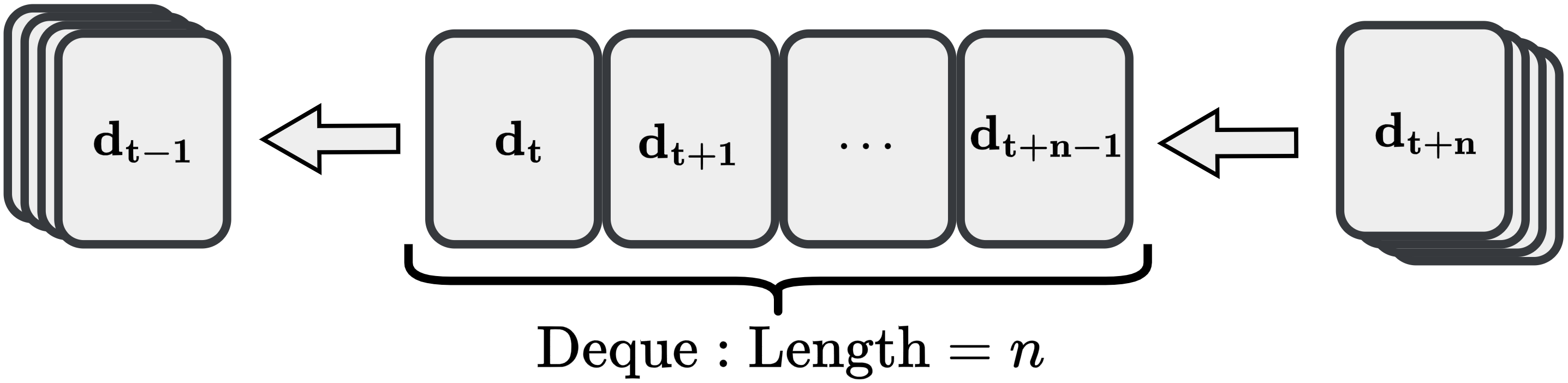
Our algorithm is developed within the maximum entropy RL framework, where data is acquired through agent-environment interactions with the system ([control_system]). Unlike the standard SAC algorithm that samples single-step transitions, we leverage the multi-step Lyapunov condition presented in ([multi-step]), which necessitates data sequences spanning $`n`$ consecutive steps. We define a single-step interaction tuple as $`\mathbf{d}_t = (\mathbf{x}_t, \mathbf{u}_t, r_t, \pi_\phi(\mathbf{u}_t|\mathbf{x}_t), \mathbf{x}_{t+1})`$, where $`\pi_\phi(\mathbf{u}_t|\mathbf{x}_t)`$ represents the probability density of sampling action $`\mathbf{u}_t`$ at state $`\mathbf{x}_t`$. The collected multi-step data consists of sequences $`\{\mathbf{d}_t, \mathbf{d}_{t+1}, \dots, \mathbf{d}_{t+n-1}\}`$, which are stored in the experience replay buffer $`\mathcal{D}`$.
Data storage commences only after $`n`$ consecutive steps have been accumulated. Specifically, during the initial $`n-1`$ steps of any rollout, no data is committed to $`\mathcal{D}`$. Once the rollout length reaches or exceeds $`n`$, the collection process begins. As illustrated in Fig. 1, we employ a double-ended queue (deque) to temporarily buffer interaction data. During each agent-environment interaction, new data enters the deque. Once the deque reaches a length of $`n`$, the complete $`n`$-step sequence is transferred to $`\mathcal{D}`$, and the oldest data point is removed to maintain the deque size, enabling a continuous sliding window for data collection.
Loss Function Design of Lyapunov Network
Similar to the soft Q-network and policy network, we introduce a Lyapunov network parameterized by $`\psi`$, denoted as $`V_\psi`$, to estimate the Lyapunov certificate. In designing the loss function for the Lyapunov certificate, we strictly adhere to the conditions established in Lemma 1, which encompass the boundedness and multi-step stability requirements.
(1) Boundedness Loss: Based on the first condition in Lemma 1, we construct the boundedness loss function to ensure the Lyapunov certificate is quadratically constrained:
\begin{equation}
\begin{aligned}
    \mathcal{L}_{\text{Bnd}}(\psi) = \frac{1}{Nn} & \sum_{i=1}^{N}\sum_{k=0}^{n-1} \Big[ \max\left( \alpha_1 \|\mathbf{x}_{t+k}^i\|^2 - V_\psi(\mathbf{x}_{t+k}^i), 0 \right) \\
    & + \max\left( V_\psi(\mathbf{x}_{t+k}^i) - \alpha_2 \|\mathbf{x}_{t+k}^i\|^2, 0 \right)\Big],
\end{aligned}
\end{equation}where $`N`$ denotes the number of multi-step trajectories in a batch, $`i`$ denotes the $`i`$-th multi-step sample in the batch, and $`n`$ represents the number of steps within each trajectory. This loss term explicitly constrains $`V_\psi`$ to satisfy the boundedness condition defined in ([thm_con]).
(2) Multi-step Stability Loss: Consider a sampled multi-step trajectory $`\{\mathbf{d}_t, \dots, \mathbf{d}_{t+n-1}\}`$ generated by a previous policy $`\pi_{\phi_{\text{old}}}`$. Since our goal is to train the Lyapunov certificate $`V_\psi`$ to be compatible with the current policy $`\pi_{\phi_{\text{new}}}`$ for subsequent policy updates, we must account for the off-policy nature of the data. We introduce trajectory-wise importance sampling to correct the distribution shift. For an $`n`$-step trajectory, the importance sampling ratio for the segment from $`t`$ to $`t+k`$ is defined as ($`k=1, 2, \dots, n-1`$):
\begin{equation}
\label{IS}
    \text{IS}_{\text{clip},k} = \prod_{j=t}^{t+k-1} \min \left( \frac{\pi_{\phi}(\mathbf{u}_j|\mathbf{x}_j)}{\pi_{\phi_{\text{old}}}(\mathbf{u}_j|\mathbf{x}_j)}, 1 \right).
\end{equation}Note that we apply a clipping operation to the importance sampling ratios to prevent variance explosion and enhance training stability.
Furthermore, we address the second condition in ([thm_con]), namely the stability requirement. While ([multi-step]) represents the ideal theoretical decay, empirical trajectories may not strictly satisfy the exponential stability bound in ([multi-step_conclusion]) during early stages of training. To bridge the gap between the stability condition and the stochastic samples, we introduce the concepts of positive and negative samples.
Definition 2. *Within an $`n`$-step sample, for a state $`\mathbf{x}_{t+k}`$, if it satisfies the exponential decay condition:
\begin{equation*}
        \|\mathbf{x}_{t+k}\| \leq \sqrt{\frac{\alpha_2}{\alpha_1}} (1 - \alpha_3)^{k/2} \|\mathbf{x}_t\|,
\end{equation*}then $`\mathbf{d}_{t+k}`$ is classified as a positive sample; otherwise, it is classified as a negative sample.*
Accordingly, we define the Exponential Stability Label (ESL) as:
\begin{equation*}
    \text{ESL}_{k} = \begin{cases}
    1, & \text{if } \|\mathbf{x}_{t+k}\| \leq \sqrt{\frac{\alpha_2}{\alpha_1}} (1 - \alpha_3)^{k/2} \|\mathbf{x}_t\| \\
    -1, & \text{otherwise}.
    \end{cases}
\end{equation*}This labeling mechanism allows the Lyapunov network to distinguish between transitions that contribute to system stability and those that violate the certificate requirements.
For trajectories composed of multi-step interaction data, we introduce a weighting factor $`\lambda \in (0, 1)`$, inspired by the (truncated) $`\lambda`$-return in reinforcement learning , to balance the trade-off between bias and variance. Specifically, in the stability condition $`V_\psi(\mathbf{x}_{t+k}) \leq (1-\alpha_3)^{k} V_\psi(\mathbf{x}_t)`$ from ([multi-step]), the parameter $`k`$ determines the temporal horizon of the system’s evolution. When $`k`$ is small, the short trajectory horizon provides a limited view of the system’s long-term dynamics under policy $`\pi_\phi`$. Given that the Lyapunov network is randomly initialized and potentially inaccurate in the early stages of training, relying on short-horizon data can introduce significant estimation bias.
Conversely, a larger $`k`$ captures more extensive information regarding the trajectory evolution (extended horizon), thereby providing a stronger and more accurate learning signal that reduces bias. However, since each transition is sampled from the environment, every step introduces stochasticity; consequently, longer trajectories accumulate higher cumulative variance. Therefore, a small $`k`$ leads to high bias but low variance, while a large $`k`$ results in low bias but high variance. To optimize this trade-off, we employ the weighting factor $`\lambda`$ to aggregate multi-step information.
By integrating the positive/negative sample labels with the weighting factor $`\lambda`$, we construct the Lyapunov stability loss to enforce a rigorous correspondence between empirical samples and the stability condition ([multi-step]):
\begin{equation}
\label{loss_diff_V}
    \mathcal{L}_{\text{Stab}}(\psi) = \frac{1}{N} \sum_{i=1}^N \left[ \sum_{k=1}^{n-1} \frac{\lambda^{k-1} \mathcal{L}_{\text{diff}, k}^{i}(\psi)}{\sum_{j=1}^{n-1} \lambda^{j-1}} \right],
\end{equation}and the step-wise difference loss $`\mathcal{L}_{\text{diff}, k}^{i}(\psi)`$ is defined as:
\begin{equation*}
\begin{aligned}
    \mathcal{L}_{\text{diff}, k}^{i}(\psi) = \,&\text{IS}_{\text{clip},k}^i \cdot \max\Big(0, \\
    &\text{ESL}_{k}^i \cdot \left(V_\psi(\mathbf{x}_{t+k}^i) - (1-\alpha_3)^{k} V_\psi(\mathbf{x}_t^i)\right)\Big).
\end{aligned}
\end{equation*}(3) Combined Lyapunov Loss: By integrating the boundedness and multi-step stability losses, the total loss function for optimizing the Lyapunov network is formulated as:
\begin{equation}
\label{loss_lya}
    \mathcal{L}_{\text{Lya}}(\psi) = \omega_{\text{Bnd}} \mathcal{L}_{\text{Bnd}}(\psi) + \omega_{\text{Stab}} \mathcal{L}_{\text{Stab}}(\psi),
\end{equation}where $`\omega_{\text{Bnd}}`$ and $`\omega_{\text{Stab}}`$ are positive weighting coefficients.
Learning Policy with Exponential Stability Constraints
This section presents the optimization framework for the proposed MSACL algorithm. We first establish the soft Q-network updates using multi-step Bellman residuals to enhance data efficiency. We then introduce a novel policy loss function that incorporates a stability advantage derived from the Lyapunov certificate, utilizing a PPO-style clipping mechanism to ensure robust convergence toward exponentially stable behavior. Finally, we describe the automated temperature adjustment and synthesize the complete actor-critic learning procedure.
Loss Function Design of Soft Q Networks
Based on the soft Bellman operator ([Bellman_operator]), we define the sampled Bellman residual for the $`i`$-th transition within a multi-step sequence for the soft Q-network $`Q_\theta`$ as:
\begin{equation}
\begin{aligned}
    \mathcal{B}_t^{i}(\theta) = Q_\theta(\mathbf{x}_t^i, \mathbf{u}_t^i) - \Big[ & r_t^i + \gamma Q_{\bar{\theta}}(\mathbf{x}_{t+1}^i, \mathbf{u}_{t+1}^i) \\
    & - \alpha \log \pi_{\phi}(\mathbf{u}_{t+1}^i|\mathbf{x}_{t+1}^i) \Big],
\end{aligned}
\end{equation}where $`Q_{\bar{\theta}}`$ denotes the target network parameterized by $`\bar{\theta}`$, which is updated via polyak averaging to stabilize the learning process. Utilizing the collected multi-step sequences, the loss function for the soft Q-network is defined as the mean squared Bellman error (MSBE) across the entire trajectory:
\begin{equation}
\label{loss_softQ}
    \mathcal{L}_{\text{SoftQ}}(\theta) = \frac{1}{Nn} \sum_{i=1}^{N} \sum_{k=0}^{n-1} (\mathcal{B}_{t+k}^{i}(\theta))^2.
\end{equation}While standard implementations of maximum entropy RL algorithms, such as SAC , typically set the upper limit of the inner summation in ([loss_softQ]) to zero (i.e., $`n=1`$) to utilize only single-step transitions, our formulation leverages the complete $`n`$-step sequence for parameter updates. Theoretically, minimizing the MSBE requires state-action pairs $`(\mathbf{x}_t, \mathbf{u}_t)`$ to be sampled from a distribution that ensures an unbiased stochastic gradient estimate. Specifically, the objective is given by:
\begin{equation*}
    \begin{aligned}
        \mathcal{J}_{\text{SoftQ}}(\theta)=&\underset{\mathbf{x}_t \sim \rho_\pi, \mathbf{u}_t \sim \pi}{\mathbb{E}}\Big[ Q_\theta(\mathbf{x}_t, \mathbf{u}_t) -  \Big( r_t + \gamma \underset{\mathbf{x}_{t+1} \sim \rho_\pi, \mathbf{u}_{t+1} \sim \pi}{\mathbb{E}}\\
        &\big(Q_{\bar{\theta}}(\mathbf{x}_{t+1}, \mathbf{u}_{t+1}) - \alpha \log \pi_{\phi}(\mathbf{u}_{t+1}|\mathbf{x}_{t+1})\big)  \Big) \Big]^2.
    \end{aligned}
\end{equation*}Strictly speaking, the transitions within a multi-step sequence are temporally correlated, and utilizing the full sequence simultaneously deviates from the independent and identically distributed (i.i.d.) sampling requirement commonly assumed in stochastic optimization. However, this approach represents a deliberate trade-off between mathematical rigor and sample efficiency. By incorporating all transitions within each collected sequence into the loss function, we significantly enhance the data utilization rate and the information density of each training batch. Experimental evidence suggests that as long as the sequence length $`n`$ remains moderate, the bias introduced by these short-term correlations does not undermine the stability of the Q-function learning. In practice, the benefits of improved sample efficiency and accelerated convergence often outweigh the theoretical concerns regarding strict uniform sampling, ultimately contributing to more robust control performance.
Remark 1. In the practical implementation of Algorithm [msacl], we utilize clipped double-Q learning with two networks, $`Q_{\theta_1}`$ and $`Q_{\theta_2}`$, to mitigate the overestimation bias of soft Q-values, as motivated by the TD3 framework . Furthermore, we incorporate the “delayed policy update” technique to ensure that the policy is updated against a more stable value function, thereby facilitating smoother convergence of the actor-critic process.
Loss Function Design of Policy Network
This subsection details the optimization process for the policy network, which integrates the maximum entropy objective with a Lyapunov-based stability constraint. In the standard SAC framework , policy optimization aims to maximize the expected soft Q-value. For the $`i`$-th multi-step sequence, the SAC-component of the loss function is expressed as:
\begin{equation*}
    \begin{aligned}
        \mathcal{L}_{\pi,\text{SAC}}^{i}(\phi) = \frac{1}{n} \sum_{k=0}^{n-1} \Big[ & Q_\theta(\mathbf{x}_{t+k}^i, g_\phi(\mathbf{x}_{t+k}^i;\epsilon_{t+k}^i)) \\
        & - \alpha \log \pi_\phi(g_\phi(\mathbf{x}_{t+k}^i;\epsilon_{t+k}^i) | \mathbf{x}_{t+k}^i) \Big].
    \end{aligned}
\end{equation*}To ensure the learned policy satisfies the exponential stability requirements, we utilize the learned Lyapunov certificate $`V_\psi`$ to guide the policy updates. Inspired by the Generalized Advantage Estimation (GAE) in PPO , we define a stability advantage function based on $`V_\psi`$, which serves as a metric for convergence performance:
\begin{equation}
    A_{t,k} = (1-\alpha_3)^k V_\psi(\mathbf{x}_t) - V_\psi(\mathbf{x}_{t+k}).
\end{equation}A positive stability advantage ($`A_{t,k} \geq 0`$) indicates that the system trajectory from $`\mathbf{x}_t`$ to $`\mathbf{x}_{t+k}`$ strictly adheres to the exponential decay condition. Maximizing this advantage encourages the policy to select actions that accelerate the decay of $`V_\psi`$, thereby directly increasing the state convergence rate toward the equilibrium $`\mathbf{x}_g`$. Conversely, $`A_{t,k} < 0`$ signifies a violation of the stability certificate, representing a disadvantage that the policy must learn to avoid. This stability-driven optimization paradigm aligns with recent developments in stable model-free control, such as D-learning . To robustly handle the bias-variance trade-off across varying horizons, we apply the weighting factor $`\lambda`$ to obtain the aggregated stability advantage:
\begin{equation}
    A_{t,\lambda} = \sum_{k=1}^{n-1} \frac{\lambda^{k-1} A_{t,k}}{\sum_{j=1}^{n-1} \lambda^{j-1}}.
\end{equation}For a multi-step sample $`\{\mathbf{d}_t, \dots, \mathbf{d}_{t+n-1}\}`$, we define the policy importance sampling ratio based on the initial transition as $`\rho^i(\phi) = \frac{\pi_\phi(\mathbf{u}_t^i|\mathbf{x}_t^i)}{\pi_{\phi_{\text{old}}}(\mathbf{u}_t^i|\mathbf{x}_t^i)}`$. Incorporating the clipping mechanism to prevent excessively large policy updates, the final policy loss function is formulated as:
\begin{equation}
\label{loss_policy}
\begin{aligned}
    \mathcal{L}_\pi(\phi) = -\frac{1}{N} \sum_{i=1}^N \Big[ & \mathcal{L}_{\pi,\text{SAC}}^{i}(\phi) + \min\Big(\rho^i(\phi) A_{t,\lambda}^i, \\
    & \text{clip}(\rho^i(\phi), 1-\varepsilon, 1+\varepsilon) A_{t,\lambda}^i \Big) \Big].
\end{aligned}
\end{equation}Remark 2. It is important to distinguish between the two importance sampling (IS) strategies employed in this article. In ([loss_diff_V]), sequence-level IS (from $`t`$ to $`t+k-1`$) is used to train the Lyapunov certificate $`V_\psi`$. While sequence-level IS typically introduces higher variance, it provides the low-bias correction necessary for the Lyapunov network to accurately reflect the stability of the current policy $`\pi_\phi`$ using off-policy data. Since the policy parameters are fixed during the Lyapunov update phase, this variance remains manageable via the truncation in ([IS]). However, when optimizing the policy $`\pi_\phi`$ itself, sequence-level IS would introduce prohibitive variance into the gradient estimates, often leading to training divergence. Consequently, following the design principle of PPO, we utilize only the first-step IS ratio $`\rho(\phi)`$ in ([loss_policy]). This approach effectively reduces the variance of the policy gradient, ensuring stable optimization while still benefiting from the multi-step stability information embedded within the weighted advantage $`A_{t,\lambda}`$.
Automated Temperature Adjustment
In maximum entropy RL, the temperature coefficient $`\alpha`$ in ([J_pi]) is critical for balancing exploration and exploitation. Following the automated entropy adjustment mechanism introduced in , we update $`\alpha`$ by minimizing the following loss function:
\begin{equation}
\label{loss_alpha}
    \mathcal{L}_{\text{Ent}}(\alpha) = \frac{1}{Nn} \sum_{i=1}^N \sum_{k=0}^{n-1} \left[ -\alpha \log \pi_\phi(\mathbf{u}_{t+k}^i|\mathbf{x}_{t+k}^i) - \alpha \bar{\mathcal{H}} \right],
\end{equation}where $`\bar{\mathcal{H}}`$ denotes the target entropy, typically set as $`\bar{\mathcal{H}} = -m`$, with $`m`$ representing the dimension of the action space.
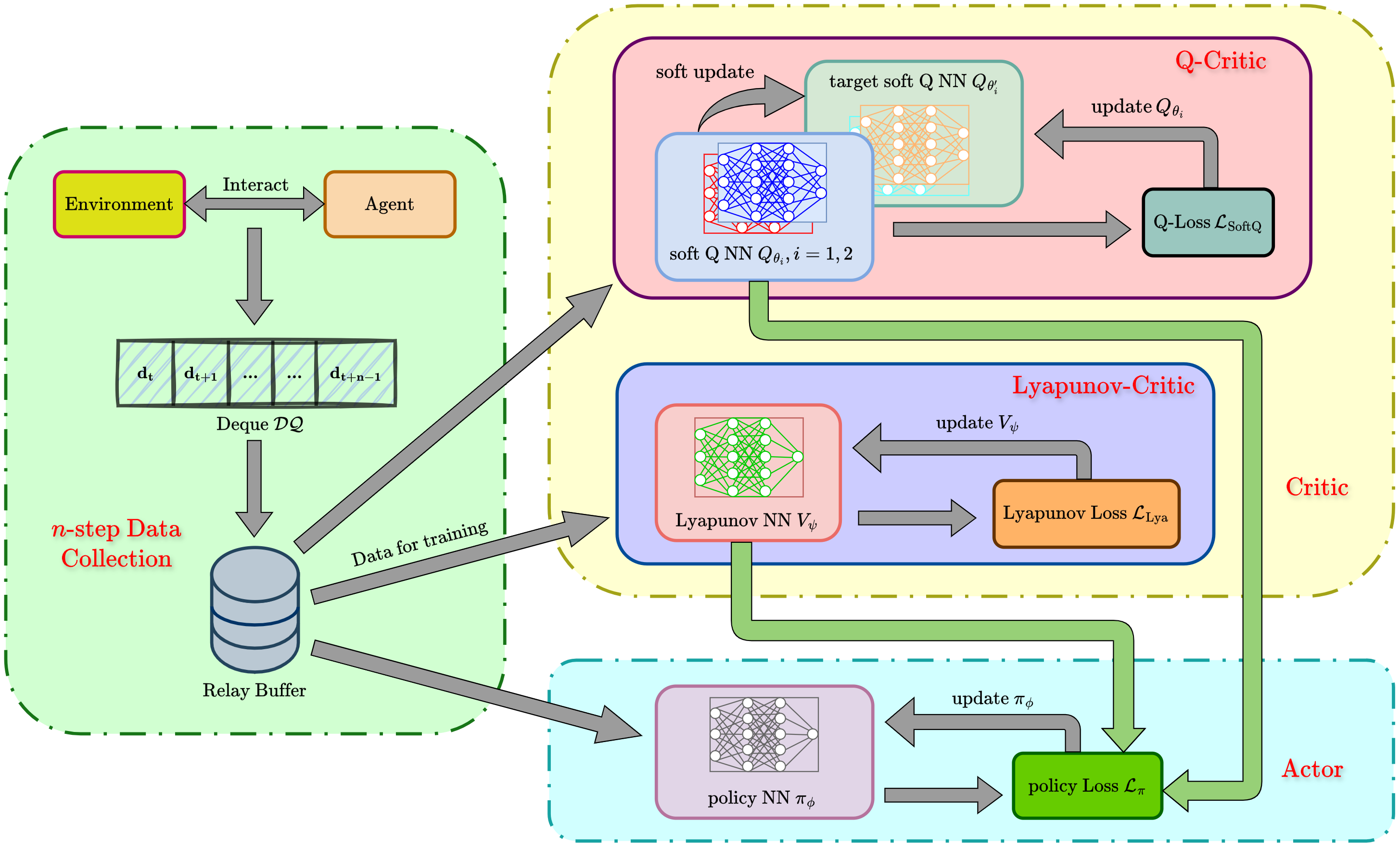
By integrating the loss functions for the soft Q-network $`Q_\theta`$, the Lyapunov network $`V_\psi`$, the policy network $`\pi_\phi`$, and the temperature coefficient $`\alpha`$, we iteratively update the parameters within an actor-critic framework using the Adam optimizer . The complete algorithmic procedure is summarized in Algorithm [msacl], and the overall flowchart is illustrated in Fig. 2.
Select action $`\mathbf{u}_t \sim \pi_{\phi}(\cdot|\mathbf{x}_t)`$ Obtain reward $`r_t`$ and observe next state $`\mathbf{x}_{t+1}`$ Store tuple $`\mathbf{d}_t = (\mathbf{x}_t, \mathbf{u}_t, r_t, \pi_{\phi}(\mathbf{u}_t|\mathbf{x}_t), \mathbf{x}_{t+1})`$ in $`\mathcal{DQ}`$ Store $`\{\mathbf{d}_i\}_{i=t}^{t+n-1} = \{\mathbf{d}_{t}, \dots, \mathbf{d}_{t+n-1}\}`$ in $`\mathcal{D}`$ Sample $`N`$ multi-step sequences $`\{\mathbf{d}_i\}_{i=t}^{t+n-1}`$ from $`\mathcal{D}`$ Update $`V_{\psi}`$ via $`\psi \leftarrow \psi - \beta_\psi \nabla_\psi \mathcal{L}_{\text{Lya}}(\psi)`$ Update $`Q_{\theta_i}`$ via $`\theta_i \leftarrow \theta_i - \beta_\theta \nabla_{\theta_i} \mathcal{L}_{\text{SoftQ}}(\theta_i)`$ Update $`\pi_\phi`$ via $`\phi \leftarrow \phi - \beta_\phi \nabla_\phi \mathcal{L}_{\pi}(\phi)`$ Update $`\alpha`$ via $`\alpha \leftarrow \alpha - \beta_\alpha \nabla_\alpha \mathcal{L}_{\text{Ent}}(\alpha)`$ Update target parameters: $`\bar{\theta}_i \leftarrow \tau \theta_i + (1-\tau) \bar{\theta}_i`$
Remark 3. In the flowchart of Algorithm
[msacl], we incorporate two implementation
refinements. Specifically, regarding footnote 1: for the soft Q-loss
function ([loss_softQ]), we replace the target
value $`Q_{\bar{\theta}}`$ with
$`\min\{Q_{\bar{\theta}_1}, Q_{\bar{\theta}_2}\}`$ to mitigate
overestimation bias, as noted in Remark
1. Regarding footnote 2: we implement
delayed updates for both the policy network $`\pi_\phi`$ and the
temperature coefficient $`\alpha`$. However, within each delayed update
cycle, we perform $`d`$ consecutive updates for these parameters as a
“delayed update compensation” mechanism to ensure adequate policy
improvement. These techniques are adapted from the cleanrl framework ,
and our experiments demonstrate that integrating these refinements
significantly enhances overall performance and training stability.
Experiments
In this section, we conduct a comprehensive experimental evaluation of the MSACL algorithm across six benchmark environments, encompassing both stabilization and high-dimensional nonlinear tracking tasks. We compare our approach against baseline model-free RL algorithms and Lyapunov-based RL algorithms using rigorous performance and stability metrics. The analysis further includes the visualization of learned Lyapunov certificates, extensive robustness and generalization testing under parametric uncertainties and stochastic noise, and a sensitivity study investigating the impact of the multi-step horizon $`n`$ on the learning process.
Benchmark Environments
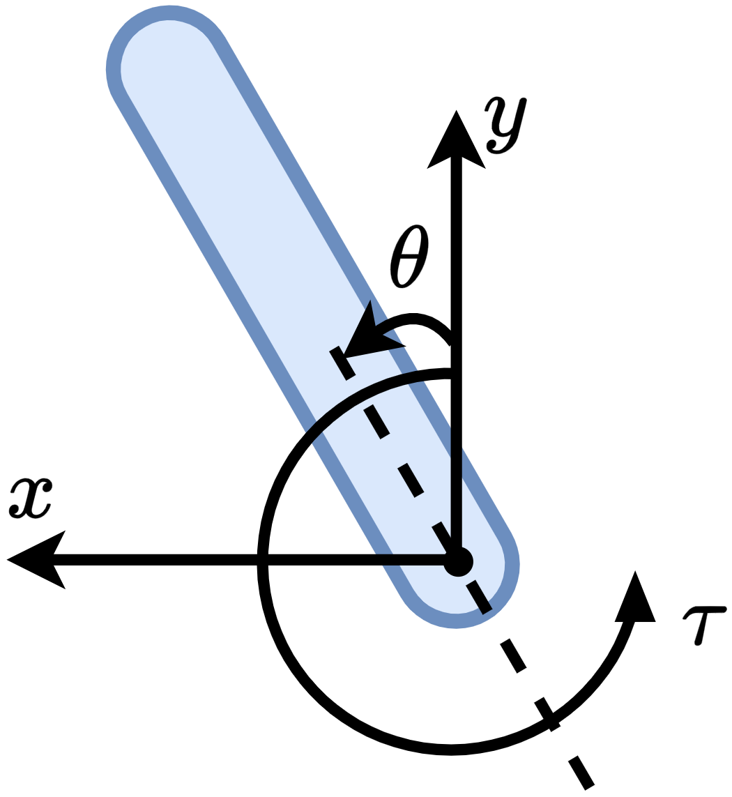
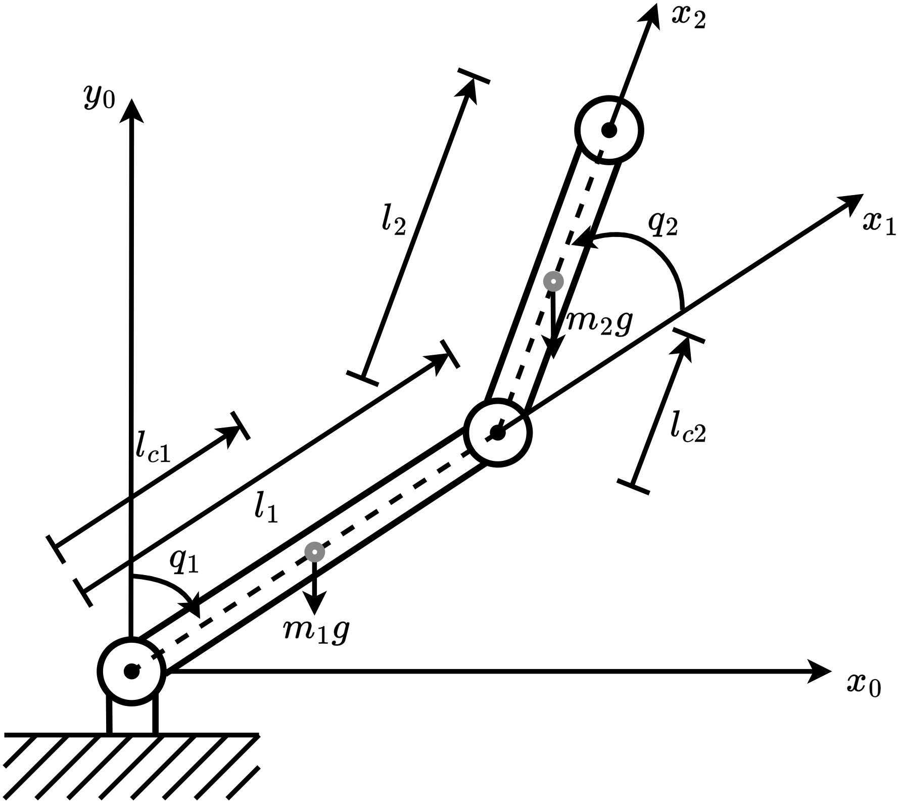
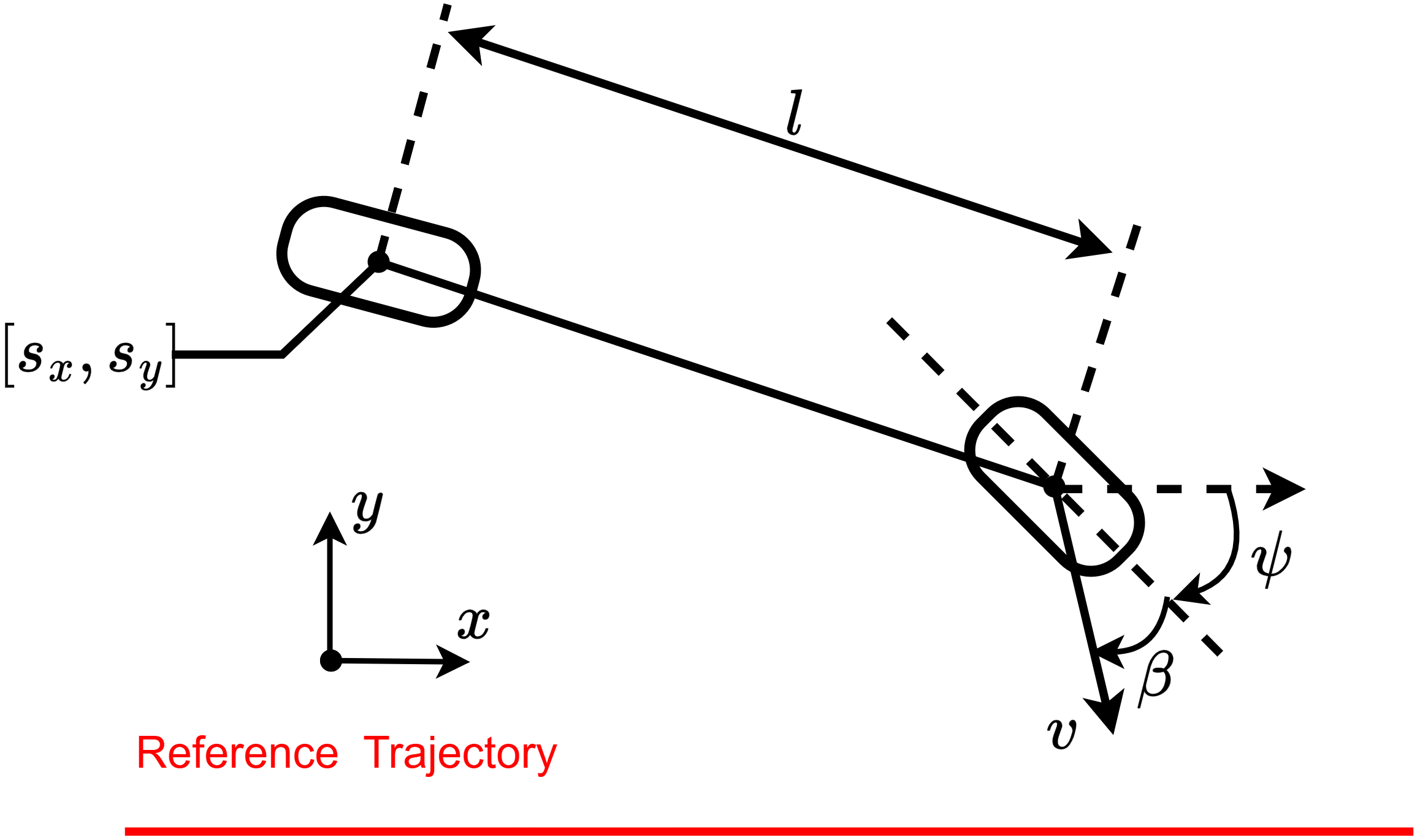
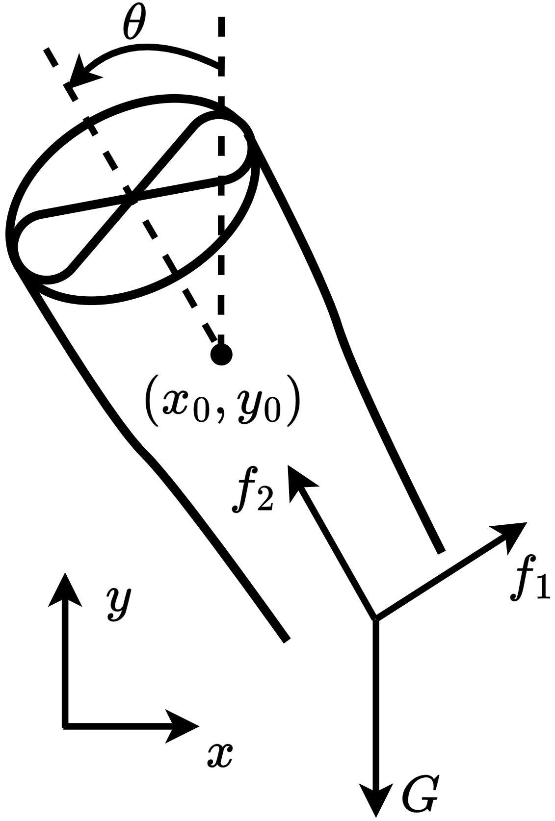
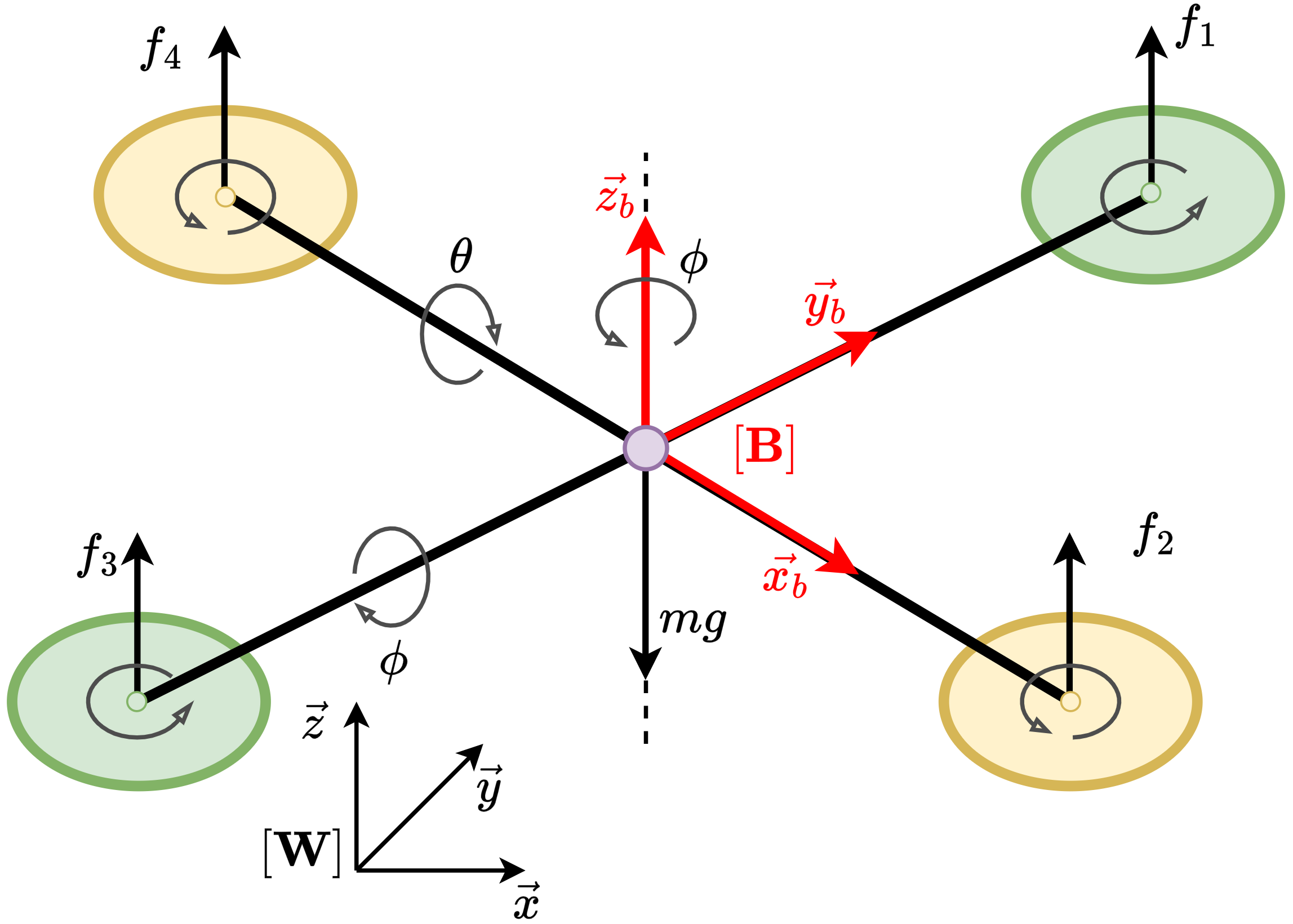
In this subsection, we present the benchmark environments utilized to evaluate the experimental performance of the proposed and baseline algorithms, encompassing both stabilization and tracking tasks. We categorize these environments by their primary control objectives. For stabilization tasks, the environments include: Controlled VanderPol (hereafter referred to as VanderPol), Pendulum, Planar DuctedFan (DuctedFan), and Two-link planar robot (Two-link). For tracking tasks, the benchmark comprises SingleCarTracking and QuadrotorTracking. As illustrated in Figure 3, comprehensive specifications and dynamical parameters for all environments are provided in Appendix [Appendix].
In stabilization tasks, the control objective is to drive the system state to the equilibrium point, i.e., $`\mathbf{x}_g = \mathbf{0} \in \mathbb{R}^n`$. In tracking tasks, the goal is to ensure the system state follows a time-varying reference trajectory $`\mathbf{x}_t^{\text{ref}}`$, which may represent desired coordinates, velocities, or attitudes. Across all tasks, we employ a unified reward structure:
\begin{equation}
\label{reward_function}
    r_t =
    \underbrace{-\left(\mathbf{x}_t^\top \mathbf{Q_r} \mathbf{x}_t + \mathbf{u}_t^\top \mathbf{R_r} \mathbf{u}_t\right)}_{\text{Penalty}}
    + \underbrace{r_{\mathrm{approach}}}_{\text{Encouragement}}
\end{equation}where the first term is a penalty term inspired by the performance functionals commonly utilized in optimal control , with $`\mathbf{Q_r}`$ and $`\mathbf{R_r}`$ being positive definite weight matrices. This term penalizes deviations from the equilibrium and excessive control effort at each time step, effectively minimizing the cumulative cost $`\sum_{t=0}^{\infty} \left[\mathbf{x}_t^\top \mathbf{Q_r} \mathbf{x}_t + \mathbf{u}_t^\top \mathbf{R_r} \mathbf{u}_t\right]`$. For tracking tasks, the state $`\mathbf{x}_t`$ in the penalty term is replaced by the tracking error $`\mathbf{e}_t = \mathbf{x}_t - \mathbf{x}_t^{\text{ref}}`$. The second term provides sparse encouragement, defined as:
\begin{equation*}
    r_{\mathrm{approach}} =
    \begin{cases}
    r_\delta, & \text{if } \|\mathbf{x}_t\|_\infty \leq \delta \\
    0,         & \text{otherwise}
    \end{cases}
\end{equation*}Specifically, when the state approaches the equilibrium (i.e., its infinity norm falls below a small threshold $`\delta`$, such as 0.01), the environment provides a constant positive reward $`r_\delta`$ (e.g., +1) to further incentivize convergence or minimize the steady-state tracking error. This reward design is intentionally parsimonious and intuitive. Subsequent experiments demonstrate that under this straightforward scheme, our algorithm successfully achieves the control objectives across all benchmark environments.
These six benchmark environments are constructed following the OpenAI Gym framework . Notably, our implementation of the Pendulum environment is significantly more rigorous than the standard OpenAI Gym version. Specifically, we expand the initial state space to $`[-\pi, \pi] \times [-10, 10]`$ and the action range to $`[-5, 5]`$, while introducing boundary-based termination conditions and extending the maximum episode length to 1000 steps. These modifications increase the control difficulty, intentionally designed to highlight the performance disparities between different algorithms. Detailed specifications for this and other environments are provided in Appendix [Appendix]. During each agent-environment interaction, the environment returns a standardized 5-tuple $`(\mathbf{x}_t, \mathbf{u}_t, r_t, \pi_\phi(\mathbf{u}_t|\mathbf{x}_t), \mathbf{x}_{t+1})`$, where the state transition from $`\mathbf{x}_t`$ to $`\mathbf{x}_{t+1}`$ is updated using the standard explicit Euler integration method.
Baseline Algorithms
To evaluate the effectiveness of the proposed MSACL algorithm, we compare it against classic model-free RL algorithms, including SAC and PPO , as well as state-of-the-art Lyapunov-based RL algorithms, specifically LAC and POLYC . While SAC and PPO have demonstrated superior performance across various benchmarks, they are evaluated here on stabilization and tracking tasks to provide a performance baseline. LAC and POLYC incorporate Lyapunov-based constraints into standard RL frameworks to provide stability guarantees; these approaches serve as primary inspirations for our method.
In the LAC algorithm, the authors replace the standard reward signal with a quadratic cost function, which is defined across environments as:
\begin{equation*}
    c_t = \mathbf{x}_t^\top \mathbf{Q_c} \mathbf{x}_t,
\end{equation*}where $`\mathbf{Q_c}`$ is a positive definite matrix. Notably, this formulation considers only state-related penalties, whereas our reward definition $`r_t`$ explicitly accounts for both state deviations and control effort. By comparing against these baselines, we aim to demonstrate the advantages of MSACL in terms of stability metrics and convergence speed.
To ensure a fair and consistent comparison, all algorithms are
implemented within the General Optimal control Problem Solver (GOPS)
framework , an open-source PyTorch-based RL library. Within this unified
architecture, the actor and critic networks utilize identical structures
consisting of multi-layer perceptrons (MLPs) with two hidden layers of
256 units each and ReLU activation functions. All actor networks employ
stochastic policies parameterized by diagonal Gaussian distributions.
Regarding the critic architectures: LAC utilizes only a Lyapunov
network, while POLYC incorporates both a value function and a Lyapunov
certificate. For fairness, SAC and LAC also implement clipped double
Q-learning and delayed policy updates as discussed in Remark
1. Parameter updates for all algorithms are
performed using the Adam optimizer. The core hyperparameter
configurations are summarized in Table
1, with full specifications available in
our code repository, which will be publicly released.
| Hyperparameters | Value |
|---|---|
| Shared | |
| Actor learning rate | $`3\text{e}-4`$ |
| Critic learning rate | $`1\text{e}-3`$ |
| Discount factor ($`\gamma`$) | 0.99 |
| Policy delay update interval ($`d`$) | 2 |
| Target smoothing coefficient ($`\tau`$) | 0.05 |
| Reward/Cost scale | 100 |
| Optimizer | Adam (default $`\beta_1`$ and $`\beta_2`$) |
| Maximum-entropy framework | |
| Learning rate of $`\alpha`$ | $`1\text{e}-3`$ |
| Target entropy ($`\overline{\mathcal{H}}`$) | $`\overline{\mathcal{H}} = -\text{dim}(\mathcal{U}) = -m`$ |
| Off-policy | |
| Replay buffer warm size | $`5 \times 10^3`$ |
| Replay buffer size | $`1 \times 10^6`$ |
| Samples collected per iteration | 20 |
| Replay batch size | 256 |
| On-policy | |
| Sample batch size | 1600 |
| Replay batch size | 1600 |
| GAE factor | 0.95 |
| MSACL | |
| $`\alpha_1`$ | 1 |
| $`\alpha_2`$ | 2 |
| $`\alpha_3`$ | 0.15 (0.125 is also acceptable) |
| $`\omega_{\text{Bnd}}`$ in (<a href="#loss_lya" data-reference-type=“ref” | |
| data-reference=“loss_lya”>[loss_lya]) | 1 |
| $`\omega_{\text{Stab}}`$ in (<a href="#loss_lya" data-reference-type=“ref” | |
| data-reference=“loss_lya”>[loss_lya]) | 10 |
| $`\varepsilon`$ in (<a href="#loss_policy" data-reference-type=“ref” | |
| data-reference=“loss_policy”>[loss_policy]) | 0.1 |
Hyperparameters in the algorithms
Performance Evaluation and Stability Analysis
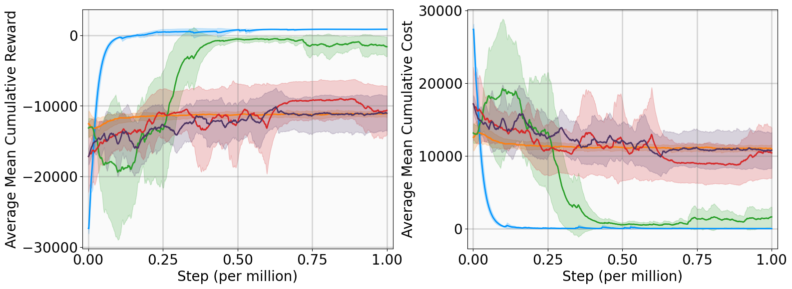
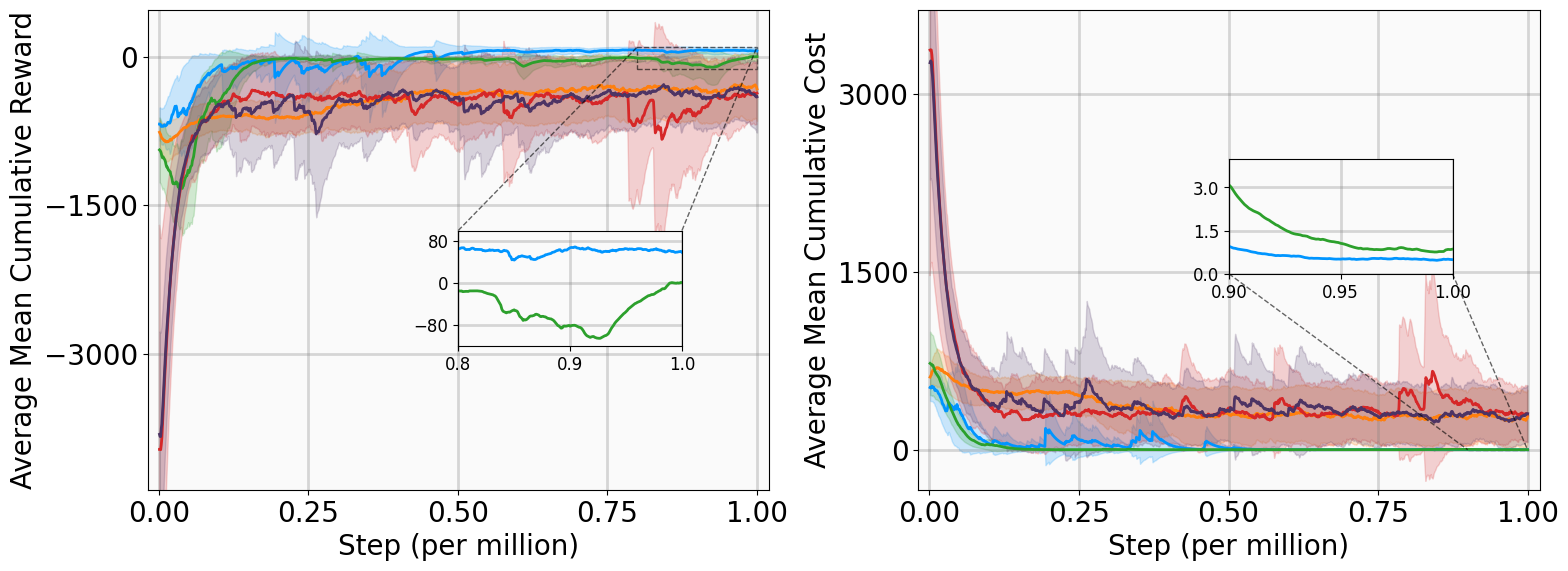
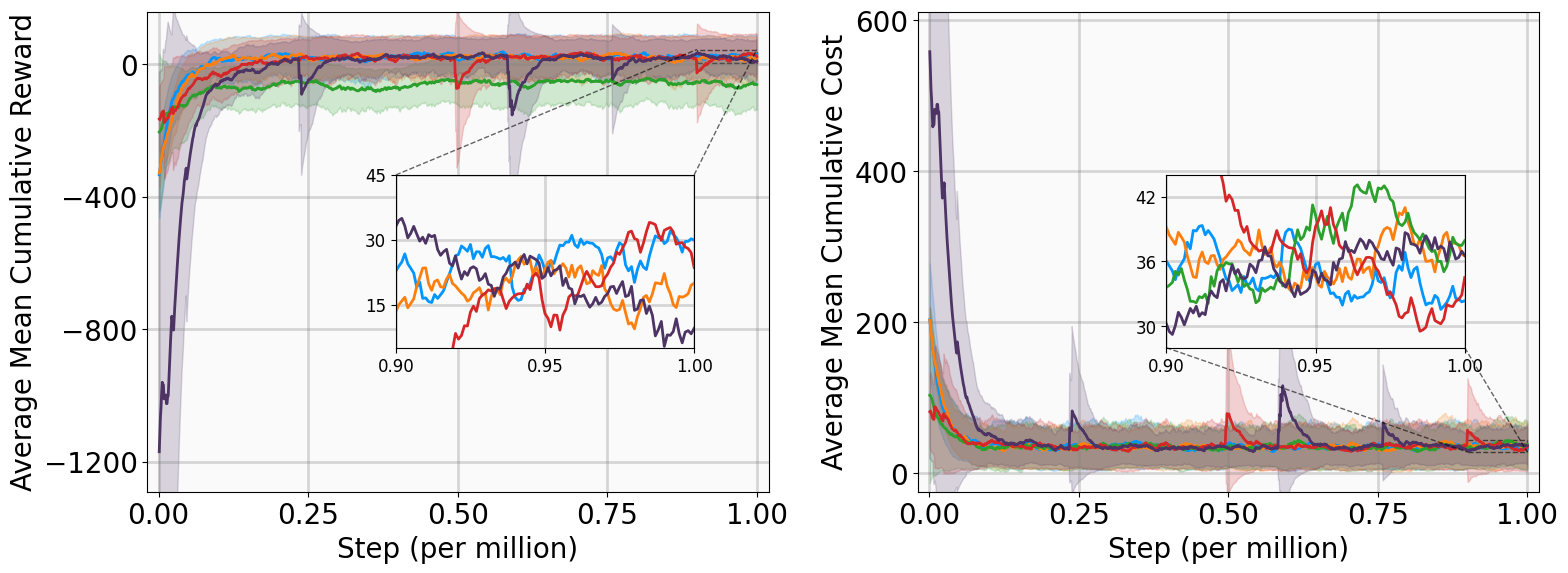
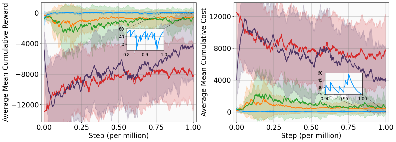
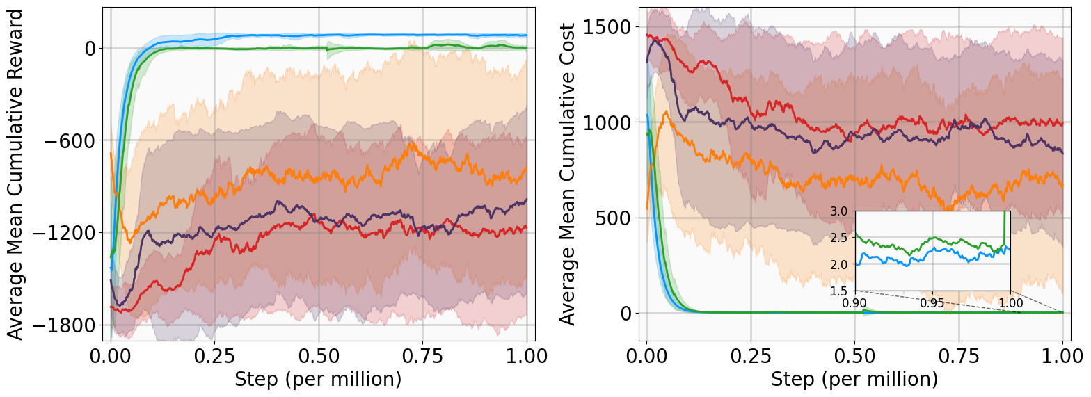
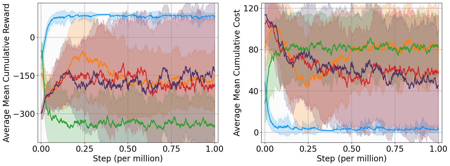
In this subsection, we present the training outcomes, evaluate stability metrics under the learned policies, and visualize the obtained Lyapunov certificates. To ensure statistical significance, each algorithm was trained using five random seeds per benchmark. The training progress is illustrated in Fig. 4, utilizing the following performance metrics:
-
AMCR (Average Mean Cumulative Reward): The sample mean of the Mean Cumulative Reward (MCR) computed across multiple independent training trials. The MCR is defined as the total undiscounted reward accumulated throughout an episode, normalized by the episode length to provide a consistent per-step measure of policy performance.
-
AMCC (Average Mean Cumulative Cost): The sample mean of the Mean Cumulative Cost (MCC) computed across multiple independent training trials. The MCC is defined as the total undiscounted cost accumulated throughout an episode, normalized by the episode length to quantify the average per-step magnitude of state deviations and control effort.
MSACL (Ours)
SAC
LAC
PPO
POLYC
The training curves demonstrate that MSACL outperforms or matches all baseline algorithms across all environments. Notably, the AMCR for MSACL remains positive and stable during the late training phase. Given our reward design, a positive MCR indicates that the system state has successfully entered the target $`\delta`$-neighborhood. Higher reward values further imply faster convergence, as the agent spends a greater proportion of the episode receiving the positive reward $`r_\delta`$.
For subsequent comparative analysis, we select the optimal policy model for each algorithm, defined as the specific model that achieved the highest MCR among the five independent training runs. These optimal policies are evaluated from 100 fixed random initial states across all benchmarks. To rigorously assess stability and convergence, we utilize the following metrics across four target radii ($`0.2, 0.1, 0.05, \text{and } 0.01`$):
-
Reach Rate (RR): The percentage of trajectories that enter the specified radius.
-
Average Reach Step (ARS): The mean number of steps required to first enter the radius.
-
Average Hold Step (AHS): The mean number of steps the state remains within the radius after the first entry.
The evaluation results are summarized in Table [algorithm_eval_metrics].
cc cc *4wc1.7cm & & & &
(lr)5-8 & & & & 0.2 & 0.1 & 0.05 & 0.01
& MSACL & 33.2 $`\pm`$ 64.5 & 31.0 $`\pm`$ 29.4 & 1.0 / 57.6 / 943.2
& 1.0 / 58.4 / 942.5 & 1.0 / 58.8 / 942.1 &
1.0 / 59.0 / 941.9
& SAC & 32.3 $`\pm`$ 64.4 & 31.1 $`\pm`$ 29.5 & 1.0 / 56.2 / 944.6 &
1.0 / 58.9 / 942.0 & 1.0 / 61.0 / 939.9 & 1.0 / 67.6 / 933.3
& LAC & 21.2 $`\pm`$ 65.1 & 31.1 $`\pm`$ 29.7 & 1.0 / 73.1 / 927.8 &
1.0 / 93.4 / 907.5 & 1.0 / 112.0 / 888.9 & 1.0 / 168.6 / 832.3
& PPO & 27.1 $`\pm`$ 64.1 & 30.8 $`\pm`$ 29.4 & 1.0 / 65.6 / 935.3 &
1.0 / 77.8 / 923.1 & 1.0 / 87.6 / 913.4 & 1.0 / 110.8 / 890.1
& POLYC & 32.3 $`\pm`$ 64.5 & 30.8 $`\pm`$ 29.4 & 1.0 / 59.3 / 941.6
& 1.0 / 61.6 / 939.3 & 1.0 / 63.2 / 937.8 & 1.0 / 66.4 / 934.5
(lr)1-8
& MSACL & 35.4 $`\pm`$ 360.1 & 30.8 $`\pm`$ 171.7 &
0.98 / 35.3 / 965.6 & 0.98 / 40.3 / 960.6 &
0.98 / 41.2 / 959.7 & 0.98 / 42.5 / 958.4
& SAC & -544.4 $`\pm`$ 1073.4 & 382.1 $`\pm`$ 640.0 &
0.74 / 34.0 / 966.8 & 0.74 / 36.0 / 964.9 & 0.74 / 37.0 / 963.9 &
0.74 / 41.6 / 959.3
& LAC & -392.6 $`\pm`$ 899.9 & 269.2 $`\pm`$ 503.4 & 0.78 / 37.6 / 963.3
& 0.78 / 51.0 / 950.0 & 0.78 / 64.6 / 936.4 & 0.78 / 111.6 / 889.4
& PPO & -6443.4 $`\pm`$ 4827.7 & 5843.8 $`\pm`$ 4912.2 & 0.0 / – / – &
0.0 / – / – & 0.0 / – / – & 0.0 / – / –
& POLYC & -2576.9 $`\pm`$ 4404.2 & 2379.5 $`\pm`$ 3986.4 &
0.69 / 27.8 / 972.4 & 0.69 / 33.6 / 967.2 & 0.69 / 37.8 / 963.1 &
0.69 / 45.4 / 955.5
(lr)1-8
& MSACL & 88.6 $`\pm`$ 3.5 & 2.1 $`\pm`$ 1.3 &
1.0 / 35.3 / 965.3 & 1.0 / 52.7 / 948.0 & 1.0 / 59.6 / 941.3
& 1.0 / 68.9 / 932.0
& SAC & -12.6 $`\pm`$ 433.8 & 81.1 $`\pm`$ 347.0 & 0.95 / 32.3 / 968.1 &
0.95 / 46.3 / 954.6 & 0.95 / 55.4 / 945.5 & 0.95 / 88.6 / 910.9
& LAC & 84.2 $`\pm`$ 4.0 & 2.0 $`\pm`$ 1.3 & 1.0 / 40.6 / 959.8 &
1.0 / 58.7 / 941.8 & 1.0 / 70.1 / 930.0 & 1.0 / 102.0 / 898.8
& PPO & -8.5 $`\pm`$ 372.7 & 73.0 $`\pm`$ 285.4 & 0.94 / 40.6 / 958.9 &
0.94 / 59.4 / 941.3 & 0.94 / 76.6 / 924.1 & 0.94 / 113.4 / 887.4
& POLYC & 82.3 $`\pm`$ 4.3 & 2.4 $`\pm`$ 1.4 & 1.0 / 44.8 / 955.3 &
1.0 / 68.7 / 932.0 & 1.0 / 87.4 / 913.1 & 1.0 / 130.5 / 870.4
(lr)1-8
& MSACL & 89.0 $`\pm`$ 7.7 & 0.4 $`\pm`$ 0.3 & 1.0 / 14.5 / 986.3 &
1.0 / 22.0 / 978.9 & 1.0 / 27.9 / 973.0 &
1.0 / 41.5 / 957.2
& SAC & -159.6 $`\pm`$ 362.5 & 179.4 $`\pm`$ 257.3 & 0.67 / 12.4 / 988.4
& 0.67 / 18.4 / 982.4 & 0.67 / 24.3 / 976.6 & 0.67 / 36.9 / 964.0
& LAC & 82.5 $`\pm`$ 8.2 & 0.3 $`\pm`$ 0.2 & 1.0 / 14.4 / 986.5
& 1.0 / 28.7 / 972.2 & 1.0 / 45.9 / 955.0 & 1.0 / 92.6 / 908.3
& PPO & -676.9 $`\pm`$ 863.7 & 472.7 $`\pm`$ 566.2 & 0.48 / 12.4 / 988.5
& 0.48 / 18.1 / 982.6 & 0.48 / 24.2 / 976.7 & 0.48 / 46.9 / 954.0
& POLYC & -172.0 $`\pm`$ 335.2 & 190.6 $`\pm`$ 246.6 &
0.60 / 14.8 / 939.0 & 0.60 / 22.8 / 978.1 & 0.60 / 28.9 / 972.0 &
0.60 / 40.2 / 960.7
(lr)1-8
& MSACL & 84.7 $`\pm`$ 32.7 & 2.9 $`\pm`$ 14.1 &
0.99 / 37.6 / 961.6 & 0.99 / 55.3 / 940.7 &
0.99 / 76.5 / 924.1 & 0.99 / 96.4 / 904.5
& SAC & 10.3 $`\pm`$ 164.9 & 21.9 $`\pm`$ 50.3 & 0.85 / 36.5 / 962.9 &
0.85 / 54.3 / 946.6 & 0.85 / 81.4 / 919.5 & 0.85 / 193.3 / 807.6
& LAC & -350.5 $`\pm`$ 196.8 & 94.5 $`\pm`$ 47.4 & 0.17 / 14.2 / 986.7 &
0.17 / 51.2 / 949.6 & 0.17 / 107.5 / 891.0 & 0.17 / 221.1 / 763.4
& PPO & 10.2 $`\pm`$ 188.6 & 21.5 $`\pm`$ 49.2 & 0.85 / 38.6 / 961.8 &
0.85 / 61.2 / 937.6 & 0.85 / 80.6 / 919.1 & 0.85 / 102.7 / 894.4
& POLYC & 40.1 $`\pm`$ 152.8 & 14.7 $`\pm`$ 39.9 & 0.90 / 34.9 / 962.0 &
0.90 / 58.0 / 939.8 & 0.90 / 67.6 / 932.3 & 0.90 / 81.8 / 912.3
(lr)1-8
& MSACL & 838.8 $`\pm`$ 1.5 & 14.5 $`\pm`$ 2.1 &
1.0 / 33.1 / 967.8 & 1.0 / 34.0 / 966.9 & 1.0 / 36.9 / 964.0
& 1.0 / 49.7 / 619.8
& SAC & -17263.8 $`\pm`$ 1380.0 & 17246.4 $`\pm`$ 1379.1 & 0.0 / – / – &
0.0 / – / – & 0.0 / – / – & 0.0 / – / –
& LAC & -51.1 $`\pm`$ 1.2 & 32.7 $`\pm`$ 1.1 & 1.0 / 471.9 / 20.6 &
0.0 / – / – & 0.0 / – / – & 0.0 / – / –
& PPO & -12836.6 $`\pm`$ 4042.3 & 12571.3 $`\pm`$ 4022.4 & 0.0 / – / – &
0.0 / – / – & 0.0 / – / – & 0.0 / – / –
& POLYC & -17528.1 $`\pm`$ 2162.6 & 17318.7 $`\pm`$ 2155.6 & 0.0 / – / –
& 0.0 / – / – & 0.0 / – / – & 0.0 / – / –
Note: The values for AMCR and AMCC represent the mean performance of the optimal policy (defined as the policy achieving the highest evaluation MCR) averaged over 100 independent trials, with $`\pm`$ denoting one standard deviation. Stability metrics (RR, ARS, and AHS) are evaluated across four distinct radii, where “–” indicates that the system failed to enter the specified radius within the episode duration. Bold entries highlight the superior results: for performance metrics, the maximum AMCR and minimum AMCC are bolded; for stability metrics, the highest RR is prioritized for bolding, with the shortest ARS and longest AHS selected in the event of identical RR values.
These results highlight the superiority of MSACL. Across all six environments, MSACL consistently achieves the highest AMCR. In terms of AMCC, MSACL attains the absolute minimum in the Pendulum, SingleTrackCar, and QuadrotorTracking tasks, while remaining highly competitive in others. Furthermore, MSACL achieves the highest RR across all radii. Most significantly, in the high-dimensional nonlinear QuadrotorTracking task, MSACL is the only method to achieve a 100% reach rate at the $`0.01`$ precision level, whereas baselines fail to meet this stringent requirement. These results underscore the robustness and precision of MSACL in complex control applications.
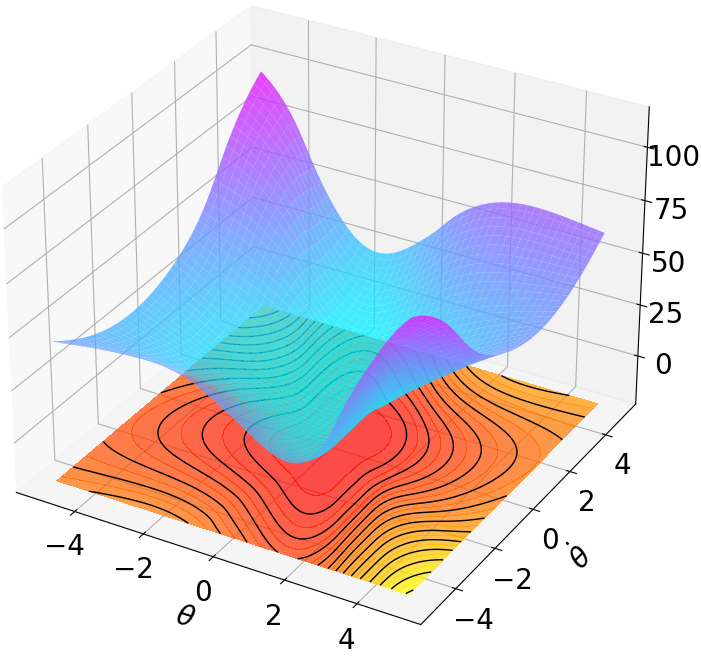
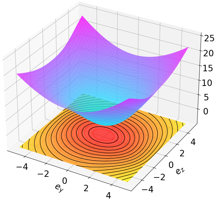
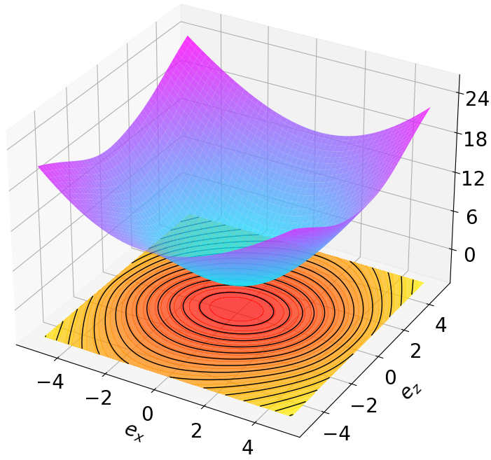
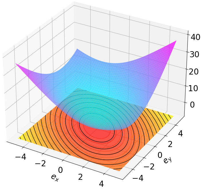
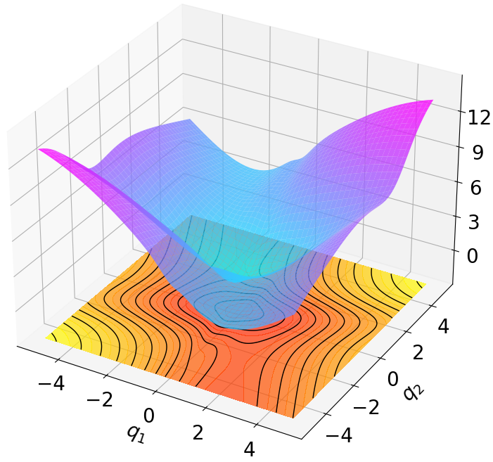
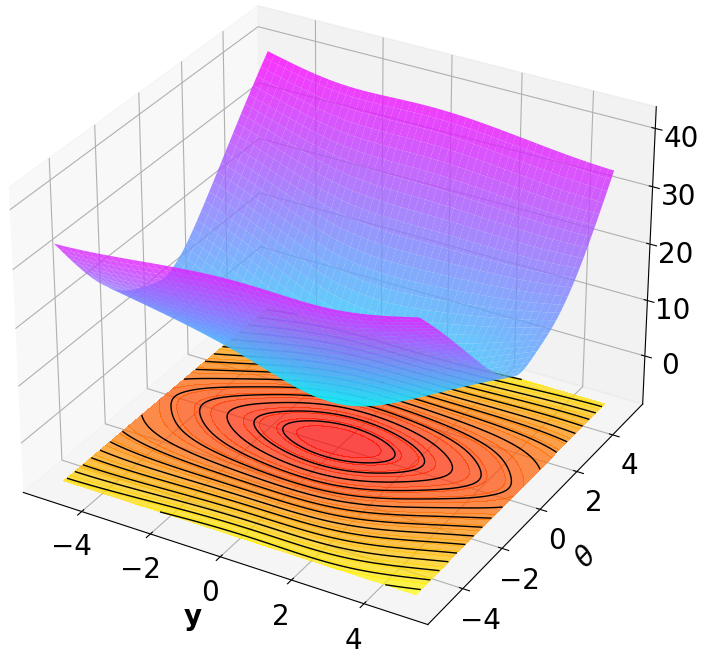
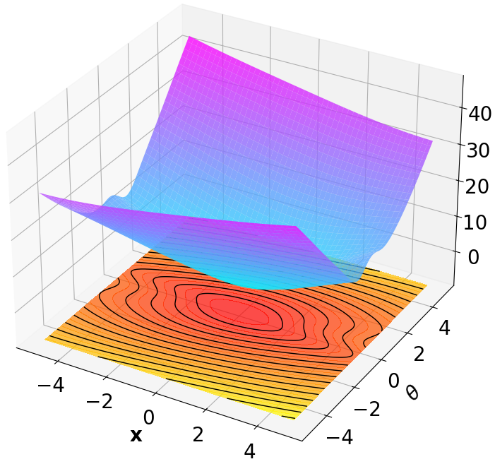
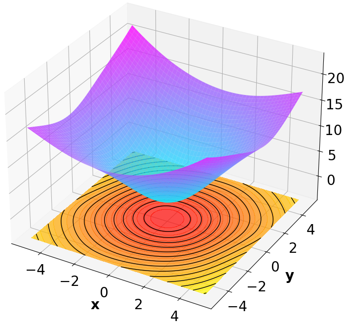
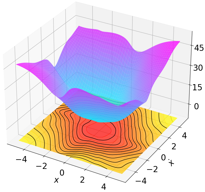
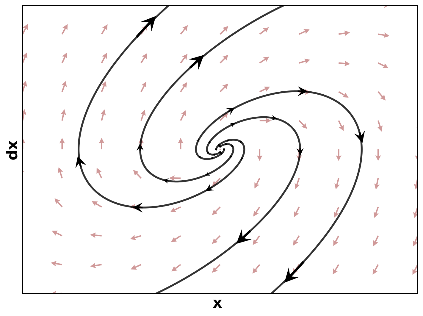
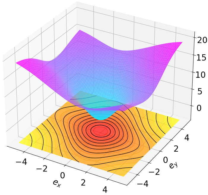
Finally, we visualize the Lyapunov networks $`V_\psi`$ corresponding to the optimal policies. The learned Lyapunov certificates and their associated contour plots are shown in Fig. 5. For high-dimensional systems, the plots represent the relationship between $`V_\psi`$ and two specific state components while setting all other components to zero.
Remark 4. Since MSACL is built upon the SAC framework, SAC serves as the primary baseline for our ablation study. As shown in Fig. 4 and Table [algorithm_eval_metrics], the integration of the Lyapunov certificate significantly enhances both training performance and stability metrics compared to the standard SAC algorithm. This validates that embedding Lyapunov-based constraints into maximum entropy RL effectively yields neural policies with superior stability guarantees for deterministic control systems.
Evaluation of Robustness and Generalization
It is well known that neural policies, characterized by high-dimensional parameter spaces, are susceptible to overfitting within specific training environments. This can lead to degraded robustness against stochastic noise and parametric variations, as well as limited generalization to unseen scenarios. In this subsection, we evaluate the robustness and generalization capabilities of the policies trained via MSACL to demonstrate their applicability in real-world environments with inherent uncertainties.
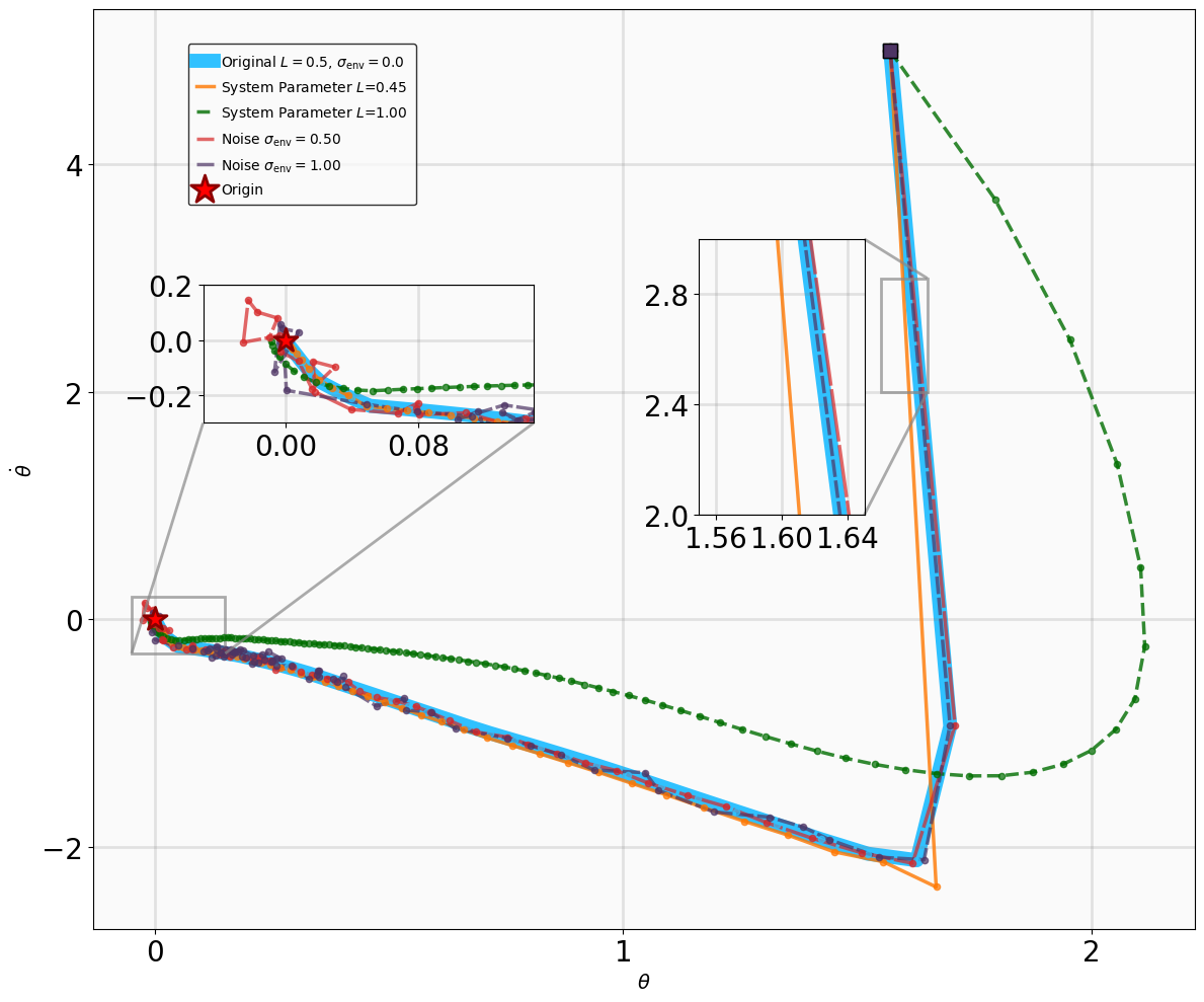
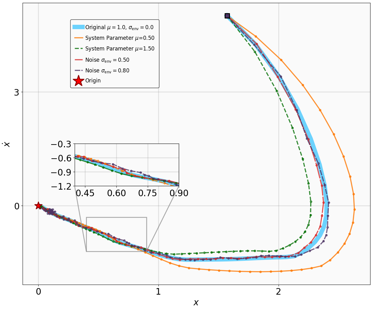
For stabilization tasks (VanderPol, Pendulum, DuctedFan, and Two-link), we introduce process noise $`\boldsymbol{\epsilon}_t \sim \mathcal{N}(\mathbf{0}, \boldsymbol{\sigma}_{\text{env}})`$ to the system dynamics, resulting in the perturbed form:
\begin{equation*}
    \mathbf{x}_{t+1} = f(\mathbf{x}_t, \mathbf{u}_t) + \boldsymbol{\epsilon}_t.
\end{equation*}Additionally, we modify key physical parameters of the systems to assess whether the MSACL-trained policies can maintain stability under environmental variations.
For tracking tasks (SingleCarTracking and QuadrotorTracking), we evaluate robustness by injecting dynamical noise and assess generalization by requiring the policies to track reference trajectories $`\mathbf{x}_t^{\text{ref}}`$ that differ significantly from those encountered during training. The specific parameter modifications and noise magnitudes utilized for these evaluations are detailed in Table 2.
| Benchmarks | System Parameters | Noise Magnitude ($`\sigma_{\mathrm{env}}`$) |
|---|---|---|
| VanderPol | $`\mu = 0.5, 1.5`$ | $`0.5, 0.8`$ |
| Pendulum | $`L = 0.5, 1.0`$ | $`0.5, 1.0`$ |
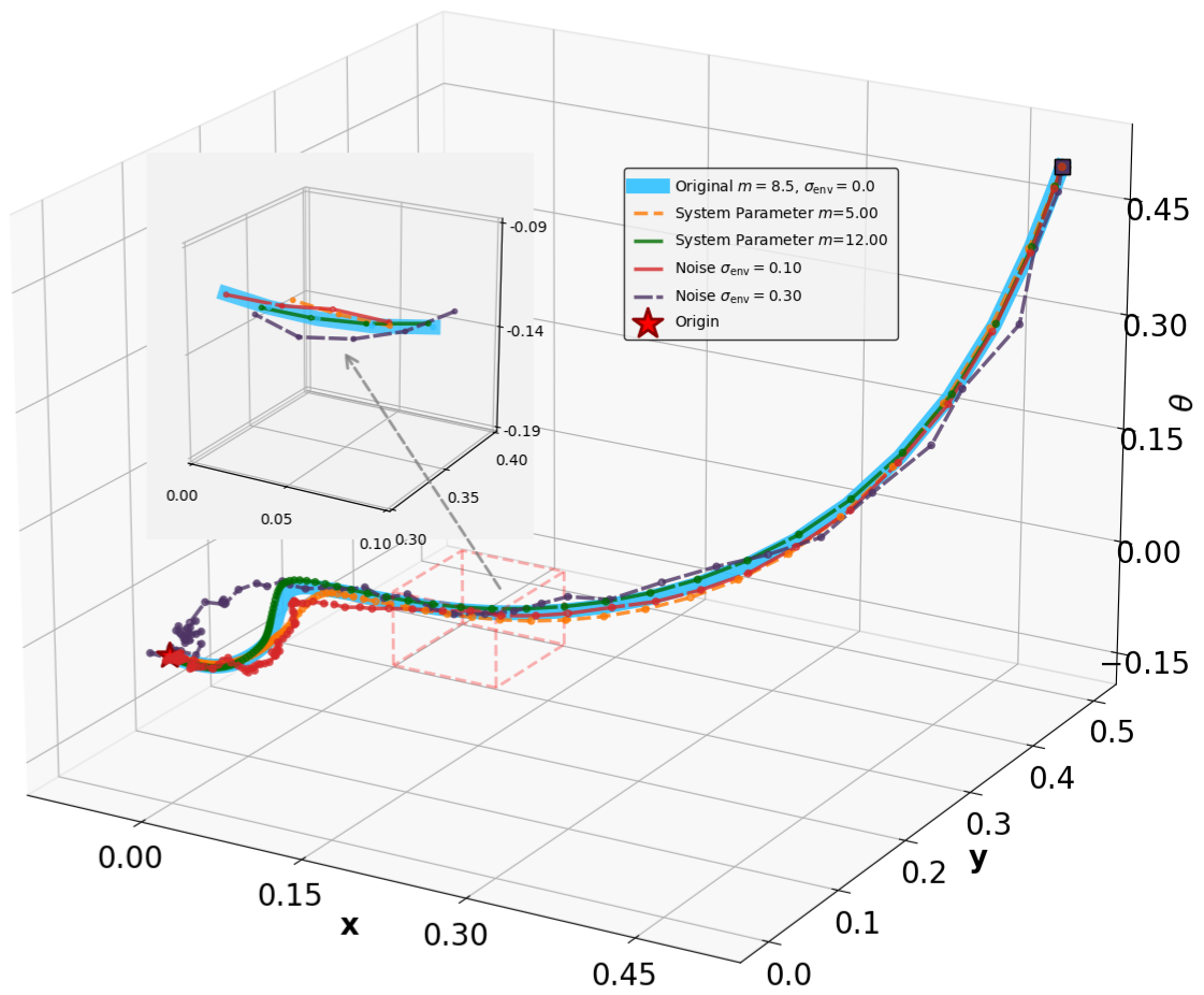
| DuctedFan | $`m = 5, 12`$ | $`0.1, 0.3`$ |
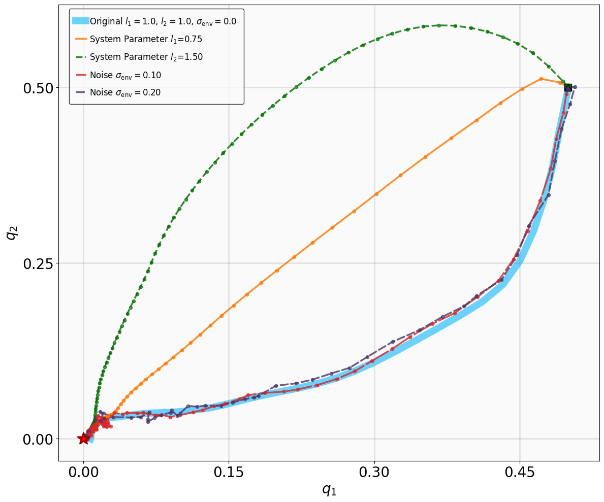
| Two-link | $`l_1 = 0.75, l_2 = 1.5`$ | $`0.1, 0.2`$ |
| SingleCarTracking | – | $`0.1, 0.3`$ |
| QuadrotorTracking | – | $`0.01, 0.02`$ |
System Parameters and Noise Magnitudes
The robustness testing results for the stabilization tasks are illustrated in Fig. 6. Despite the introduction of parametric perturbations and process noise, all system trajectories originating from the specified initial states successfully converge to the neighborhood of the equilibrium $`\mathbf{x}_g = \mathbf{0}`$.
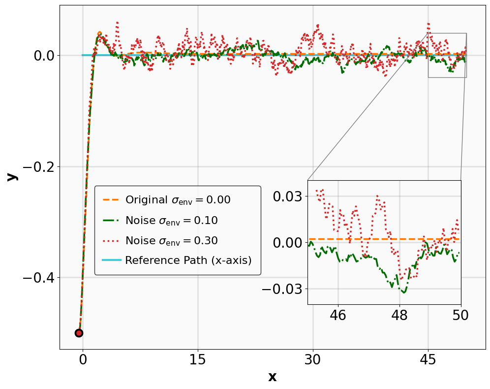
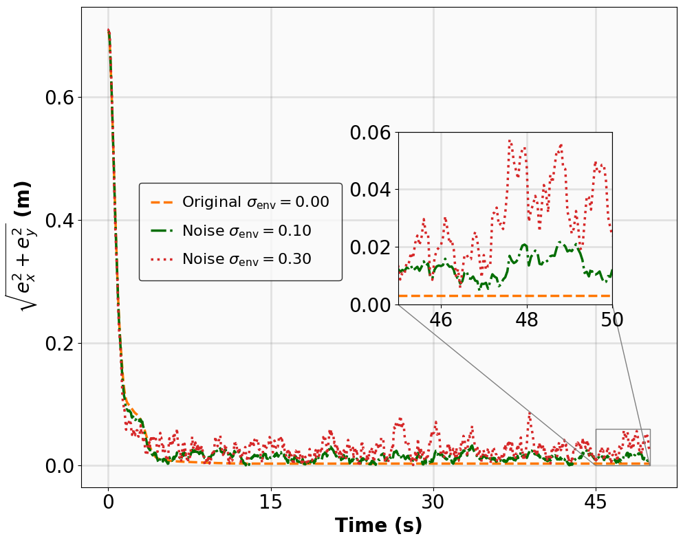
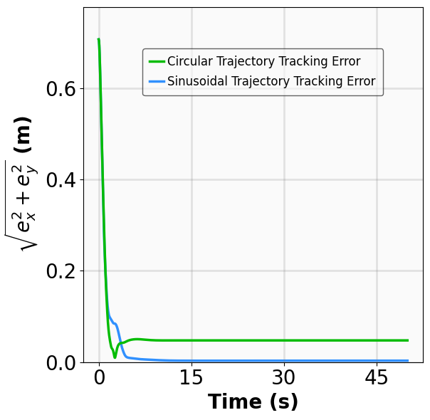
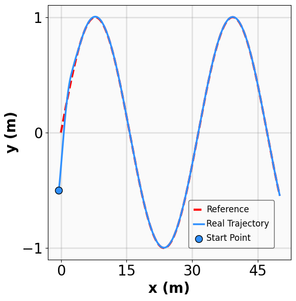
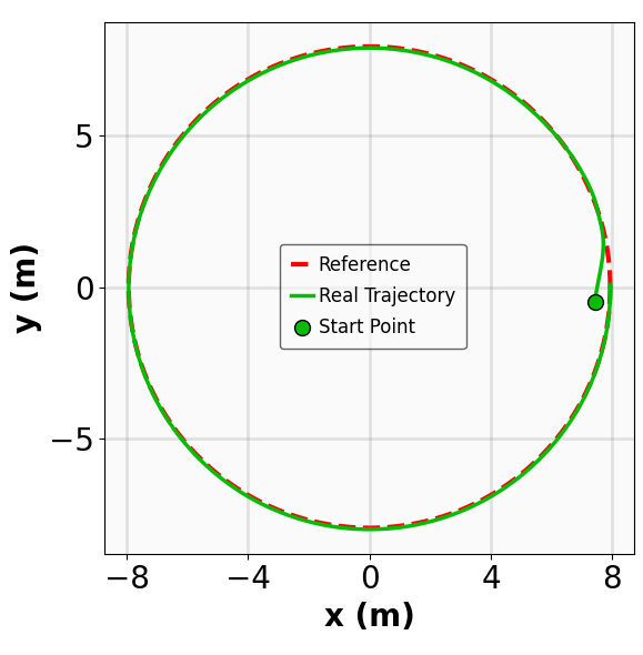
The results for the tracking tasks are presented in Fig. 7 and Fig. 8. It is evident that the trained neural policies effectively mitigate noise interference within a reasonable range. In the SingleCarTracking environment, while the policy was trained on straight-line references, we evaluate its generalization using circular and sinusoidal trajectories. Experimental validation demonstrates excellent tracking performance; as shown in the position error plot in Fig. [general-STCar-3], the tracking error $`e_{\mathrm{xy}} = \sqrt{e_x^2 + e_y^2}`$ remains within 0.1 during the steady-state phase.
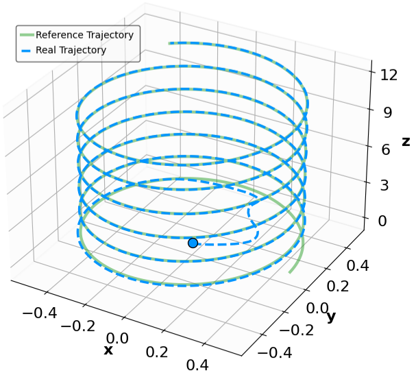
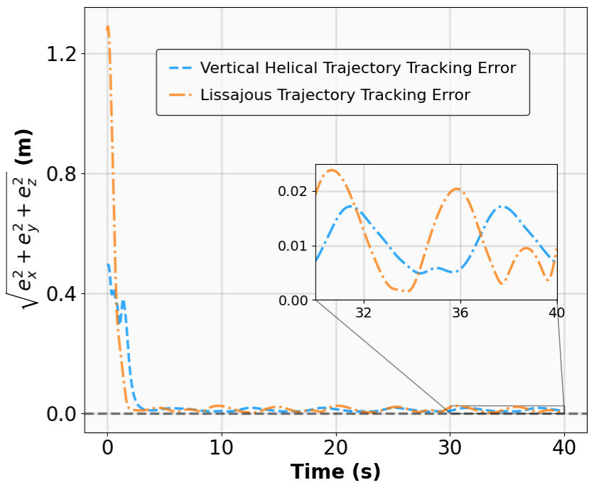
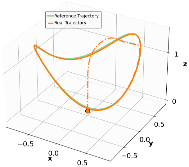
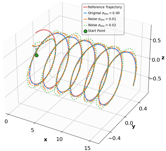
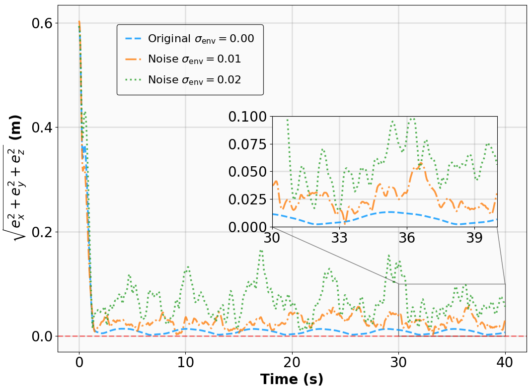
For the QuadrotorTracking task, the policy was trained using a horizontal helical trajectory. During generalization testing, we evaluate the policy against two unseen trajectories: a vertical helix and a Lissajous curve, as shown in Fig. [general-Quad-1] and Fig. [general-Quad-2]. Notably, the MSACL-trained policy demonstrates superior generalization, with the tracking error $`e_{\mathrm{xyz}} = \sqrt{e_x^2 + e_y^2 + e_z^2}`$ stabilizing around 0.02 in the later stages.
Based on these results, we conclude that policies trained via the MSACL algorithm exhibit robust performance against moderate uncertainties and favorable generalization to unseen reference trajectories. However, our testing also reveals that the policies’ efficacy diminishes under extreme disturbances or environmental parameters that deviate substantially from the training distribution. In such cases of significant domain shift, the MSACL algorithm can be readily redeployed to retrain the policy, ensuring stable and high-precision control for the specific operational scenario.
Sensitivity Analysis of the Multi-Step Horizon $`n`$
In this subsection, we investigate the influence of the multi-step horizon parameter $`n`$ on the performance of the MSACL algorithm across all benchmark environments. Following the evaluation protocol detailed in Section 5.3, we utilize both performance metrics (AMCR and AMCC) and stability metrics (RR, ARS, and AHS) to assess the policies trained under varying configurations of $`n`$. Specifically, we conduct 100 randomized experiments for each benchmark by generating and fixing a set of 100 random initial states. Policies trained with different $`n`$ values interact with the environment starting from these fixed states to compute the aforementioned evaluation metrics.
The results across all environments are summarized in Table [n_step_results]. The experimental findings reveal a consistent trend: as $`n`$ increases, the stabilization and tracking performance of the MSACL-trained policies generally improves. This improvement occurs because a larger $`n`$ provides a longer-horizon trajectory during training, enabling the policy $`\pi`$ to more accurately identify the stability direction, namely the descent direction of the Lyapunov certificate $`V_\psi`$. This reduces the training bias and reinforces the stability guarantees for the resulting neural policy.
Empirically, setting $`n=20`$ yields satisfactory performance across all benchmark environments, suggesting it as a versatile default parameter. However, an excessively large $`n`$ may not always lead to optimal results. As analyzed in Section 3.2, longer temporal horizons introduce greater cumulative variance into the training data, which can distort the optimization landscape and result in suboptimal policies. Therefore, selecting an appropriate $`n`$ is essential to balancing the bias-variance trade-off. In summary, for the control tasks presented in this article, $`n=20`$ delivers consistently robust results; for specific applications requiring peak performance, fine-tuning around this value is recommended to achieve the optimal balance between training bias and variance.
cc cc *4wc1.7cm & & & &
(lr)5-8 & & & & 0.2 & 0.1 & 0.05 & 0.01
& $`n=1`$ & 30.2 $`\pm`$ 64.5 & 31.1 $`\pm`$ 29.5 & 1.0 / 56.3 / 944.6 &
1.0 / 61.9 / 939.0 & 1.0 / 68.9 / 932.0 & 1.0 / 88.2 / 912.7
& $`n=5`$ & 31.5 $`\pm`$ 64.5 & 30.9 $`\pm`$ 29.4 &
1.0 / 58.4 / 942.4 & 1.0 / 63.4 / 937.5 & 1.0 / 67.6 / 933.3 &
1.0 / 78.7 / 922.2
& $`n=10`$ & 32.4 $`\pm`$ 64.6 & 30.9 $`\pm`$ 29.4 &
1.0 / 57.9 / 942.9 & 1.0 / 61.4 / 939.5 & 1.0 / 64.1 / 936.8 &
1.0 / 68.9 / 932.0
& $`n=15`$ & 33.1 $`\pm`$ 64.4 & 31.2 $`\pm`$ 29.5 &
1.0 / 54.1 / 946.7 & 1.0 / 55.1 / 945.8 & 1.0 / 55.7 / 945.3
& 1.0 / 57.0 / 943.9
& $`n=20`$ & 33.2 $`\pm`$ 64.5 & 31.0 $`\pm`$ 29.5 &
1.0 / 57.8 / 943.1 & 1.0 / 58.7 / 942.2 & 1.0 / 59.2 / 941.7 &
1.0 / 59.5 / 941.4
(lr)1-8
& $`n=1`$ & -578.5 $`\pm`$ 1232.9 & 444.2 $`\pm`$ 815.1 &
0.77 / 37.1 / 963.5 & 0.77 / 42.4 / 958.6 & 0.77 / 44.4 / 956.5 &
0.77 / 48.8 / 952.1
& $`n=5`$ & 34.7 $`\pm`$ 360.0 & 30.7 $`\pm`$ 171.8 &
0.98 / 36.8 / 964.0 & 0.98 / 44.7 / 956.2 & 0.98 / 46.0 / 954.9 &
0.98 / 49.4 / 951.5
& $`n=10`$ & 35.7 $`\pm`$ 360.1 & 31.0 $`\pm`$ 171.7 &
0.98 / 34.9 / 966.0 & 0.98 / 35.6 / 965.4 &
0.98 / 36.1 / 964.9 & 0.98 / 38.5 / 962.3
& $`n=15`$ & 35.2 $`\pm`$ 360.0 & 31.0 $`\pm`$ 171.7 &
0.98 / 35.2 / 965.6 & 0.98 / 36.9 / 964.0 & 0.98 / 38.4 / 962.6 &
0.98 / 44.0 / 956.9
& $`n=20`$ & 35.8 $`\pm`$ 355.7 & 30.3 $`\pm`$ 167.9 &
0.98 / 38.0 / 962.8 & 0.98 / 39.3 / 961.6 & 0.98 / 40.7 / 960.2 &
0.98 / 44.1 / 956.8
(lr)1-8
& $`n=1`$ & -116.3 $`\pm`$ 584.8 & 163.2 $`\pm`$ 463.3 &
0.89 / 32.3 / 967.8 & 0.89 / 49.8 / 950.6 & 0.89 / 57.0 / 943.9 &
0.89 / 83.5 / 917.3
& $`n=5`$ & 87.4 $`\pm`$ 3.7 & 2.0 $`\pm`$ 1.3 & 1.0 / 35.5 / 965.2
& 1.0 / 49.8 / 950.9 & 1.0 / 57.9 / 942.9 & 1.0 / 78.4 / 922.1
& $`n=10`$ & 88.6 $`\pm`$ 3.5 & 2.1 $`\pm`$ 1.3 &
1.0 / 35.3 / 965.3 & 1.0 / 52.7 / 948.0 & 1.0 / 59.6 / 941.3 &
1.0 / 68.9 / 932.0
& $`n=15`$ & 88.1 $`\pm`$ 4.0 & 2.0 $`\pm`$ 1.3 & 1.0 / 36.1 / 964.6
& 1.0 / 52.0 / 949.0 & 1.0 / 61.4 / 939.5 & 1.0 / 74.3 / 926.6
& $`n=20`$ & 73.7 $`\pm`$ 37.7 & 4.4 $`\pm`$ 8.5 & 0.95 / 56.3 / 944.2 &
0.95 / 79.2 / 921.6 & 0.95 / 94.5 / 906.4 & 0.95 / 127.0 / 873.9
(lr)1-8
& $`n=1`$ & -208.6 $`\pm`$ 372.5 & 216.0 $`\pm`$ 267.0 &
0.60 / 13.8 / 987.2 & 0.60 / 22.3 / 976.7 & 0.60 / 29.6 / 971.3 &
0.60 / 40.4 / 960.5
& $`n=5`$ & -142.4 $`\pm`$ 340.0 & 167.6 $`\pm`$ 241.6 &
0.67 / 13.7 / 987.0 & 0.67 / 20.3 / 980.4 & 0.67 / 24.7 / 976.1 &
0.67 / 29.9 / 971.0
& $`n=10`$ & -163.8 $`\pm`$ 346.6 & 183.1 $`\pm`$ 247.1 &
0.64 / 10.7 / 990.2 & 0.64 / 16.4 / 984.5 & 0.64 / 23.2 / 977.6 &
0.64 / 37.0 / 963.9
& $`n=15`$ & -131.0 $`\pm`$ 354.1 & 158.3 $`\pm`$ 251.4 &
0.71 / 12.1 / 988.7 & 0.71 / 18.5 / 982.3 & 0.71 / 24.8 / 976.1 &
0.71 / 40.6 / 960.3
& $`n=20`$ & 89.8 $`\pm`$ 7.5 & 0.4 $`\pm`$ 0.2 &
1.0 / 18.1 / 982.0 & 1.0 / 25.0 / 975.8 & 1.0 / 28.6 / 972.2
& 1.0 / 35.2 / 965.7
(lr)1-8
& $`n=1`$ & -51.0 $`\pm`$ 194.9 & 46.4 $`\pm`$ 62.6 &
0.64 / 32.0 / 964.0 & 0.64 / 64.6 / 931.1 & 0.64 / 79.7 / 921.2 &
0.64 / 92.1 / 908.8
& $`n=5`$ & -40.2 $`\pm`$ 217.9 & 35.0 $`\pm`$ 58.8 &
0.74 / 31.6 / 968.7 & 0.74 / 56.1 / 943.8 & 0.74 / 78.9 / 920.9 &
0.74 / 113.0 / 887.8
& $`n=10`$ & 84.7 $`\pm`$ 32.7 & 2.9 $`\pm`$ 14.1 &
0.99 / 37.6 / 961.6 & 0.99 / 55.3 / 940.7 &
0.99 / 76.5 / 924.1 & 0.99 / 96.4 / 904.5
& $`n=15`$ & 67.5 $`\pm`$ 84.7 & 8.8 $`\pm`$ 32.5 & 0.95 / 35.2 / 964.8
& 0.95 / 57.8 / 938.7 & 0.95 / 82.6 / 917.0 & 0.95 / 109.1 / 891.7
& $`n=20`$ & 82.6 $`\pm`$ 55.1 & 3.0 $`\pm`$ 15.6 & 0.99 / 37.6 / 960.5
& 0.99 / 63.1 / 934.3 & 0.99 / 85.0 / 915.8 & 0.99 / 95.0 / 905.6
(lr)1-8
& $`n=1`$ & -12708.9 $`\pm`$ 645.4 & 12582.7 $`\pm`$ 645.2 & 0.0 / – / –
& 0.0 / – / – & 0.0 / – / – & 0.0 / – / –
& $`n=5`$ & -4708.7 $`\pm`$ 3158.6 & 4646.3 $`\pm`$ 3135.9 & 0.0 / – / –
& 0.0 / – / – & 0.0 / – / – & 0.0 / – / –
& $`n=10`$ & 534.3 $`\pm`$ 5.0 & 11.8 $`\pm`$ 0.9 & 1.0 / 54.4 / 946.5 &
1.0 / 66.2 / 934.7 & 1.0 / 116.5 / 650.9 & 0.0 / – / –
& $`n=15`$ & 858.5 $`\pm`$ 1.0 & 10.8 $`\pm`$ 0.5 &
1.0 / 31.3 / 969.6 & 1.0 / 36.8 / 964.1 & 1.0 / 41.2 / 959.7 &
1.0 / 115.4 / 747.9
& $`n=20`$ & 838.5 $`\pm`$ 1.5 & 14.7 $`\pm`$ 2.0 & 1.0 / 33.1 / 967.8 &
1.0 / 34.1 / 966.8 & 1.0 / 37.0 / 963.9 &
1.0 / 49.8 / 620.0
Discussion and Conclusion
Discussion
This subsection provides an analytical discussion on the functional roles of the various components within the MSACL framework. As highlighted in Remark 4, MSACL extends the Soft Actor-Critic (SAC) algorithm by integrating multi-step Lyapunov certificate learning, thereby establishing formal stability guarantees while preserving the exploration efficiency of maximum entropy reinforcement learning. In model-free stabilization and tracking tasks, conventional SAC, which lacks the structural guidance provided by Lyapunov theory, may fail to converge to stable policies under improper reward structures. Even with well-designed rewards, standard RL often requires exhaustive exploration of the action space to identify stabilizing directions, leading to prohibitive training times. To address these limitations, our approach introduces a Lyapunov network that serves as a stability-oriented critic, providing explicit directional guidance during policy updates by identifying action sequences that facilitate the descent of the Lyapunov certificate.
The theoretical foundation of this mechanism is rooted in Lemma 1, which establishes the equivalence between the Lyapunov stability conditions and exponential state convergence. To ensure the Lyapunov certificate $`V_\psi`$ is learned accurately, we developed a training methodology that aligns theoretical requirements with empirical trajectories. Specifically, the introduction of Exponential Stability Labels (ESL) in Definition 2 allows the algorithm to categorize trajectory segments as positive or negative samples based on their adherence to exponential decay criteria. This classification enables the construction of the loss function ([loss_diff_V]), which effectively bridges abstract stability conditions with observed system dynamics.
The policy optimization process leverages this learned certificate through the stability advantage mechanism defined in ([loss_policy]). This advantage function quantifies the rate of Lyapunov descent along trajectories, prioritizing policy updates that simultaneously ensure stability and accelerate convergence. Our experimental results confirm that this dual-objective optimization yields policies that achieve both stability and rapid convergence across diverse and challenging benchmarks. A critical insight is that the efficacy of the policy is fundamentally tied to the fidelity of the learned Lyapunov certificate. The multi-step sampling strategy, combined with the ESL-based loss formulation, ensures that $`V_\psi`$ accurately reflects the theoretical stability criteria, providing reliable gradients for policy improvement.
While developed for stabilization and tracking, the MSACL framework is highly extensible to other stability-critical applications. Potential extensions include trajectory planning for autonomous vehicles , spacecraft proximity operations , and robotic manipulation tasks requiring rigorous safety guarantees . The integration of Lyapunov-based guarantees within maximum entropy RL represents a significant step toward developing verifiable, learning-based control systems for real-world deployment.
Conclusion
This article presented the MSACL (Multi-Step Actor-Critic Learning with Lyapunov certificates) algorithm, a novel framework that integrates exponential stability guarantees into the maximum entropy RL paradigm. By embedding Lyapunov stability theory within the SAC architecture, MSACL achieves stable control for model-free dynamical systems without sacrificing the exploration benefits of entropy regularization.
To rigorously evaluate the proposed methodology, we developed six benchmark environments covering four stabilization and two tracking tasks. Comprehensive comparisons against established baselines demonstrate the consistent superiority of MSACL across both performance and stability metrics. Notably, these results were achieved using a simple reward structure that penalizes state deviations and control effort while providing sparse positive rewards near the equilibrium. Beyond standard performance, we conducted extensive robustness analyses against environmental uncertainties and generalization tests on unseen reference trajectories. The MSACL-trained neural policies exhibited remarkable resilience to disturbances and effective adaptation to geometrically distinct paths.
A key algorithmic contribution is the systematic analysis of the multi-step horizon parameter $`n`$. We established that $`n=20`$ serves as a robust default setting, effectively balancing the bias-variance trade-off in stability learning. This work advances the integration of formal stability guarantees within learning-based control, providing a foundation for verifiable policies in safety-critical applications. Future research will explore extensions to partially observable systems , adaptive Lyapunov architectures , and transfer learning mechanisms for complex, cross-domain dynamical systems .
This appendix provides a detailed description of the six nonlinear dynamical systems selected as benchmarks for this study: VanderPol, Pendulum, DuctedFan, Two-link, SingleCarTracking, and QuadrotorTracking. Widely recognized as canonical benchmarks in nonlinear control (NLC) , reinforcement learning (RL) , and optimal control literature , these environments constitute a comprehensive testbed for evaluating the proposed methods. They encompass a broad spectrum of dynamic characteristics, ranging from self-sustaining oscillations and underactuated mechanics to complex tire–road friction interactions and rigid-body dynamics on the $`\text{SE}(3)`$ manifold.
To provide a unified evaluation framework, we categorize these benchmarks based on their control objectives: Stabilization and Tracking. The formal task definitions and their corresponding reward structures are detailed below.
Unified Control Objectives
Despite the distinct physical dynamics inherent to each system, the core control tasks are formulated using a consistent mathematical structure.
Stabilization Tasks
The first four systems (VanderPol, Pendulum, DuctedFan, and Two-link) are configured as stabilization tasks. For these systems, the control objective is to find a policy that generates a sequence of control inputs $`\{\mathbf{u}_t\}_{t=0}^{T-1}`$ to drive the system state $`\mathbf{x}_t`$ from a randomly sampled initial state $`\mathbf{x}_0`$ toward a fixed equilibrium point $`\mathbf{x}_g`$ (typically the origin, $`\mathbf{x}_g = \mathbf{0}`$) and maintain stability at this equilibrium for the duration of the episode.
Tracking Tasks
The remaining two systems (SingleCarTracking, and QuadrotorTracking) are formulated as trajectory tracking tasks. Here, the objective is defined in terms of the tracking error $`\mathbf{e}_t = \mathbf{x}_t - \mathbf{x}_t^{\text{ref}}`$. The goal is to determine a control sequence such that the error trajectory $`\{\mathbf{e}_t\}_{t=0}^{T}`$ converges to the zero-error state $`\mathbf{e}_g = \mathbf{0}`$, thereby ensuring that the system state $`\mathbf{x}_t`$ accurately follows a time-varying reference trajectory $`\mathbf{x}_t^{\text{ref}}`$.
Unified Reward Function Design
To align the learning process with the aforementioned control objectives, we employ a consistent reward function structure across all six environments:
\begin{equation*}
r_t = \underbrace{-\left(\mathbf{s}_t^\top \mathbf{Q}_r \mathbf{s}_t + \mathbf{u}_t^\top \mathbf{R}_r \mathbf{u}_t\right)}_{\text{Penalty}} + \underbrace{r_{\text{approach}}(\mathbf{s}_t)}_{\text{Encouragement}},
\label{eq:unified_reward}
\end{equation*}where $`\mathbf{s}_t`$ represents the generalized state vector, defined as $`\mathbf{s}_t = \mathbf{x}_t`$ for stabilization tasks and $`\mathbf{s}_t = \mathbf{e}_t`$ for tracking tasks. The matrices $`\mathbf{Q}_r`$ and $`\mathbf{R}_r`$ are positive semi-definite weighting matrices that penalize state deviations and control effort, respectively.
The specific parameter configurations for each environment, including the diagonal elements of $`\mathbf{Q}_r`$ and $`\mathbf{R}_r`$, are summarized in Table [tab:reward_params]. The term $`\mathbb{I}(\cdot)`$ denotes the indicator function, which provides a sparse encouragement reward when the system enters a predefined tolerance region around the target state. For all environments, the state cost matrix $`\mathbf{Q}_c`$ is simply defined as a identity matrix $`\mathbf{I}_n`$ of appropriate dimensions, where $`n`$ denotes the dimension of state space.
Details of VanderPol
System Overview
The VanderPol oscillator, originally proposed by Balthasar van der Pol in 1920 , is a classic model describing self-sustaining oscillatory circuits characterized by nonlinear damping. This system serves as a fundamental benchmark for electronic circuit stabilization (e.g., vacuum tube oscillators), mechanical vibration control, and biological modeling, such as cardiac pacemaker dynamics . In this study, we extend the autonomous system with a control input to evaluate stabilization performance within a nonlinear regime.
Dynamics and Physical Parameters
The continuous-time dynamics of controlled VanderPol are governed by the following second-order nonlinear differential equations:
\begin{align*}
    \dot{x}_1 &= x_2, \\
    \dot{x}_2 &= \mu \left(1 - x_1^2\right) x_2 - x_1 + u,
\end{align*}where $`x_1`$ and $`x_2`$ represent the oscillator displacement and velocity, respectively. The physical meanings of the variables are summarized in Table 3, and the specific parameter values and simulation settings used in our experiments are detailed in Table 4.
| Variable | Physical Meaning |
|---|---|
| $`x_1`$ | Displacement of the oscillator (m) |
| $`x_2`$ | Velocity of the oscillator (m/s) |
| $`\dot{x}_2`$ | Acceleration of the oscillator (m/s$`^2`$) |
| $`\mu`$ | Nonlinear damping strength parameter (dimensionless) |
| $`u`$ | Control input force applied to the oscillator (N) |
Variable Definitions for Controlled VanderPol
| Parameter | Value |
|---|---|
| $`\mu`$ (nonlinear strength) | 1.0 (dimensionless) |
| Simulation time step ($`dt`$) | 0.01 s |
| Control update interval | 5 simulation steps |
| Maximum episode steps | 1000 |
Parameter Values for Controlled VanderPol
State and Action Spaces
For the reinforcement learning formulation, the system state vector is defined as $`\mathbf{x} = [x_1, x_2]^\top`$. To reflect the physical limits of the oscillator and ensure numerical stability during training, the state space is constrained to $`\mathcal{X} = [-10, 10] \times [-10, 10]`$, where both displacement and velocity are bounded within the range of $`\pm 10`$. The control objective is to drive the system from a random initial configuration to the equilibrium state (goal state) defined as $`\mathbf{x}_g = [0, 0]^\top`$, corresponding to the stable origin of the phase plane.
The control action $`u`$ is a one-dimensional continuous input restricted to the action space $`\mathcal{U} = [-5, 5]`$. These bounds are selected to provide sufficient authority for stabilization while preventing excessively large inputs that could violate physical actuation constraints or lead to divergent gradients. At the start of each episode, the initial state $`\mathbf{x}_0`$ is sampled from a uniform distribution $`\mathbf{x}_0 \sim \text{Uniform}([-5, 5] \times [-5, 5])`$. This initialization range is intentionally chosen to place the system within a significant nonlinear regime, ensuring that the controller must actively counteract the self-sustaining oscillations to achieve stabilization.
Details of Pendulum
System Overview
The Pendulum is a classic rigid-body system with a pivot point constrained to a vertical plane, where the primary control objective is to stabilize the system in an inverted (upright) position against gravity. Beyond its role as a fundamental pedagogical tool for illustrating nonlinear stability and feedback control , its underlying principles are essential for robotic locomotion in bipedal systems , aerospace attitude control, and industrial crane load stabilization .
Dynamics and Physical Parameters
The continuous-time dynamics of the Pendulum are derived from Newtonian mechanics and are defined by the following equations of motion:
\begin{align*}
    \dot{\theta} &= \dot{\theta}, \\
    \ddot{\theta} &= \frac{mgL \sin(\theta) - b\dot{\theta} + u}{mL^2},
\end{align*}where $`\theta`$ and $`\dot{\theta}`$ denote the angular displacement and angular velocity, respectively. The physical variables and their definitions are summarized in Table 5, while the specific parameter values and simulation settings used in this study are provided in Table 6.
| Variable | Physical Meaning |
|---|---|
| $`\theta`$ | Angular displacement of the pendulum (rad) |
| $`\dot{\theta}`$ | Angular velocity of the pendulum (rad/s) |
| $`\ddot{\theta}`$ | Angular acceleration of the pendulum (rad/s$`^2`$) |
| $`m`$ | Mass of the pendulum bob (kg) |
| $`g`$ | Gravitational acceleration (m/s$`^2`$) |
| $`L`$ | Length of the pendulum rod (m) |
| $`b`$ | Damping coefficient of the pendulum joint (N$`\cdot`$m$`\cdot`$s/rad) |
| $`u`$ | Control input torque applied to the pivot (N$`\cdot`$m) |
Variable Definitions for Pendulum
| Parameter | Value |
|---|---|
| $`g`$ | 9.81 m/s$`^2`$ |
| $`L`$ | 0.5 m |
| $`m`$ | 0.15 kg |
| $`b`$ | 0.1 N$`\cdot`$m$`\cdot`$s/rad |
| Simulation time step ($`dt`$) | 0.01 s |
| Control update interval | 5 simulation steps |
| Maximum episode steps | 1000 |
Physical Parameter Values for Pendulum
State and Action Spaces
The system state vector is defined as $`\mathbf{x} = [\theta, \dot{\theta}]^\top`$, with the state space constrained to $`\mathcal{X} = [-\pi, \pi] \times [-10, 10]`$. This range covers the full angular displacement and accounts for physical angular velocity limits. The control objective is to drive the system to the unstable equilibrium point (upright position) defined as $`\mathbf{x}_g = [0, 0]^\top`$.
The control action $`u`$ is a one-dimensional continuous torque restricted to the action space $`\mathcal{U} = [-5, 5]`$. These torque bounds are selected to ensure the system has sufficient authority for the swing-up maneuver while remaining within realistic actuation limits. At the start of each episode, the initial state $`\mathbf{x}_0`$ is uniformly sampled from the entire state space, $`\mathbf{x}_0 \sim \text{Uniform}([-\pi, \pi] \times [-10, 10])`$, requiring the controller to handle both stabilization from near-upright positions and complex swing-up maneuvers from high-energy initial states.
Comparison with OpenAI Gym Pendulum
Our Pendulum implementation is significantly more rigorous than the standard OpenAI Gym version . Specifically, we expand the initial state space to the full range $`[-\pi, \pi] \times [-10, 10]`$ and increase the actuation limit to $`[-5, 5]`$, whereas the Gym environment utilizes a narrower velocity initialization ($`[-1, 1]`$) and limited torque range ($`[-2, 2]`$). Furthermore, we impose strict boundary-based termination and extend the episode horizon to $`T=1000`$ steps. These more stringent constraints are intentionally designed to expose the limitations of standard RL baselines; for instance, while PPO converges readily in the Gym setting, it often fails to achieve robust stabilization in our high-energy regime.
Details of DuctedFan
System Overview
The DuctedFan system models the coupled translational and rotational dynamics of a ducted-fan aircraft under the influence of gravitational and control forces . As a canonical benchmark for Vertical Takeoff and Landing (VTOL) research, it provides a rigorous platform for validating hover stabilization and attitude control algorithms . The system is underactuated and exhibits strong nonlinear coupling between its lateral displacement and angular orientation.
Dynamics and Physical Parameters
The continuous-time dynamics of the DuctedFan are derived from Newtonian mechanics and rigid-body dynamics, defined by the following state-space equations:
\begin{align*}
    \dot{x} &= \dot{x}, \\
    \dot{y} &= \dot{y}, \\
    \dot{\theta} &= \dot{\theta}, \\
    \ddot{x} &= \frac{-m g \sin(\theta) - d \dot{x} + u_1 \cos(\theta) - u_2 \sin(\theta)}{m}, \\
    \ddot{y} &= \frac{m g (\cos(\theta)-1) - d \dot{y} + u_1 \sin(\theta) + u_2 \cos(\theta)}{m}, \\
    \ddot{\theta} &= \frac{r u_1}{J},
\end{align*}where $`u_1 = f_1`$ and $`u_2 = f_2 - mg`$, with $`f_1`$ and $`f_2`$ representing the control forces applied perpendicular and parallel to the fan axis, respectively. The variable definitions and physical parameters used for the simulation are summarized in Table 7 and Table 8.
| Variable | Physical Meaning |
|---|---|
| $`x, y`$ | Horizontal and vertical displacement (m) |
| $`\theta`$ | Angular orientation (rad) |
| $`\dot{x}, \dot{y}`$ | Horizontal and vertical velocity (m/s) |
| $`\dot{\theta}`$ | Angular velocity (rad/s) |
| $`m`$ | System mass (kg) |
| $`g`$ | Gravitational acceleration (m/s$`^2`$) |
| $`r`$ | Moment arm of the control force (m) |
| $`d`$ | Translational damping coefficient (N$`\cdot`$s/m) |
| $`J`$ | Moment of inertia (kg$`\cdot`$m$`^2`$) |
| $`u_1, u_2`$ | Control force inputs (N) |
Variable Definitions for DuctedFan
| Parameter | Value |
|---|---|
| $`g`$ | 9.81 m/s$`^2`$ |
| $`m`$ | 8.5 kg |
| $`r`$ | 0.26 m |
| $`d`$ | 0.95 N$`\cdot`$s/m |
| $`J`$ | 0.048 kg$`\cdot`$m$`^2`$ |
| Simulation time step ($`dt`$) | 0.01 s |
| Control update interval | 5 simulation steps |
| Maximum episode steps | 1000 |
Physical Parameter Values for DuctedFan
State and Action Spaces
The system state vector is defined as $`\mathbf{x} = [x, y, \theta, \dot{x}, \dot{y}, \dot{\theta}]^\top`$. The admissible state space is $`\mathcal{X} = [-5, 5]^2 \times [-\pi/2, \pi/2] \times [-5, 5]^3`$, which covers the translational workspace, the pitch angle range, and the respective velocity limits. The control objective is to stabilize the vehicle at the equilibrium state $`\mathbf{x}_g = [0, 0, 0, 0, 0, 0]^\top`$, corresponding to a steady hover at the origin.
The control vector $`\mathbf{u} = [u_1, u_2]^\top`$ consists of two continuous force inputs, with the action space defined as $`\mathcal{U} = [-5, 5] \times [-5, 5]`$. These bounds reflect physical actuation limits while ensuring sufficient control authority to counteract gravity and damping. At the start of each episode, the initial state $`\mathbf{x}_0`$ is sampled from a uniform distribution $`\mathbf{x}_0 \sim \text{Uniform}([-0.5, 0.5]^6)`$. This initialization provides a localized yet challenging set of starting conditions that require the controller to coordinate multi-axis forces to achieve precise stabilization.
Details of Two-link
System Overview
The Two-link system captures the rigid-body rotational dynamics of a serial two-link planar structure subject to gravitational effects and joint torque inputs. This system serves as a representative benchmark for underactuated or fully actuated mechanical systems, where the nonlinear coupling between links presents a significant control challenge . Key applications of this model include robotic manipulator trajectory tracking, humanoid robot joint coordination, and the study of multi-degree-of-freedom Lagrangian systems .
Dynamics and Physical Parameters
The continuous-time dynamics of the Two-link Planar Robot are derived from Lagrangian mechanics and are expressed by the standard Euler-Lagrange equation:
\begin{equation*}
\mathbf{M}(\mathbf{q}) \ddot{\mathbf{q}} + \mathbf{C}(\mathbf{q}, \dot{\mathbf{q}}) \dot{\mathbf{q}} + \mathbf{G}(\mathbf{q}) = \mathbf{u},
\end{equation*}where $`\mathbf{q} = [\theta_1, \theta_2]^\top`$ denotes the vector of joint angles, $`\mathbf{M}(\mathbf{q})`$ is the $`2\times2`$ symmetric positive-definite mass matrix, $`\mathbf{C}(\mathbf{q}, \dot{\mathbf{q}})`$ is the Coriolis and centrifugal matrix, $`\mathbf{G}(\mathbf{q})`$ is the gravity vector, and $`\mathbf{u} = [u_1, u_2]^\top`$ is the control vector of joint torques. The explicit forms of these matrices are given by:
\mathbf{M}(\mathbf{q}) = \begin{bmatrix} M_{11} & M_{12} \\ M_{21} & M_{22} \in \mathbb{R}^{2\times2} \end{bmatrix},\mathbf{C}(\mathbf{q}, \dot{\mathbf{q}}) = \begin{bmatrix} -h\dot{\theta}_2 & -h(\dot{\theta}_1 + \dot{\theta}_2) \\ h\dot{\theta}_1 & 0 \end{bmatrix},\mathbf{G}(\mathbf{q}) = \begin{bmatrix} -(m_1 l_{c1} + m_2 l_1)g\sin\theta_1 - m_2 l_{c2}g\sin(\theta_1+\theta_2) \\ -m_2 l_{c2}g\sin(\theta_1+\theta_2) \end{bmatrix},where $`h = m_2 l_1 l_{c2}\sin\theta_2`$. The individual elements of the mass matrix are defined as:
\begin{align*}
    M_{11} &= I_1 + I_2 + m_1 l_{c1}^2 + m_2 (l_1^2 + l_{c2}^2 + 2 l_1 l_{c2} \cos \theta_2), \\
    M_{12} &= M_{21} = I_2 + m_2 (l_{c2}^2 + l_1 l_{c2} \cos \theta_2), \\
    M_{22} &= I_2 + m_2 l_{c2}^2.
\end{align*}The variable definitions and the specific physical parameters used in our simulation are summarized in Table 9 and Table 10, respectively.
| Variable | Physical Meaning |
|---|---|
| $`\theta_1, \theta_2`$ | Angular orientation of link 1 and link 2 (rad) |
| $`\dot{\theta}_1, \dot{\theta}_2`$ | Angular velocity of link 1 and link 2 (rad/s) |
| $`\ddot{\theta}_1, \ddot{\theta}_2`$ | Angular acceleration of link 1 and link 2 (rad/s$`^2`$) |
| $`l_1, l_2`$ | Length of link 1 and link 2 (m) |
| $`m_1, m_2`$ | Mass of link 1 and link 2 (kg) |
| $`l_{c1}, l_{c2}`$ | Distance from joint to center of mass (COM) (m) |
| $`I_1, I_2`$ | Moment of inertia about the COM (kg$`\cdot`$m$`^2`$) |
| $`u_1, u_2`$ | Torque input at joint 1 and joint 2 (N$`\cdot`$m) |
Variable Definitions for Two-link Planar Robot
| Parameter | Value |
|---|---|
| $`g`$ | 9.81 m/s$`^2`$ |
| $`l_1, l_2`$ | 1.0 m, 1.0 m |
| $`m_1, m_2`$ | 1.0 kg, 1.0 kg |
| $`l_{c1}, l_{c2}`$ | 0.5 m, 0.5 m |
| $`I_1, I_2`$ | 0.0833 kg$`\cdot`$m$`^2`$, 0.0833 kg$`\cdot`$m$`^2`$ |
| Simulation time step ($`dt`$) | 0.01 s |
| Control update interval | 5 simulation steps |
| Maximum episode steps | 1000 |
Physical Parameter Values for Two-link Planar Robot
State and Action Spaces
The system state vector is defined as $`\mathbf{x} = [\theta_1, \theta_2, \dot{\theta}_1, \dot{\theta}_2]^\top`$. To incorporate physical constraints, the state space is bounded by $`\mathcal{X} = [-\pi/2, \pi/2]^2 \times [-20, 20]^2`$, where the joint angles are limited to a $`\pm\pi/2`$ range and the angular velocities are capped at $`\pm20`$ rad/s. The control objective is to achieve stabilization at the equilibrium state $`\mathbf{x}_g = [0, 0, 0, 0]^\top`$, representing the system at rest in the downward vertical position.
The control action vector $`\mathbf{u} = [u_1, u_2]^\top`$ consists of continuous joint torques within the action space $`\mathcal{U} = [-20, 20] \times [-20, 20]`$. These torque limits are established to prevent excessively high control efforts while providing sufficient authority to manage the gravitational and inertial coupling effects. For each training episode, the initial state $`\mathbf{x}_0`$ is sampled from a uniform distribution $`\mathbf{x}_0 \sim \text{Uniform}([-0.5, 0.5]^4)`$, ensuring that the controller begins each run in a neighborhood of the target equilibrium while requiring active correction to maintain stability.
Details of SingleCarTracking
System Overview
The SingleCarTracking environment is designed for high-fidelity ground vehicle trajectory . It utilizes a single-track (bicycle) model that incorporates both lateral and longitudinal dynamics of a rear-wheel-drive vehicle, accounting for nonlinear tire-road friction and steering constraints. This benchmark is crucial for validating control strategies in autonomous driving , such as path following and high-precision maneuvers in mobile robotics .
Reference Trajectory and Tracking Error Formulation
In this study, the reference trajectory focuses on the spatial path in the 2D plane. Let $`\boldsymbol{p}_t^{\text{ref}} = [x_t^{\text{ref}}, y_t^{\text{ref}}]^\top \in \mathbb{R}^2`$ denote the target position on the horizontal plane. While the full reference state $`\mathbf{x}_t^{\text{ref}}`$ includes heading and velocity, the core objective is defined by the straight-line trajectory $`\boldsymbol{p}_t^{\text{ref}} = [t, 0]^\top`$ for $`t \in [0, 50]`$. The reference parameters are set to a longitudinal velocity $`v_{\text{ref}} = 1.0`$ m/s, zero acceleration $`a_{\text{ref}} = 0.0`$ m/s$`^2`$, and a zero heading angle $`\psi_{\text{ref}} = 0.0`$ with zero angular velocity $`\omega_{\text{ref}} = 0.0`$ rad/s. A friction scaling factor $`\mu_{\text{scale}} = 0.1`$ is applied to adjust tire nonlinearity.
The physical state of the vehicle is described by the vector $`\mathbf{x} = [x, y, \delta, v, \psi, \dot{\psi}, \beta]^\top`$, representing position, steering angle, longitudinal speed, heading angle, yaw rate, and side-slip angle. For control purposes, we define the tracking error vector as $`\mathbf{e} = [s_{xe}, s_{ye}, \delta_e, v_e, \psi_e, \dot{\psi}_e, \beta_e]^\top`$, where $`s_{xe} = x - x_{\text{ref}}`$ and $`s_{ye} = y - y_{\text{ref}}`$ are the longitudinal and lateral position errors (also denoted as $`e_x`$ and $`e_y`$ respectively in the main text). The admissible error space $`\mathcal{E}`$ is constrained to $`[-1, 1]^2 \times [-1.066, 1.066] \times [-1, 1] \times [-\pi/2, \pi/2]^2 \times [-\pi/3, \pi/3]`$, reflecting realistic tracking tolerances and physical actuation limits. The control objective is to maintain the system at the equilibrium error state $`\mathbf{e}_g = \mathbf{0}`$. At the start of each episode, the error is initialized via $`\mathbf{e}_0 \sim \text{Uniform}([-0.5, 0.5]^7)`$.
Dynamics and Physical Parameters
The system dynamics are modeled as an affine nonlinear system $`\dot{\mathbf{e}} = \mathbf{f}(\mathbf{e}) + \mathbf{g}(\mathbf{e})\mathbf{u}`$, where the control input $`\mathbf{u} = [\dot{\delta}, a_{\text{long}}]^\top`$ consists of the steering angular velocity and longitudinal acceleration, bounded by $`\mathcal{U} = [-5, 5]^2`$. To ensure numerical stability and physical accuracy across different speed regimes, the model transitions between a dynamic tire model and a kinematic bicycle model.
Dynamic Model ($`|v| \geq 0.1 \mathrm{m/s}`$)
In the high-speed regime, the drift vector field is defined as $`\mathbf{f}(\mathbf{e}) = [v\cos(\psi_e + \beta_e) - v_{\text{ref}} + \omega_{\text{ref}} s_{ye}, v\sin(\psi_e + \beta_e) - \omega_{\text{ref}} s_{xe}, 0, -a_{\text{ref}}, \dot{\psi}_e, f_6(\mathbf{e}), f_7(\mathbf{e})]^\top`$. The nonlinear yaw and side-slip terms are:
\begin{align*}
    f_6(\mathbf{e}) = &\frac{\mu m}{I_z (l_f + l_r)} \Bigg[ -\frac{l_f^2 C_{Sf} g l_r + l_r^2 C_{Sr} g l_f}{v} \dot{\psi} \\
    & + (l_r C_{Sr} g l_f - l_f C_{Sf} g l_r) \beta_e + (l_f C_{Sf} g l_r) \delta_e \Bigg],
\end{align*}\begin{align*}
f_7(\mathbf{e}) = &\left[ \frac{\mu(C_{Sr} g l_f l_r - C_{Sf} g l_r l_f)}{v^2 (l_f + l_r)} - 1 \right] \dot{\psi} \\
&- \frac{\mu(C_{Sr} g l_f + C_{Sf} g l_r)}{v (l_f + l_r)} \beta_e + \frac{\mu C_{Sf} g l_r}{v (l_f + l_r)} \delta_e.
\end{align*}where
C_{Sf} = C_{Sr} = -\frac{\text{tire\_p\_ky1}}{\text{tire\_p\_dy1}}The control gain matrix is $`\mathbf{g}(\mathbf{e}) = [\mathbf{0}_{2\times2}, [1,0], [0,1], \mathbf{0}, [0,\mathbf{g}_{6,2}(\mathbf{e})], [0,\mathbf{g}_{7,2}(\mathbf{e})]]^\top`$. The terms $`g_{6,2}`$ and $`g_{7,2}`$ account for CG height $`h_s`$ and vertical load shifts:
\begin{align*}
    g_{6,2}(\mathbf{e}) = & \frac{\mu m}{I_z (l_f + l_r)} \Bigg[ -\frac{-l_f^2 C_{Sf} h_s + l_r^2 C_{Sr} h_s}{v} \dot{\psi} \\
    & + (l_r C_{Sr} h_s + l_f C_{Sf} h_s) \beta_e - (l_f C_{Sf} h_s) \delta_e \Bigg],
\end{align*}\begin{align*}
g_{7,2}(\mathbf{e}) = &\frac{\mu (C_{Sr} h_s l_r + C_{Sf} h_s l_f)}{v^2 (l_f + l_r)} \dot{\psi} \\
& - \frac{\mu (C_{Sr} h_s - C_{Sf} h_s)}{v (l_f + l_r)} \beta_e - \frac{\mu C_{Sf} h_s}{v (l_f + l_r)} \delta_e.
\end{align*}Kinematic Model ($`|v| < 0.1 \mathrm{m/s}`$)
To avoid singularities at low speeds, the model simplifies to a kinematic representation where side-slip is negligible. Let $`L = l_f + l_r`$ denote the wheelbase. The drift field $`\mathbf{f}(\mathbf{e})`$ and input matrix $`\mathbf{g}(\mathbf{e})`$ are expressed as:
\begin{align*}
    \mathbf{f}(\mathbf{e}) =
    \Big[ & v\cos(\psi_e + \beta_e) - v_{\text{ref}} + \omega_{\text{ref}} s_{ye}, \\
    & v\sin(\psi_e + \beta_e) - \omega_{\text{ref}} s_{xe}, \\
    & 0, \quad -a_{\text{ref}}, \quad \frac{v \cos(\beta_e)}{L} \tan(\delta_e) - \omega_{\text{ref}}, \quad 0, \quad 0 \Big]^\top, \\
    \mathbf{g}(\mathbf{e}) =
    \Big[ &\mathbf{0}_{2\times2}, \quad [1,0], \quad [0,1], \quad \mathbf{0}, \\
    & \frac{\cos(\beta_e) \tan(\delta_e)}{L}, \quad \beta_e^\prime \Big]^\top,
\end{align*}where the side-slip rate auxiliary term is
\begin{align*}
    \beta_e^\prime = \frac{l_r / (L \cos^2(\delta_e))}{1 + \left(\tan(\delta_e) \frac{l_r}{L}\right)^2}.
\end{align*}The system parameters are detailed in Tables 11 and 12.
| Category | Variable | Physical Meaning |
|---|---|---|
| True State | $`\mathbf{x} \in \mathbb{R}^7`$ | $`\mathbf{x} = [x, y, \delta, v, \psi, \dot{\psi}, \beta]^\top`$: Position ($`x,y`$), steering angle, speed, heading, yaw rate, side-slip. |
| Tracking Error | $`\mathbf{e} \in \mathbb{R}^7`$ | $`\mathbf{e} = [s_{xe}, s_{ye}, \delta_e, v_e, \psi_e, \dot{\psi}_e, \beta_e]^\top`$: Tracking errors relative to reference trajectory. |
| Control | $`\mathbf{u} \in \mathbb{R}^2`$ | $`\mathbf{u} = [\dot{\delta}, a_{\text{long}}]^\top`$: Steering rate (rad/s) and longitudinal acceleration (m/s$`^2`$). |
| $`m, I_z, l_f, l_r, h_s`$ | Mass, yaw inertia, distance to front/rear axles, and CG height. | |
| $`\mu, K_{\text{tire}}`$ | Tire-road friction coefficient and tire stiffness parameters. |
Variable Definitions for SingleCarTracking
| Parameter | Value | Parameter | Value |
|---|---|---|---|
| $`m`$ | 1093 kg | $`I_z`$ | 1792 kg$`\cdot`$m$`^2`$ |
| $`l_f, l_r`$ | 1.155 m, 1.423 m | $`h_s`$ | 0.614 m |
| $`\delta_{\text{max}}`$ | $`\pm 1.066`$ rad | $`a_{\text{long, max}}`$ | $`\pm 5`$ m/s$`^2`$ |
| $`\text{tire\_p\_dy1}`$ | 1.0489 | $`\text{tire\_p\_ky1}`$ | -21.92 |
| $`dt`$ | 0.01 s | Horizon $`T`$ | 1000 |
Physical Parameter Values for SingleCarTracking
Details of QuadrotorTracking
System Overview
The QuadrotorTracking environment evaluates the 6-degree-of-freedom (6-DoF) rigid-body dynamics of a quadrotor UAV . This benchmark incorporates complex rotor thrust-torque coupling and attitude kinematics defined on the special Euclidean group $`\text{SE}(3)`$ . It serves as a standard testbed for geometric control and reinforcement learning algorithms in high-agility scenarios, such as autonomous aerial inspection and precise path following .
Reference Trajectory and Tracking Error Formulation
The control objective is to track a time-varying reference trajectory that specifies position, velocity, and heading. Let $`\boldsymbol{p}_t^{\text{ref}} = [x_t^{\text{ref}}, y_t^{\text{ref}}, z_t^{\text{ref}}]^\top`$ denote the desired 3D position at time step $`t`$. The benchmark utilizes a dynamic helical trajectory defined by:
\begin{align*}
    \boldsymbol{p}_t^{\text{ref}} &= [0.4t, 0.4\sin(t), 0.6\cos(t)]^\top, \\
    \boldsymbol{v}_t^{\text{ref}} &= [0.4, 0.4\cos(t), -0.6\sin(t)]^\top,
\end{align*}where $`\boldsymbol{v}_t^{\text{ref}}`$ is the reference velocity. The desired heading is determined by a rotating unit vector $`\boldsymbol{b}_{1,t}^{\text{ref}} = [\cos(t), \sin(t), 0]^\top`$.
The system state is $`\mathbf{x} = [\mathbf{x}_p^\top, \mathbf{v}^\top, \mathbf{R}, \boldsymbol{\Omega}^\top]^\top`$, where $`\mathbf{x}_p \in \mathbb{R}^3`$ is the position, $`\mathbf{v} \in \mathbb{R}^3`$ is the translational velocity, $`\mathbf{R} \in \text{SO}(3)`$ is the rotation matrix, and $`\boldsymbol{\Omega} \in \mathbb{R}^3`$ is the body-frame angular velocity. Although $`\mathbf{R}`$ is a $`3 \times 3`$ matrix, it fundamentally represents three degrees of freedom (3-DoF). Thus for the sake of notational consistency, with a slight abuse of notation, we treat $`\mathbf{R}`$ as a three-dimensional vector, thereby concatenating it with $`\mathbf{x}_p^\top`$, $`\mathbf{v}^\top`$, and $`\boldsymbol{\Omega}^\top`$ to constitute the system state $`\mathbf{x}`$.
The tracking error $`\mathbf{e} \in \mathbb{R}^{12}`$ is defined by four components: position error $`\mathbf{e}_p = \mathbf{x}_p - \boldsymbol{p}_t^{\text{ref}}`$, velocity error $`\mathbf{e}_v = \mathbf{v} - \boldsymbol{v}_t^{\text{ref}}`$, attitude error $`\mathbf{e}_R`$, and angular velocity error $`\mathbf{e}_{\Omega}`$. Following , the attitude error is computed via the skew-symmetric matrix $`\mathbf{S} = \mathbf{R}_t^{\text{ref}\top} \mathbf{R} - \mathbf{R}^\top \mathbf{R}_t^{\text{ref}}`$, where $`\mathbf{e}_R = 0.5 [\mathbf{S}_{2,1}, \mathbf{S}_{0,2}, \mathbf{S}_{1,0}]^\top`$, and $`\mathbf{S}_{i,j}`$ denotes the $`(i,j)`$-th element of the $`\mathbf{S}`$ matrix. The angular velocity error is $`\mathbf{e}_{\Omega} = \boldsymbol{\Omega} - \mathbf{R}^\top \mathbf{R}_t^{\text{ref}} \boldsymbol{\Omega}_t^{\text{ref}}`$. The composite error vector $`\mathbf{e} = [\mathbf{e}_p^\top, \mathbf{e}_v^\top, \mathbf{e}_R^\top, \mathbf{e}_{\Omega}^\top]^\top`$ is used as the input for the controller. At the start of each episode, the initial state $`\mathbf{x}_0`$ is uniformly randomly sampled to calculate $`\mathbf{e}_0`$, specifically
\begin{equation*}
\left\{
\begin{array}{l}
    \mathbf{x}_p^\top \sim \text{Uniform}\left([-0.01, 0.01]^{3}\right), \\
    \mathbf{v}^\top \sim \text{Uniform}\left([-0.01, 0.01]^{3}\right), \\
    \text{vec}(\mathbf{R} - \mathbf{I}_3) \sim \text{Uniform}\left([-0.01, 0.01]^9\right), \mathbf{R} \text{ is orthogonal}, \\
    \boldsymbol{\Omega}^\top \sim \text{Uniform}\left([-0.01, 0.01]^{3}\right).
\end{array}
\right.
\end{equation*}Dynamics and Physical Parameters
The continuous-time dynamics follow the Newton-Euler equations for rigid bodies:
\begin{align*}
\begin{cases}
\dot{\mathbf{x}}_p = \mathbf{v}, & \dot{\mathbf{R}} = \mathbf{R} [\boldsymbol{\Omega}]_\times, \\
\dot{\mathbf{v}} = -\mathbf{g} + \frac{F}{m} \mathbf{b}_3, & \dot{\boldsymbol{\Omega}} = \mathbf{J}^{-1} ( \mathbf{M} - \boldsymbol{\Omega} \times \mathbf{J} \boldsymbol{\Omega} ),
\end{cases}
\end{align*}where $`F`$ is the total thrust and $`\mathbf{M} = [M_x, M_y, M_z]^\top`$ are the control moments.$`\mathbf{b}_1`$,$`\mathbf{b}_2`$ and $`\mathbf{b}_3`$ denote the desired x-axis, y-axis, and z-axis directions, respectively. The operator $`[\cdot]_\times`$ denotes the skew-symmetric mapping. The control action $`\mathbf{u} = [F, M_x, M_y, M_z]^\top`$ is derived from the individual rotor thrusts $`f_i`$ via the configuration matrix:
\begin{bmatrix} F \\ M_x \\ M_y \\ M_z \end{bmatrix} =
\begin{bmatrix}
1 & 1 & 1 & 1 \\
0 & -d & 0 & d \\
d & 0 & -d & 0 \\
-c_{tf} & c_{tf} & -c_{tf} & c_{tf}
\end{bmatrix}
\begin{bmatrix} f_1 \\ f_2 \\ f_3 \\ f_4 \end{bmatrix}where $`d`$ is the moment arm and $`c_{tf}`$ is the thrust-torque coefficient. Detailed parameter values are provided in Tables 13 and [tab:quadrotor_params].
| Category | Variable | Physical Meaning |
|---|---|---|
| True State | $`\mathbf{x} = [\mathbf{x}_p^\top,\mathbf{v}^\top,\mathbf{R},\boldsymbol{\Omega}^\top]^\top`$ | 3D position, velocity, rotation matrix elements, and angular velocity. |
| Tracking Error | $`\mathbf{e} = [\mathbf{e}_p^\top, \mathbf{e}_v^\top, \mathbf{e}_R^\top, \mathbf{e}_{\Omega}^\top]^\top`$ | Geometric tracking errors in position, velocity, attitude, and angular rates. |
| Control | $`\mathbf{u} = [F, M_x, M_y, M_z]^\top`$ | Total thrust (N) and three-axis body moments (N$`\cdot`$m). |
| Parameters | $`m, \mathbf{J}, d, c_{tf}`$ | Mass, inertia matrix, rotor distance, and torque coefficient. |
Variable Definitions for QuadrotorTracking
1
J. Kober, J. A. Bagnell, and J. Peters, “Reinforcement learning in robotics: A survey,” Int. J. Robot. Res., vol. 32, no. 11, pp. 1238–1274, 2013.
S. Löckel, J. Peters, and P. Van Vliet, “A probabilistic framework for imitating human race driver behavior,” IEEE Robot. Autom. Lett., vol. 5, no. 4, pp. 6089–6096, Oct. 2020.
Y. Zhu, R. Mottaghi, E. Kolve, J. J. Lim, A. Gupta, L. Fei-Fei, and A. Farhadi, “Target-driven visual navigation in indoor scenes using deep reinforcement learning,” in Proc. IEEE Int. Conf. Robot. Autom. (ICRA), 2017, pp. 3357–3364.
J. Garcia and F. Fernández, “A comprehensive survey on safe reinforcement learning,” J. Mach. Learn. Res., vol. 16, no. 1, pp. 1437–1480, 2015.
L. Brunke, M. Greeff, A. W. Hall, Z. Yuan, S. Zhou, J. Panerati, and A. P. Schoellig, “Safe learning in robotics: From learning-based control to safe reinforcement learning,” Annu. Rev. Control, Robot., Autom. Syst., vol. 5, no. 1, pp. 411–444, 2022.
E. Altman, Constrained Markov Decision Processes. Boca Raton, FL, USA: CRC Press, 1999.
J. Achiam, D. Held, A. Tamar, and P. Abbeel, “Constrained policy optimization,” in Proc. 34th Int. Conf. Mach. Learn. (ICML), Sydney, Australia, 2017, pp. 22–31.
S. Bansal, M. Chen, S. Herbert, and C. J. Tomlin, “Hamilton-Jacobi reachability: A brief overview and recent advances,” in Proc. 56th IEEE Conf. Decis. Control (CDC), Melbourne, VIC, Australia, 2017, pp. 6942–6953.
J. F. Fisac, N. F. Lugovoy, V. Rubiés-Royo, S. Ghosh, and C. J. Tomlin, “Bridging Hamilton-Jacobi safety analysis and reinforcement learning,” in Proc. IEEE Int. Conf. Robot. Autom. (ICRA), Montreal, QC, Canada, 2019, pp. 8550–8556.
C. Dawson, S. Gao, and C. Fan, “Safe control with learned certificates: A survey of neural Lyapunov, barrier, and contraction methods for robotics and control,” IEEE Trans. Robot., vol. 39, no. 3, pp. 1749–1767, Jun. 2023.
J. Choi, F. Castañeda, C. J. Tomlin, and K. Sreenath, “Reinforcement learning for safety-critical control under model uncertainty, using control Lyapunov functions and control barrier functions,” in Proc. Robot.: Sci. Syst. (RSS), 2020.
A. D. Ames, S. Coogan, M. Egerstedt, G. Notomista, K. Sreenath, and P. Tabuada, “Control barrier functions: Theory and applications,” in Proc. Eur. Control Conf. (ECC), Naples, Italy, 2019, pp. 3420–3431.
Y. Yang, Y. Jiang, Y. Liu, J. Chen, and S. E. Li, “Model-free safe reinforcement learning through neural barrier certificate,” IEEE Robot. Autom. Lett., vol. 8, no. 3, pp. 1295–1302, Jul. 2023.
P. Giesl and S. Hafstein, “Review on computational methods for Lyapunov functions,” Discrete Contin. Dyn. Syst., Ser. B, vol. 20, no. 8, pp. 2291–2331, 2015.
F. Berkenkamp, M. Turchetta, A. Schoellig, and A. Krause, “Safe model-based reinforcement learning with stability guarantees,” in Adv. Neural Inf. Process. Syst. (NeurIPS), Long Beach, CA, USA, 2017, pp. 908–918.
S. M. Richards, F. Berkenkamp, and A. Krause, “The Lyapunov neural network: Adaptive stability certification for safe learning of dynamical systems,” in Proc. 2nd Conf. Robot. Learn. (CoRL), 2018, pp. 466–476.
Y. Chow, O. Nachum, E. Duenez-Guzman, and M. Ghavamzadeh, “A Lyapunov-based approach to safe reinforcement learning,” in Adv. Neural Inf. Process. Syst. (NeurIPS), Montreal, QC, Canada, 2018, pp. 8092–8101.
Y.-C. Chang, N. Roohi, and S. Gao, “Neural Lyapunov control,” in Adv. Neural Inf. Process. Syst. (NeurIPS), Vancouver, BC, Canada, 2019, pp. 3245–3254.
T. Haarnoja, A. Zhou, K. Hartikainen, G. Tucker, S. Ha, J. Tan, V. Kumar, H. Zhu, A. Gupta, P. Abbeel, and S. Levine, “Soft actor-critic algorithms and applications,” arXiv preprint arXiv:1812.05905, 2018.
J. Duan, Y. Guan, S. E. Li, Y. Ren, Q. Sun, and B. Cheng, “Distributional soft actor-critic: Off-policy reinforcement learning for addressing value estimation errors,” IEEE Trans. Neural Netw. Learn. Syst., vol. 33, no. 11, pp. 6584–6598, Nov. 2022.
J. Duan, W. Wang, L. Xiao, J. Gao, S. E. Li, C. Liu, Y.-Q. Zhang, B. Cheng, and K. Li, “Distributional soft actor-critic with three refinements,” IEEE Trans. Pattern Anal. Mach. Intell., vol. 47, no. 5, pp. 3935–3946, May 2025.
T. P. Lillicrap, J. J. Hunt, A. Pritzel, N. Heess, T. Erez, Y. Tassa, D. Silver, and D. Wierstra, “Continuous control with deep reinforcement learning,” arXiv preprint arXiv:1509.02971, 2016.
J. Schulman, S. Levine, P. Abbeel, M. Jordan, and P. Moritz, “Trust region policy optimization,” in Proc. 32nd Int. Conf. Mach. Learn. (ICML), Lille, France, 2015, pp. 1889–1897.
J. Schulman, F. Wolski, P. Dhariwal, A. Radford, and O. Klimov, “Proximal policy optimization algorithms,” arXiv preprint arXiv:1707.06347, 2017.
S. Fujimoto, H. van Hoof, and D. Meger, “Addressing function approximation error in actor-critic methods,” in Proc. 35th Int. Conf. Mach. Learn. (ICML), Stockholm, Sweden, 2018, pp. 1587–1596.
G. Barth-Maron, M. W. Hoffman, D. Budden, W. Dabney, D. Horgan, D. TB, A. Muldal, N. Heess, and T. Lillicrap, “Distributed distributional deterministic policy gradients,” in Proc. Int. Conf. Learn. Represent. (ICLR), Vancouver, BC, Canada, 2018.
Y.-C. Chang and S. Gao, “Stabilizing neural control using self-learned almost Lyapunov critics,” in Proc. IEEE Int. Conf. Robot. Autom. (ICRA), Xi’an, China, 2021, pp. 1803–1809.
M. Han, L. Zhang, J. Wang, and W. Pan, “Actor-Critic reinforcement learning for control with stability guarantee,” IEEE Robot. Autom. Lett., vol. 5, no. 4, pp. 6217–6224, Oct. 2020.
R. Munos, T. Stepleton, A. Harutyunyan, and M. Bellemare, “Safe and efficient off-policy reinforcement learning,” in Adv. Neural Inf. Process. Syst. (NIPS), vol. 29, 2016, pp. 1054–1062.
S. Fujimoto, D. Meger, and D. Precup, “Off-policy deep reinforcement learning without exploration,” in Proc. 36th Int. Conf. Mach. Learn. (ICML), Long Beach, CA, USA, 2019, pp. 2052–2062.
A. D. Ames, K. Galloway, K. Sreenath, and J. W. Grizzle, “Rapidly exponentially stabilizing control Lyapunov functions and hybrid zero dynamics,” IEEE Trans. Autom. Control, vol. 59, no. 4, pp. 876–891, 2014.
S. Zhao, Mathematical Foundations of Reinforcement Learning. Berlin, Germany: Springer, 2025.
R. S. Sutton and A. G. Barto, Reinforcement Learning: An Introduction. Cambridge, MA, USA: MIT Press, 1998.
Q. Quan, K.-Y. Cai, and C. Wang, “Control with patterns: A D-learning method,” in Proc. Conf. Robot. Learn. (CoRL), Munich, Germany, 2024.
Z. Shen and Q. Quan, “Dopt: D-learning with off-policy target toward sample efficiency and fast convergence control,” in Proc. IEEE Int. Conf. Robot. Autom. (ICRA), 2025, pp. 9637–9643.
J. He, J. Liu, C. Y. Liu, R. Yan, C. Wang, P. Cheng, X. Zhang, F. Zhang, J. Xu, W. Shen, S. Li, L. Zeng, T. Wei, C. Cheng, B. An, Y. Liu, and Y. Zhou, “Skywork open reasoner 1 technical report,” arXiv preprint arXiv:2505.22312, 2025.
D. P. Kingma and J. Ba, “Adam: A method for stochastic optimization,” arXiv preprint arXiv:1412.6980, 2014.
S. Huang, R. F. J. Dossa, C. Ye, J. Braga, D. Chakraborty, K. Mehta, and J. G. M. Araújo, “CleanRL: High-quality single-file implementations of deep reinforcement learning algorithms,” J. Mach. Learn. Res., vol. 23, no. 274, pp. 1–18, 2022.
F. L. Lewis, D. Vrabie, and V. L. Syrmos, Optimal Control. Hoboken, NJ, USA: John Wiley & Sons, 2012.
G. Brockman, V. Cheung, L. Pettersson, J. Schneider, J. Schulman, J. Tang, and W. Zaremba, “OpenAI Gym,” arXiv preprint arXiv:1606.01540, 2016.
W. Wang, Y. Zhang, J. Gao, Y. Jiang, Y. Yang, Z. Zheng, W. Zou, J. Li, C. Zhang, W. Cao, G. Xie, J. Duan, and S. E. Li, “GOPS: A general optimal control problem solver for autonomous driving and industrial control applications,” Commun. Transp. Res., vol. 3, p. 100096, 2023.
J. Lai, Z. Wu, Z. Ren, C. Chen, Q. Tan, and S. Xie, “A Lyapunov-based framework for trajectory planning of wheeled vehicle using imitation learning,” IEEE Trans. Autom. Sci. Eng., 2025, to be published.
H. Holt and R. Armellin, “Reinforcement learning enhanced LQR and control Lyapunov functions for spacecraft proximity operations,” IEEE Trans. Robot., 2025, to be published.
S. A. Khader, H. Yin, P. Falco, and D. Kragic, “Learning deep energy shaping policies for stability-guaranteed manipulation,” IEEE Robot. Autom. Lett., vol. 6, no. 4, pp. 8583–8590, Oct. 2021.
G. Mamakoukas, I. Abraham, and T. D. Murphey, “Learning stable models for prediction and control,” IEEE Trans. Robot., vol. 39, no. 3, pp. 2255–2275, Jun. 2023.
S. Omidshafiei, A. A. Agha-Mohammadi, C. Amato, S. Y. Liu, J. P. How, and J. Vian, “Decentralized control of multi-robot partially observable Markov decision processes using belief space macro-actions,” Int. J. Robot. Res., vol. 36, no. 2, pp. 231–258, 2017.
F. Gu, H. Yin, L. El Ghaoui, M. Arcak, P. Seiler, and M. Jin, “Recurrent neural network controllers synthesis with stability guarantees for partially observed systems,” in Proc. AAAI Conf. Artif. Intell., vol. 36, no. 5, Jun. 2022, pp. 5385–5394.
S. Chen, M. Fazlyab, M. Morari, G. J. Pappas, and V. M. Preciado, “Learning Lyapunov functions for hybrid systems,” in Proc. 24th Int. Conf. Hybrid Syst.: Comput. Control (HSCC), Nashville, TN, USA, 2021, pp. 1–11.
A. Jena, D. Kalathil, and L. Xie, “Meta-learning-based adaptive stability certificates for dynamical systems,” in Proc. AAAI Conf. Artif. Intell., vol. 38, no. 11, Mar. 2024, pp. 12801–12809.
Q. Zhang, C. Wu, H. Tian, Y. Gao, W. Yao, and L. Wu, “Safety reinforcement learning control via transfer learning,” Automatica, vol. 166, p. 111714, 2024.
D. Chen, H. Wang, L. Cheng, and S. Gong, “Stability enhancement in reinforcement learning via adaptive control Lyapunov function,” arXiv preprint arXiv:2504.19473, 2025.
H. K. Khalil, Nonlinear Systems, 3rd ed. Upper Saddle River, NJ, USA: Prentice Hall, 2002.
M. W. Spong, “The swing up control problem for the Acrobot,” IEEE Control Syst. Mag., vol. 15, no. 1, pp. 49–55, Feb. 1995.
T. Lee, M. Leok, and N. H. McClamroch, “Geometric tracking control of a quadrotor UAV on SE(3),” in Proc. 49th IEEE Conf. Decis. Control (CDC), Atlanta, GA, USA, Dec. 2010, pp. 5420–5425.
A. G. Barto, R. S. Sutton, and C. W. Anderson, “Neuronlike adaptive elements that can solve difficult learning control problems,” IEEE Trans. Syst., Man, Cybern., vol. SMC-13, no. 5, pp. 834–846, Sep./Oct. 1983.
M. P. Deisenroth and C. E. Rasmussen, “PILCO: A model-based and data-efficient approach to policy search,” in Proc. 28th Int. Conf. Mach. Learn. (ICML), Bellevue, WA, USA, 2011, pp. 465–472.
P. Falcone, F. Borrelli, J. Asgari, H. E. Tseng, and D. Hrovat, “Predictive active steering control for autonomous vehicle systems,” IEEE Trans. Control Syst. Technol., vol. 15, no. 3, pp. 566–580, May 2007.
E. M. Abdel-Rahman, A. H. Nayfeh, and Z. N. Masoud, “Dynamics and control of cranes: A review,” J. Vib. Control, vol. 9, no. 7, pp. 863–908, 2003.
M. W. Spong, S. Hutchinson, and M. Vidyasagar, Robot Modeling and Control, 2nd ed. Hoboken, NJ, USA: Wiley, 2020.
J. Kong, M. Pfeiffer, G. Schildbach, and F. Borrelli, “Kinematic and dynamic vehicle models for autonomous driving control design,” in Proc. IEEE Intell. Veh. Symp. (IV), Seoul, South Korea, 2015, pp. 1094–1099.
L. Marconi and R. Naldi, “Robust global trajectory tracking for a ducted-fan aerial vehicle,” Automatica, vol. 43, no. 11, pp. 1909–1920, 2007.
B. van der Pol, “A theory of the amplitude of free and forced triode vibrations,” Radio Rev., vol. 1, no. 1, pp. 701–710, 1920.
B. van der Pol and J. van der Mark, “The heartbeat considered as a relaxation oscillation,” Philos. Mag., vol. 6, no. 38, pp. 763–775, 1928.
K. Ogata, Modern Control Engineering, 5th ed. Upper Saddle River, NJ, USA: Prentice Hall, 2010. S. Kajita, F. Kanehiro, K. Kaneko, K. Yokoi, and H. Hirukawa, “The 3D linear inverted pendulum mode: A simple modeling for a biped walking pattern generation,” in Proc. IEEE/RSJ Int. Conf. Intell. Robots Syst. (IROS), Maui, HI, USA, 2001, pp. 239–246.
M. B. Milam, R. Franz, J. E. Hauser, and R. M. Murray, “Receding horizon control of a ducted fan: Experimental results,” IEEE Trans. Control Syst. Technol., vol. 13, no. 1, pp. 49–57, Jan. 2005.
J.-M. Pflimlin, P. Binetti, P. Soueres, T. Hamel, and D. Trouchet, “Modeling and attitude control analysis of a ducted-fan micro aerial vehicle,” Control Eng. Pract., vol. 15, no. 10, pp. 1231–1245, 2007.
J.-J. E. Slotine and W. Li, “On the adaptive control of robot manipulators,” Int. J. Robot. Res., vol. 6, no. 3, pp. 49–59, 1987.
R. Rajamani, Vehicle Dynamics and Control, 2nd ed. New York, NY, USA: Springer, 2011.
B. R. Kiran, I. Sobh, V. Talpaert, P. Mannion, A. A. Al Sallab, S. Yogamani, and P. P’erez, “Deep reinforcement learning for autonomous driving: A survey,” IEEE Trans. Intell. Transp. Syst., vol. 23, no. 6, pp. 4909–4926, Jun. 2022.
R. Mahony, V. Kumar, and P. Corke, “Multirotor aerial vehicles: Modeling, estimation, and control of quadrotor,” IEEE Robot. Autom. Mag., vol. 19, no. 3, pp. 20–32, Sep. 2012.
J. Hwangbo, I. Sa, R. Siegwart, and M. Hutter, “Control of a quadrotor with reinforcement learning,” IEEE Robot. Autom. Lett., vol. 2, no. 4, pp. 2096–2103, Oct. 2017.
M. Kamel, T. Stastny, K. Alexis, and R. Siegwart, “Model predictive control for trajectory tracking of unmanned aerial vehicles using robot operating system,” in Robot Operating System (ROS): The Complete Reference (Volume 2), A. Koubaa, Ed. Cham, Switzerland: Springer, 2017, pp. 3–39.
D. Mellinger and V. Kumar, “Minimum snap trajectory generation and control for quadrotors,” in Proc. IEEE Int. Conf. Robot. Autom. (ICRA), Shanghai, China, May 2011, pp. 2520–2525.
📊 논문 시각자료 (Figures)