- Title: Classifying long legal documents using short random chunks
- ArXiv ID: 2512.24997
- Date: 2025-12-31
- Authors: Luis Adrián Cabrera-Diego
📝 Abstract
Classifying legal documents is a challenge, besides their specialized vocabulary, sometimes they can be very long. This means that feeding full documents to a Transformers-based models for classification might be impossible, expensive or slow. Thus, we present a legal document classifier based on DeBERTa V3 and a LSTM, that uses as input a collection of 48 randomly-selected short chunks (max 128 tokens). Besides, we present its deployment pipeline using Temporal, a durable execution solution, which allow us to have a reliable and robust processing workflow. The best model had a weighted F-score of 0.898, while the pipeline running on CPU had a processing median time of 498 seconds per 100 files.
💡 Summary & Analysis
1. **Effective Classification of Long Legal Documents:** This paper presents a method to effectively classify long legal documents, akin to breaking down a large book into smaller chunks for better understanding.
2. **Cost-Efficiency in Real-World Operations:** The model is designed to be cost-efficient, enabling its use in real-world systems without the need for expensive hardware.
3. **Simplified Architecture:** Instead of complex models, the paper uses a simple yet effective architecture that makes maintenance and retraining easier. This can be likened to choosing a straightforward building design over a complex one.
📄 Full Paper Content (ArXiv Source)
# Introduction
Legal AI is the use of artificial intelligence technologies, to help
legal professionals in their heavy and redundant tasks . And, while
Legal AI is not new , processing legal documents is challenging.
The main challenge is that legal documents are diverse, not only in
their length, but also in their vocabulary, structure, subjectivity and
scope . And while the two latter characteristics can be (partially)
minimized by training tools using specialized corpora , the first
characteristic, i.e. length, cannot be. For instance, the longer the
document, the harder to keep the correct contexts that are actually
relevant for a task . As well, when using Transformed-based
technologies, such as BERT , the memory consumption will explode the
longer the input . And while there are now Large Language Models
(LLM), such as GPT1, that can process thousands of tokens, their
use can be expensive, or can have risks .
Therefore, we present a classifier capable of processing long legal
documents, and can be deployed within in-house CPU servers. To achieve
this, we have created a document classifier using DeBERTA V3 and a
LSTM, that uses a collection of 48 randomly-selected short chunks (the
maximum size of the chunks is 128 tokens). As well, we describe how we
used Temporal2 to create durable workflows and to focus on the
delivery of our classifier and not how to deal with the workflows’
execution.
The proposed model, has been trained and tested using a large
multilingual collection of legal documents of different lengths and that
covers 18 classes. The classifier has a median weighted F-score of 0.898
and the median time for processing files using Temporal is 498 seconds
per 100 files.
Related Work
Most of the works related to the classification of long documents rely
on the splitting of documents. For instance, segment a long document
into smaller chunks of 200 tokens, feed them into a BERT model, and
propagate them into either an LSTM or a transformer layer. CogLXT is a
classifier that uses only key sentences as input; these are obtained
using a model trained as a judge. presented two baselines using BERT
where relevant sentences, determined by TextRank , or randomly
selected ones, are concatenated to the first 512 tokens of a document.
Others works have explored how to increase the input size of
Transformer-based models. The best example is Longformer , a model
that is capable of processing up-to 4,096 tokens by using a windowed
local-context self-attention and a global attention. Nonetheless, this
kind of models tend to suffer from large memory consumption and long
processing time .
On the legal domain, we can highlight the following works. classified
documents by training legal Doc2Vec embeddings and feeding them into a
BiGRU with a Label-Wise Attention Network . Similarly, trained legal
Doc2Vec embeddings, but they fed them into a BiLSTM, with chunk
attention layer.
LegalDB and Lawformer converted respectively DistillBERT and a
Chinese RoBERTa model into a Longformer model. Both models were
pre-trained using legal corpora. Similarly, converted LegalBERT into a
legal hierarchical BERT, and a legal Longformer model which can process
up to 8,192 tokens.
D2GCFL , is a legal document classifier that extracts relations and
represent them into four graphs, which are fed into a graph attention
network. split legal contracts into smaller chunks, which are filtered
using a logistic regression model and then, these are fed into a
fine-tuned RoBERTa .
uses prompt chaining for classifying legal documents. The author
summarize a legal document, by creating recursively summaries of smaller
chunks. The summary is sent to an LLM with a few-shot prompt. The prompt
has examples that were generated using the summary approach.
Work’s Scope
This work presents a tool developed by and for Jus Mundi3, a
legal-tech company, with the purpose of solving an internal need. In
other words, Jus Mundi wanted to create a legal document classifier,
that can be used in multiple services and tools, internal and external,
with the following characteristics:
Privacy-focused: Many LLMs use the data feed into the services to
train future models, which, in the legal domain, might pose a privacy
risk.
Quick: The classifier needs to be used in some real-time tools, thus,
speed is an essential aspect to take into account.
Simple: Simple models are easier to maintain and to retrain if
necessary. In other words, complex architectures, where multiples
models are necessary, such as CogLXT , are difficult to maintain due
to their increased technical debt. As well, classifiers based on
prompts are sometimes hard to maintain if new classes are added or the
LLM model is updated.
Not expensive: Some models found in the literature need expensive
hardware, i.e. big GPUs with large amounts of VRAM, that for
production environments might be too expensive to run on the long
term. Thus, it is essential to create a solution that could run the
inference task in servers with only CPUs or small GPUs.
For achieving this objective, we decided to explore the following
hypothesis: It is possible to classify (long) legal documents using
small and randomly-selected portions of text. This hypothesis is based
on observations and results presented in previous research works. For
instance, noticed that it is not necessary to pass the full document to
classify it correctly. Moreover, a random selection of passages perform
in some cases equally or even better than complex models such as those
based on Longformer, CogLTX, or ToBERT .
Methodology
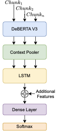
We propose an architecture based on the multilingual DeBERTa V3
model4 and a LSTM. In detail, first, a collection of chunks, from a
document, are passed through DeBERTa V3 to get their contextual
embeddings. Then, the first token of each embedding, i.e. the [CLS]
token, is passed through a dense layer and a GELU activation, to get a
context pool.5 After that, the collection of context pools are fed
into the LSTM. If available, additional features will be concatenated to
the final state of the LSTM. The final state will be fed then to a dense
layer and a Softmax activation for determining the class of the
document. In Figure
1, we present the architecture.
/>
Proposed architecture of the classifier.
As indicated in Section 3, rather than feeding a full document,
either as whole or split into small chunks, to the neural network, we
decided to randomly sample chunks. Therefore, we explored three sample
sizes, 20, 48 and 62. The sizes 20 and 62 were selected according to the
paragraphs’ quartiles of the corpus (see
Table [table:corpus]); the size 48 was
randomly chosen.6
To create the chunks, we split the documents into paragraphs7. Then,
each paragraph is tokenized and encoded with DeBERTa V3 tokenizer. If
the generated chunk surpasses 128 tokens, they are sub-split with an
overlapping stride of 16 tokens. The sampling is done over all the
document’s encoded chunks, and they are fed into the neural network
following the document’s order.
Besides, we explored 3 types of document length representations as
additional features8: number of characters ($`n_c`$), number of
paragraphs ($`n_p`$), and approximate number of pages
($`a_{pp} = n_c / 1,800`$)9. To keep these features in a close range
of values, all of them were represented using the natural logarithm.
In Table [tab:hyperparams], we present the
hyperparameters used for training the classifier. Moreover, it should be
noted that during the training process, the sampling process is done at
the beginning of each epoch. In other words, in each epoch, we feed the
neural network a collection of documents that has different chunks. The
goal was to make more robust the training of the document classifier by
providing different portions of text that could occur in a legal
document.
Data
We use a proprietary multilingual legal corpus related to the domain of
legal arbitration and covering 25 languages10.
All the documents were manually classified by legal experts into 18
classes throughout multiple years. In this work, we divided this corpus
into 3 sets, train (80%), dev (10%), and test (10%); all the data is
represented using JSON line files (JSONL). In
Table [table:corpus], we present the corpus’
statistics.
It should be seen that the approximate median number of pages of all the
corpus is 7.3. As well, that the longest documents in the corpus are
those belonging to the class Expert opinion (the median is 38.8
pages), while the shortest ones are those belonging to the class Other
(the median is 1 page). These figures were calculated by diving the
median number of characters by 1,800 (number of characters in a standard
page).
Deployment
Since the goal of the classifier is to be part of a larger project that
will be used along other tools, such as an OCR, and a metadata
extractor, we decided to deploy it within a processing pipeline.
Specifically, we used Temporal, an open-source orchestrator that allow
us creating robust and scalable workflows, in a simple way. Where we
focus only on the business logic, rather than coding as well, aspects
such as distribution of tasks, queue systems and state capture. Thus, in
this paper, we present the current workflow created in Temporal and its
deployment. However, it should be indicated that the described pipeline
will change in the near future, since we will add other components that
currently are being implemented.
Temporal uses 4 basic elements: Activities (a task or collection of
simple tasks), Workflows (a collection of Activities), Queues (a
waiting list of inputs for Activities and Workflows), and Workers (a
deployment instance that runs specific Activities and/or Workflows and
that listens a specific Queue). Moreover, each Activity and Workflow
process only one input at the time, but multiple Activities and
Workflows can be run at the same time. This can be done either by
configuring the Workers limits or by deploying more Workers.
All the input and outputs from/for a user (either a human or another
system) are communicated using Temporal’s client. This client can call a
specific workflow to run, with its respective input, and can either
return an ID (to ask later for the status), or wait for the workflow to
finish and return its output.
Pipeline
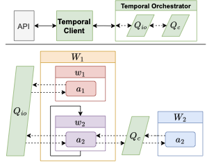
Our pipeline, at the current state, is composed of three Activities. The
first one, $`a_1`$, for a given directory, it finds all the JSON files
and produce a list of path files. The second one, $`a_2`$, it reads a
JSON file and validates it. The third one, $`a_3`$, process the JSON
file to create the input of the neural network and calls the neural
network to infer the class.11 Furthermore, this last Activity listens
to its unique Queue, $`Q_c`$, which is dedicated for documents ready to
be classified, rather than the Queue $`Q_{io}`$, which is for
input-output processing.
These Activities are split into two Workflows. The first Workflow,
$`w_1`$, calls $`a_2`$ and $`a_3`$; moreover, it creates batches of 10
documents to process. When a batch has been finished, if there are more
documents to process, it will create a new Workflow instance12. The
second Workflow $`w_2`$ calls Activity $`a_1`$ and Workflow $`w_1`$.
Finally, we have designed two Workers. The Worker $`W_1`$ is charged of
sending data to the Queue $`Q_{io}`$, and it manages, $`a_1`$ and
$`a_2`$, plus $`w_2`$ and part of $`w_1`$. The Worker $`W_2`$, connects
only to the Queue $`Q_c`$, which means that it only runs $`a_3`$. We can
have as many instances of each worker, and all of them will be
orchestrated by Temporal automatically. An API, deployed independently,
sends the input to process to Temporal. In
Figure 2, we have a diagram of
Temporal’s pipeline architecture.
/>
Temporal’s pipeline architecture. Dashed lines are indirect
communication managed by Temporal.
Results and Discussion
Sampling
Additional
Dev Weighted
Test Weighted
F-score Distribution
size
Features
F-score
Min
Q1
Q2
Q3
Max
48
npncapp
0.896
0.883
0.887
0.891
0.893
0.896
48
nc
0.896
0.882
0.888
0.891
0.893
0.897
62
app
0.894
0.886
0.890
0.893
0.895
0.886
62
-
0.892
0.891
0.895
0.898
0.900
0.904
62
np
0.891
0.875
0.882
0.886
0.887
0.890
20
-
0.869
0.860
0.867
0.871
0.872
0.887
We present, in Table [table:results], the results of the
top five models according to their weighted F-score over the dev set
calculated during their training.13 As well, we present the result of
the smallest sampling explored. It should be noted that the results,
regarding the test set
(Table [table:results]), were calculated
over 30 runs. The reason is that since we do at runtime (either training
or inference) a sampling of the documents’ paragraphs, each run will
generate a different weighted F-score. Thus, in this way, we can have a
better idea of the actual performance distribution for each model.
In Table [table:results], we can observe that,
in general, the models perform within a respectable range of values over
the test set, and no great variations are found. Moreover, there is no
big difference between the obtained weighted F-score on the dev set and
the median ($`Q_2`$) obtained on the test set. This means that our
approach of changing each epoch the chunks sent to the neural network
made ours models robust. However, the best weighted F-score in the dev
set did not reflect the best weighted F-score in the test set, although
this can be seen as problematic, this was expected, since during the
training we only run once per epoch the evaluation on the dev set.14
Interestingly, we can also notice in
Table [table:results], that even as few as
20 chunks can be useful for classifying documents, although with a
lesser performance, but still good enough for many tasks.
We present, in
Table [table:corpus_results], the
median F-scores obtained per each class in the test set over 30
runs15 regarding the best models found according to the dev and test
sets. As we can see in
Table [table:corpus_results], most
of the median F-scores are greater than 0.800, few are the exceptions,
such as Pleadings, Notice of intent, and Settlement agreement.
These last two classes of documents were some of the less frequent
documents in the training corpus.
We want to highlight, that we decided to include the additional features
because during the first experiments we were having issues differencing
two classes, Notice of intent and Notice of Arbitration. Both are
similar in structure, but according to our legal experts, the former
tend to be shorter than the latter. Although, this is not supported
according to the corpus’ statistics
(Table [table:corpus]), we considered that
nevertheless, the additional features could improve in general the
classification. Nonetheless, the addition or not of additional features
did not improve the classification of Notice of intent, which was the
class that was the most incorrectly misclassified of all the dataset.
While we consider that, maybe it is because Notice of intent is one of
the less frequent documents in the corpus, we ask ourselves as well
whether the issue comes as well from annotation errors, which might also
explain the length disagreement between the facts and the legal
knowledge of our team.
Furthermore, it is interesting to notice, that there is not a clear
relationship between low score, few documents and/or document length
from comparing Table [table:corpus] and
Table [table:corpus_results]. For
instance, Pleadings is a frequent class, but it had low performance.
The reason is that some Notice of request and Other requests are
sometimes considered as Pleadings. As well, in occasions Expert
opinions were misclassified as Witness statements, regardless of
whether we used the additional features and the fact that the former
tend to be the longest documents in the corpus. Something similar
happens between Settlement agreement and Contracts, where the latter
is sometimes the class predicted for the former documents, despite their
difference in length according to
Table [table:corpus].
Deployment analysis
With respect to the deployment using Temporal, we consider it a useful
and interesting tools for creating pipelines. For instance, it took us
around 2 hours to develop a functional pipeline locally16, and less
than a week having a much more robust pipeline that we could deploy in
our servers. As well, we really focused more on what we want the
pipeline to do, rather than focusing on how to orchestrate asynchronous
tasks, workers, queues, etc. For instance, it was very simple to
indicate that if the reading or validation of a file was unsuccessful
(e.g., does not exist or has the wrong format), the Activity should not
be retried again, without failing the whole process (see
Figure 3). But, if a Worker was down or
stopped giving signals of being alive, the failed Activities should be
retried $`n`$ times. Also, it is very simple to scale horizontally, we
just need to deploy another Worker, and Temporal will manage the rest,
e.g. sending to the Worker Activities that were waiting in the queue.
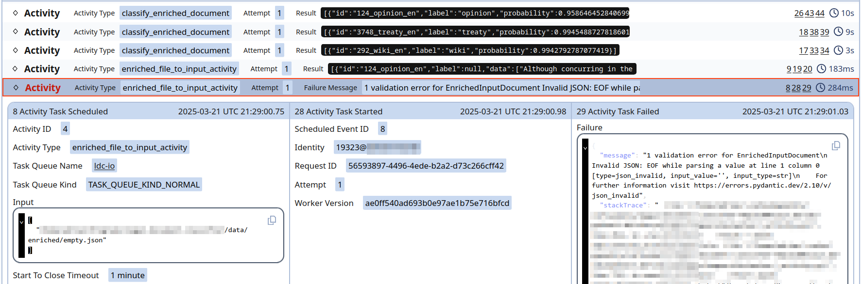
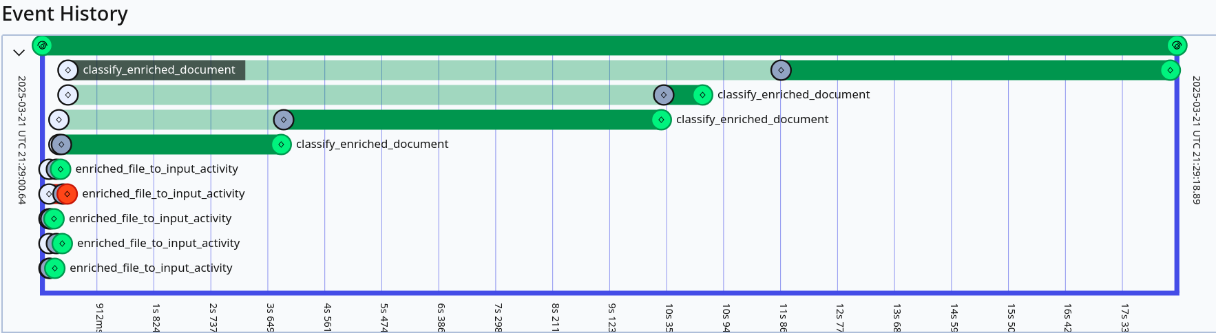
Event history as a diagram. The first circle indicates when
the task was received in the queue; the middle one is when it started to
run; the last one is when it ended. The fourth Activity,
enriched_file_to_input_activity, is red because it
failed.Event history as a collection of payloads. We can observe
the failed activity and the stack trace.Temporal’s event history. Despite errors in the workflow,
the pipeline continued until completed.
In Temporal’s interface, we can see the workflows’ event history
(Figure 3). For example, we can see how
long a Workflow/Activity took to start/finish, by which worker it was
done, which were the errors, and how many times were retried.17
Furthermore, encrypting and decrypting Temporal’s payloads (messages
send between Activities, Workflows and Workers), was extremely easy. The
only issue we had not expected about Temporal’s payloads, was their
limited size. In other words, Temporal communication between workflows
and activities are done using gRPC18 payloads, and these are
limited in size: 2MB for requests and 4MB for event history.19 Thus,
we had to change how and how many documents we processed. In other
words, we decided to split the list of documents to process in batches
of size 10; this splitting is done within Temporal’s logic, thus, for
the user there is no further task to be done.
We present, in
Table [table:inference_time], the
time needed for running 30 pipelines using Temporal for predicting 100
documents. The 100 documents were randomly sampled each run from the
test set; the goal was to explore the functioning of the pipeline over
different types of documents, and in consequence different combinations
of lengths. As well, to explore whether a batch of 10 documents was a
good fit for Temporal’s payloads.
It should be noted that the results presented in
Table [table:inference_time] were
done using a server that only has CPUs, and only one worker of each type
($`W_1`$ and $`W_2`$) was deployed. As well, the inference time
comprises the reading and validation of the documents; in other words,
it evaluated the full pipeline.
We can observe, in
Table [table:inference_time], that
the median time to process 100 documents is 498.080 seconds
($`\sim`$4.98 seconds per file). While it might not be bad for a
CPU processing (see for other comparisons), it is certainly far from the
median (calculated over more than 300 runs) of 68.002 seconds that an
NVIDIA A100 took for predicting the full test set (1,229 documents).
Conclusions and Future Work
Automatizing the classification of legal documents, while necessary for
simplifying the tasks of lawyers, can be challenging. This is due to the
characteristics of legal documents, such as specialized vocabulary and
length.
In this work, we introduced how Jus Mundi solved an internal need by
exploring the following hypothesis it is possible to classify (long)
legal documents using small and randomly-selected portions of text.
This hypothesis was defined due to internal constraints, but also from
observations and results that other researchers in the state-of-the-art
have produced. Therefore, we presented the architecture and methodology
for creating a classifier for legal documents that uses up to 48 random
chunks of maximum 128 tokens. Furthermore, in this work, we explained
how we deployed the classifier in our servers using Temporal, an
open-source durable execution solution, for creating pipelines that
could be used by our tools and services.
The results obtained, showed that it is possible to classify documents
correctly using random short chunks. Specifically, our models can reach
a median weighted F-score of 0.898 and a median speed of
$`\sim`$4.98 seconds per file on a CPU server. As well, we
noticed that the use of Temporal for creating pipelines can simplify
their design, coding and deployment.
In the future, we want to convert our current PyTorch model into a
ONNX20 one, using the ONNX Runtime21. The goal is to improve
the inference by optimizing the model, even exploring its quantization.
As well, we want to compress payloads using Zstandard22, for
increasing Temporal’s batch size. And at the same time, we need to
improve the batching logic used in the neural network when deployed
using Temporal, since right now it only processes one document at the
time.
Finally, we want to analyze deeper the misclassified documents with our
legal team, in order to better understand what could be the reasons for
some of the errors presented in this work. And to analyze whether the
language of a document plays a role regarding the classification
problems of certain documents and how it affects the global performance
of our legal document classifier.
Ethical considerations
All the documents used for the development of the classifiers were
obtained fairly. In other words, these were either written by our legal
team or obtained from public sources, collaborations and through
partnerships that indicated that we could use their documents for
training machine learning models. As well, documents with sensitive
information were previously anonymized, by experts, and we, the
developers of the classifier, did not have access to the original
documents.
Acknowledgments
This work was possible due to the granted access of IDRIS (Institut du
Développement et des Ressources en Informatique Scientifique)
High-performance computing resources under the allocation
2024-AD011012667R3 made by GENCI (Grand Équipement National de Calcul
Intensif).
The copyright of this content belongs to the respective researchers. We deeply appreciate their hard work and contribution to the advancement of human civilization.
Although we tried to explore, larger contexts, up to samples of
160 chunks, their training was complex. Those that we partially
managed to train (80 and 120), were slower, used more memory, and
were not better than those presented here. ↩︎
Our data was originally in HTML, thus we used tags such as <p>
(paragraph) and <li> (listing) for splitting the texts. ↩︎
According to our legal experts, the document length could be a
good discriminator of the classes. ↩︎
We do not have the original number of pages for all documents,
this is why it is approximated. ↩︎
Certain documents have versions in multiple languages. For those
cases, we only considered one language, giving priority to those
different from English, French, Spanish and Portuguese, since these
were the most frequent ones: 9,378, 1,602, 998, and 255 documents
respectively. ↩︎
We did not use a different Activity for the creation of the
neural network input, since it would have been too expensive to do.
In other words, we would need to convert a document (JSON) into
Numpy arrays (by tokenizing and encoding it) and then into a new
JSON. Then this new JSON would have to be parsed to convert it into
a Torch tensor. ↩︎
This is to avoid an explosion of the history event. See
[https://docs.temporal.io/develop/python/continue-as-new](Continue as new). ↩︎
We use the weighted F-score since the corpus is imbalance. Some
classes in the dev and test set have as few as 14 documents. ↩︎
In the future, we will add the possibility of running multiple
evaluations during the training, to be sure to select the actual
best model. ↩︎