Conducting machine learning on streaming time series data introduces additional challenges beyond those encountered with machine learning on static data. These challenges include overfitting, feature engineering, model evaluation, data pipeline engineering. These issues are compounded by the dynamic nature of streaming data.

In the following we list several problems in time-series machine learning and how DataFlow solves these problems.

Prototype vs Production

Data scientists typically operate under the assumption that all data is readily available in a well-organized data frame format. Consequently, they often develop a prototype based on assumptions about the temporal alignment of the data. This prototype is then transformed into a production system by rewriting the model in a more sophisticated and precise framework. This process may involve using different programming languages or even having different teams handle the translation. However, this approach can lead to significant issues:

• Converting the prototype in production requires time and effort

• The translation process may reveal bugs in the prototype.

• Assumptions made during the prototype phase might not align with real-world conditions.

• Discrepancies between the two model can result in additional work to implement and maintain two separate models for comparison.

DataFlow addresses this issue by modeling systems as directed acyclic graphs (DAGs), which naturally align with the dataflow and reactive models commonly used in real-time systems. Each node within the graph consists of procedural statements, similar to how a data scientist would design a non-streaming system.

DataFlow enables the execution of a model in both batch and streaming modes without requiring any modifications to the model code. In batch Mode, the graph can be executed by processing data all at once or in segments, suitable for historical or batch processing. In streaming mode, the graph can also be executed as data is presented to the model, supporting real-time data processing.

Frequency of Model Operation

The required frequency of a model’s operation often becomes clear only after deployment. Adjustments may be necessary to balance time and memory requirements with latency and throughput, which require changing the production system implementation, with further waste of engineering effort.

DataFlow enables the same model description to operate at various frequencies by simply adjusting the size of the computation tile. This flexibility eliminates the need for any model modifications and allows models to be always run at the optimal frequency requested by the application.

Non-stationarity time series

While the assumption of stationarity is useful, it typically only strictly holds in theoretical fields such as physics and mathematics. In practical, real-world applications, this assumption is rarely valid. Data scientists often refer to data drift as an anomaly to explain poor performance on out-of-sample data. However, in reality, data drift is the standard rather than the exception.

All DataFlow components, including the data store, compute engine, and deployment, are designed to natively handle time series processing. Each time series can be either univariate or multivariate (such as panel data) and is represented in a data frame format. DataFlow addresses non-stationarity by enabling models to learn and predict continuously over time. This is achieved using a specified look-back period or a weighting scheme for samples. These parameters are treated as hyperparameters of the system, which can be tuned like any other hyperparameters.

Non-causal Bugs

A common and challenging problem occurs when data scientists make incorrect assumptions about data timestamps. This issue is often called “future peeking” because the model inadvertently uses future information. A model is developed, validated, and fine-tuned based on these incorrect assumptions, which are only identified as errors after the system is deployed in production. This happens because the data scientist lacks an early, independent evaluation to identify the presence of non-causality.

Figure 1 illustrates a concrete example of this bug pattern.

# Uses tomorrow's price!
df['signal'] = df['price'].shift(-1)

# At time t, this accesses
# price at time t+1

# Uses yesterday's price
df['signal'] = df['price'].shift(1)

# At time t, this accesses
# price at time t-1

DataFlow offers precise time management. Each component automatically monitors the time at which data becomes available at both its input and output. This feature helps in easily identifying future peeking bugs, where a system improperly uses data from the future, violating causality. DataFlow ensures consistent model execution regardless of how data is fed, provided the model adheres to strict causality. Testing frameworks are available to compare batch and streaming results, enabling early detection of any causality issues during the development process.

Accurate Historical Simulation

Implementing an accurate simulation of a system that processes time-series data to evaluate its performance can be quite challenging. Ideally, the simulation should replicate the exact setup that the system will use in production. For example, to compute the profit-and-loss curve of a trading model based on historical data, trades should be computed using only the information available at those moments and should be simulated at the precise times they would have occurred.

However, data scientists often create their own simplified simulation frameworks alongside their prototypes. The various learning, validation, and testing styles (such as in-sample-only and cross-validation) combined with walkthrough simulations (like rolling window and expanding window) result in a complex matrix of functionalities that need to be implemented, unit tested, and maintained.

DataFlow integrates these components once and for all into the framework, to streamline the process and allow to running detailed simulation in the design phase. DataFlow supports many different learning styles from different types of runners (e.g., in-sample-only, in-sample vs out-of-sample, rolling learning, cross-validation) together with

Debugging production systems

The importance of comparing production systems with simulations is highlighted by the following typical activities:

• Quality Assessment: To evaluate the assumptions made during the design phase, ensuring that models perform consistently with both real-time and historical data. This process is often called “reconciliation between research and production models.”

• Model Evaluation: To assess how models respond to changes in real-world conditions. For example, understanding the impact of data arriving one second later than expected.

• Debugging: Production systems occasionally fail and require offline debugging. To troubleshoot production models by extracting values at internal nodes to identify and resolve failures.

In many engineering setups, there is no systematic approach to conducting these analyses. As a result, data scientists and engineers often rely on cumbersome and time-consuming ad-hoc methods to compare models.

DataFlow solves the problem of observability and debuggability of models by easily allowing to capture and replay the execution of any subset of nodes. In this way, it is possible to easily observe and debug the behavior of a complex system. This comes naturally from the fact that research and production systems are the same, from the accurate timing semantic of the simulation kernel.

Model performance

Performance of research and production systems need to be tuned to accomplish various tradeoff (e.g., fit in memory, maximize throughput, minimize latency).

DataFlow addresses the model performance and its tradeoffs with several techniques including:

• Tiling. DataFlow’s framework allows streaming data with different tiling styles (e.g., across time, across features, and both), to minimize the amount of working memory needed for a given computation, increasing the chances of caching computation.

• Incremental computation and caching. Because the dependencies between nodes are explicitly tracked by DataFlow, only nodes that see a change of inputs or in the implementation code need to be recomputed, while the redundant computation can be automatically cached.

• Maximum parallelism. Because the computation is expressed as a DAG, the DataFlow execution scheduler can extract the maximum amount of parallelism and execute multiple nodes in parallel in a distributed fashion, minimizing latency and maximizing throughput of a computation.

• Automatic vectorization. DataFlow nodes can use all native vectorization approaches available in numpy and Pandas.

Performing parameters analyis

Tracking and sweeping parameter is a common challenge in machine learning projects:

• During the research phase, data scientists perform numerous simulations to explore the parameter space. It is crucial to systematically specify and track these parameter sweeps

• Once the model is finalized, the model parameters must be fixed and these parameters should be deployed alongside the production system

In a DataFlow system it is easy to generate variations of DAGs using a declarative approach to facilitate the adjustment of multiple parameters to comprehensively explore the design space.

• Each parameter is governed by a specific value within a configuration. This implies that the configuration space is equivalent to the space of DataFlow systems: each configuration uniquely defines a DataFlow system, and each DataFlow system is completely described by a configuration

• A configuration is organized as a nested dictionary, reflecting the structure of the Directed Acyclic Graph (DAG). This organization enables straightforward navigation through its structure

Challenges in time series MLOps

The complexity of Machine Learning Operations (MLOps) arises from managing the full lifecycle of ML models in production. This includes not just training and evaluation, but also deployment, monitoring, and governance.

DataFlow provides solutions to MLOps challenges fully integrated in the framework.

• Model Serialization. Once a Directed Acyclic Graph (DAG) is fitted, it can be saved to disk. This serialized model can later be loaded and used for making predictions in a production environment

• Deployment and Monitoring. Any DataFlow system is deployable as a Docker container. This includes the development system, which also operates within a Docker container. This setup facilitates the development and testing of systems on both cloud platforms (such as AWS) and local machines. Airflow is natively utilized for scheduling and monitoring long-running DataFlow systems.

Execution Engine

Graph computation

DataFlow model

A DataFlow model (aka DAG) is a direct acyclic graph composed of DataFlow nodes

It allows one to connect, query the structure, …

Running a method on a DAG means running that method on all its nodes in topological order, propagating values through the DAG nodes.

TODO(Paul, Samarth): Add picture.

DagConfig

A Dag can be built by assembling Nodes using a function representing the connectivity of the nodes and parameters contained in a Config (e.g., through a call to a builder DagBuilder.get_dag(config)).

A DagConfig is hierarchical and contains one subconfig per DAG node. It should only include Dag node configuration parameters, and not information about Dag connectivity, which is specified in the Dag builder part. A Dag can be built by assembling Nodes using a function representing the connectivity of the nodes and parameters contained in a Config (e.g., through a call to a builder DagBuilder.get_dag(config)).

A DagConfig is hierarchical and contains one subconfig per DAG node. It should only include Dag node configuration parameters, and not information about Dag connectivity, which is specified in the Dag builder part.

Graph execution

Simulation kernel

A computation graph is a directed graph where nodes represent operations or variables, and edges represent dependencies between these operations.

For example, in a computation graph for a mathematical expression, nodes would represent operations like addition or multiplication, while edges would indicate the order (and grouping) of operations.

The DataFlow simulation kernel schedules nodes according to their dependencies.

Simulation kernel details

The most general case of simulation consists of multiple nested loops:

1. Multiple DAG computation. The general workload contains multiple DAG computations, each one inferred through a Config belonging to a list of Configs describing the entire workload to execute.

   • In this set-up each DAG computation is independent, although some pieces of computations can be common across the workload. DataFlow will compute and then cache the common computations automatically as part of the framework execution

2. Learning pattern. For each DAG computation, multiple train/predict loops represent different machine learning patterns (e.g., in-sample vs out-of-sample, cross-validation, rolling window)

   • This loop accommodates the need for nodes with state to be driven to learn parameters and hyperparameters and then use the learned state to predict on unseen data (i.e., out-of-sample)

3. Temporal tiling. Each DAG computation runs over a tile representing an interval of time

   • As explained in section XYZ, DataFlow partition the time dimension in multiple tiles

   • Temporal tiles might overlap to accommodate the amount of memory needed by each node (see XYZ), thus each timestamp will be covered by at least one tile. In the case of DAG nodes with no memory, then time is partitioned in non-overlapping tiles.

   • The tiling pattern over time does not affect the result as long as the system is properly designed (see XYZ)

4. Spatial tiling. Each temporal slice can be computed in terms of multiple sections across the horizontal dimension of the dataframe inputs, as explained in section XYZ.

   • This is constrained by nodes that compute features cross-sectionally, which require the entire space slice to be computed at once

5. Single DAG computation. Finally a topological sorting based on the specific DAG connectivity is performed in order to execute nodes in the proper order. Each node executes over temporal and spatial tiles.

Figure 2 illustrates the nested structure of these simulation loops.

Note that it is possible to represent all the computations from the above loops in a single “scheduling graph” and use this graph to schedule executions in a global fashion.

Parallelization across CPUs comes naturally from the previous approach, since computations that are independent in the scheduling graph can be executed in parallel, as described in Section XYZ.

Incremental and cached computation is built-in in the scheduling algorithm since it’s possible to memoize the output by checking for a hash of all the inputs and of the code in each node, as described in Section XYZ.

Even though each single DAG computation is required to have no loops, a System (see XYZ) can have components introducing loops in the computation (e.g., a Portfolio component in a trading system, where a DAG computes forecasts which are acted upon based on the available funds). In this case, the simulation kernel needs to enforce dependencies in the time dimension.

Node ordering for execution

TODO(gp, Paul): Extend this to the multiple loop.

Topological sorting is a linear ordering of the vertices of a directed graph such that for every directed edge from vertex u to vertex v, u comes before v in the ordering. This sorting is only possible if the graph has no directed cycles, i.e., it must be a Directed Acyclic Graph (DAG).

def topological_sort(graph):
  visited = set()
  post_order = []

  def dfs(node):
      if node in visited:
          return
      visited.add(node)
      for neighbor in graph.get(node, []):
          dfs(neighbor)
      post_order.append(node)

  for node in graph:
      dfs(node)

  return post_order[::-1]  # Reverse the post-order to get the topological order

Heuristics for splitting computational steps into nodes

There are degrees of freedom in splitting the work between various nodes of a graph E.g., the same DataFlow computation can be described with several nodes or with a single node containing all the code

The trade-off is often between several metrics:

• Observability

  • More nodes make it easier to:

    • observe and debug intermediate the result of complex computation

    • profile graph executions to understand performance bottlenecks

• latency/throughput

  • More nodes:

    • allows for better caching of computation

    • allows for smaller incremental computation when only one part of the inputs change

    • prevents optimizations performed across nodes

    • incurs in more simulation kernel overhead for scheduling

    • allows more parallelism between nodes being extracted and exploited

• memory consumption

  • More nodes:

    • allows one to partition the computation in smaller chunks requiring less working memory

A possible heuristic is to start with smaller nodes, where each node has a clear function, and then merge nodes if this is shown to improve performance

DataFlow System

Motivation

While DataFlow requires that a DAG should not have cycles, general computing systems might need to reuse the state from computation performed on past data. E.g., in a trading system, there is often a Forecast component that can be modeled as a DAG with no cycles and a Portfolio object that uses the forecasts to compute the desired allocation of capital across different positions based on the previous positions.

DataFlow supports this need by assembling multiple DAGs into a complete System that allows cycles.

The assumption is that DAGs are computationally expensive, while other components mainly execute light procedural computation that requires interaction with external objects such as databases, filesystems, sockets.

TODO(gp): Add picture

TODO(gp): Explain that System are derived from other Python objects.

Timing semantic and clocks

Time semantics

DataFlow components can execute in real-time or simulated mode, with different approaches for representing the passage of time. The framework supports multiple temporal execution modes designed to prevent future peeking while maintaining consistency between simulation and production environments.

Clock types

The framework defines three distinct clock implementations:

1. Static clock: A clock that remains constant during system execution. Future peeking is technically permissible with this clock type.

2. Replayed clock: A clock that advances through historical time, either synchronized with wall-clock time or driven by computational events. The clock can be positioned in either past or future relative to actual time, but future peeking is prohibited to maintain simulation fidelity.

3. Real clock: The wall-clock time, where data becomes available as generated by external systems. Future peeking is inherently impossible.

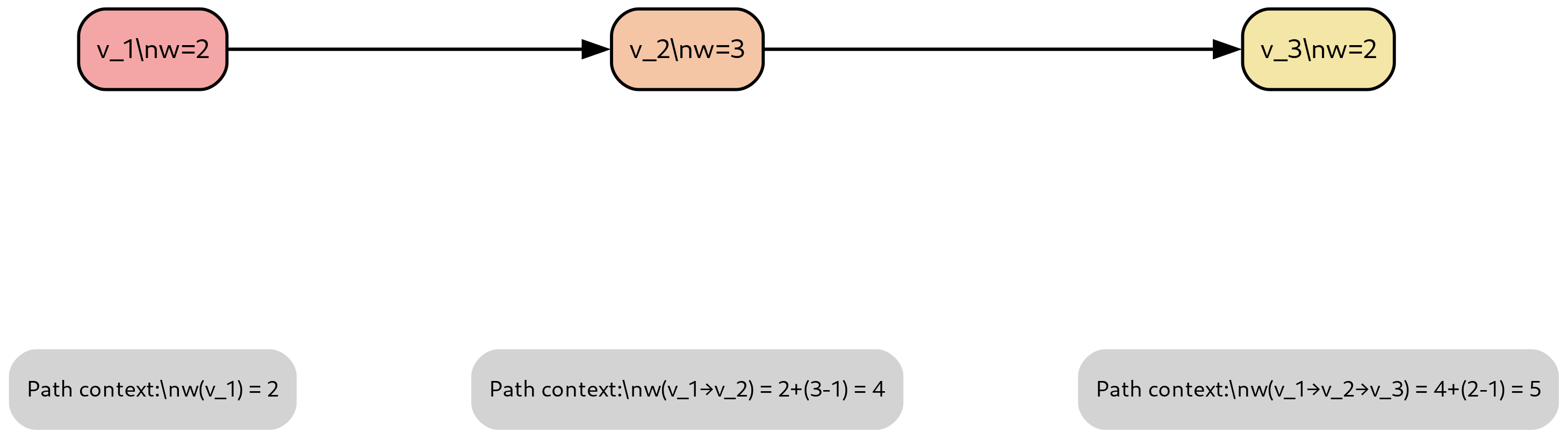
Knowledge time

Knowledge time represents the timestamp when data becomes available to the system, either through download or computation. Each data row is annotated with its corresponding knowledge time. The framework enforces that data with knowledge time exceeding the current clock time remains inaccessible, preventing inadvertent future peeking.

Timed and non-timed simulation

Timed simulation. In timed simulation (also referred to as historical, vectorized, or batch simulation), data is provided with an advancing clock that reports the current timestamp. The system enforces that only data with knowledge time less than or equal to the current timestamp is observable, thus preventing future peeking. This mode typically employs either a replayed clock or static clock depending on the specific use case.

Non-timed simulation. In non-timed simulation (also referred to as event-based or reactive simulation), the clock type is static. The wall-clock time corresponds to a timestamp equal to or greater than the latest knowledge time in the dataset. Consequently, all data in the dataframe becomes immediately available since each row has a knowledge time less than or equal to the wall-clock time. In this mode, data for the entire period of interest is provided as a single dataframe.

For example, consider a system generating predictions every 5 minutes. In non-timed simulation, all input data are equally spaced on a 5-minute grid and indexed by knowledge time:

df["c"] = (df["a"] + df["b"]).shift(1)

Real-time execution

In real-time execution, the clock type is a real clock. For a system predicting every 5 minutes, one forecast is generated every 5 minutes of wall-clock time, with data arriving incrementally rather than in bulk.

Replayed simulation

In replayed simulation, data is provided in the same format and timing as in real-time execution, but the clock type is a replayed clock. This allows the system to simulate real-time behavior while processing historical data, facilitating testing and validation of production systems.

Synchronous and asynchronous execution modes

Asynchronous mode. In asynchronous mode, multiple system components execute concurrently. For example, the DAG may compute while orders are transmitted to the market and other components await responses. The implementation utilizes Python’s asyncio framework. While true asynchronous execution typically requires multiple CPUs, under certain conditions (e.g., when I/O operations overlap with computation), a single CPU can effectively simulate asynchronous behavior.

Synchronous mode. In synchronous mode, components execute sequentially. For instance, the DAG completes its computation, then passes the resulting dataframe to the Order Management System (OMS), which subsequently executes orders and updates the portfolio.

The framework supports simulating the same system in either synchronous or asynchronous mode. Synchronous execution follows a sequential pattern: the DAG computes, passes data to the OMS, which then executes orders and updates the portfolio. Asynchronous execution creates persistently active objects that coordinate through mutual blocking mechanisms.

Vectorization

Vectorization

Vectorization is a technique for enhancing the performance of computations by simultaneously processing multiple data elements with a single instruction, leveraging the capabilities of modern processors (e.g., SIMD (Single Instruction, Multiple Data) units).

Vectorization in DataFlow

Given the DataFlow format, where features are organized in a hierarchical structure, DataFlow allows one to apply an operation to be applied across the cross-section of a dataframe. In this way DataFlow exploits Pandas and NumPy data manipulation and numerical computing capabilities, which are in turns built on top of low-level libraries written in languages like C and Fortran. These languages provide efficient implementations of vectorized operations, thus bypassing the slower execution speed of Python loops.

Example of vectorized node in DataFlow

TODO

Incremental, cached, and parallel execution

DataFlow and functional programming

The DataFlow computation model shares many similarity with functional programming:

• Data immutability: data in dataframe columns is typically added or replaced. A node in a DataFlow graph cannot alter data in the nodes earlier in the graph.

• Pure functions: the output of a node depends only on its input values and it does not cause observable side effects, such as modifying a global state or changing the value of its inputs

• Lack of global state: nodes do not rely on data outside their scope, especially global state

Incremental computation

Only parts of a compute graph that see a change of inputs need to be recomputed.

Incremental computation is an approach where the result of a computation is updated in response to changes in its inputs, rather than recalculating everything from scratch

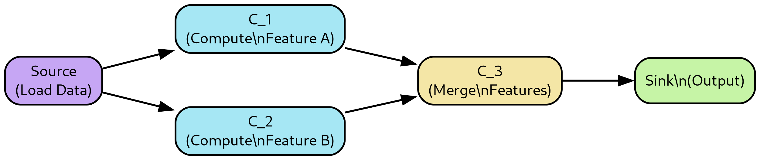
Caching

Because of the “functional” style (no side effects) of data flow, the output of a node is determinstic and function only of its inputs and code.

Thus the computation can be cached across runs. E.g., if many DAG simulations share the first part of simulation, then that part will be automatically cached and reused, without needing to be recomputed multiple times.

Figure 3 shows the caching algorithm used by DataFlow.

Parallel execution

Parallel and distributed execution in DataFlow is supported at two different levels:

• Across runs: given a list of Config, each describing a different system, each simulation can be in parallel because they are completely independent.

• Intra runs: each DataFlow graph can be run exploiting the fact that nodes

In the current implementation for intra-run parallelism Kaizen flow relies on Dask For across-run parallelism DataFlow relies on joblib or Dask

Dask extends the capabilities of the Python ecosystem by providing an efficient way to perform parallel and distributed computing.

Dask supports various forms of parallelism, including multi-threading, multi-processing, and distributed computing. This allows it to leverage multiple cores and machines for computation.

When working in a distributed environment, Dask distributes data and computation across multiple nodes in a cluster, managing communication and synchronization between nodes. It also provides resilience by re-computing lost data if a node fails.

Train and predict

A DAG computation may undergo multiple evaluation phases (also referred to as methods) to accommodate different experimental designs and validation strategies.

Evaluation phases

The framework supports several distinct phases:

• Initialization phase: Performs computations necessary to establish an initial state, such as loading previously learned model parameters.

• Fit phase: Learns the state of stateful nodes using training data.

• Validate phase: Tunes hyperparameters of the system using a validation set. Examples include determining the optimal number of epochs or layers in a neural network, or the time constant of a smoothing parameter.

• Predict phase: Applies the learned state of each node to generate predictions on unseen data.

• Load state: Retrieves previously learned state of stateful DAG nodes, such as trained model weights.

• Save state: Persists the learned state of a DAG following a fit phase, enabling subsequent deployment to production environments.

• Save results: Stores artifacts generated during model execution, such as predictions from a predict phase.

The simulation kernel schedules these phases according to the type of simulation and the dependency structure across DAG nodes. For instance, the initialization phase can load previously learned DAG state, enabling a subsequent predict phase without requiring a fit phase.

Experimental designs

In-sample evaluation

In-sample evaluation tests the model on the same dataset used for training. While this approach provides optimistic performance estimates, it serves as a useful baseline. The process consists of:

1. Feeding all data to the DAG in fit mode

2. Learning parameters for each stateful node

3. Running the DAG in predict mode on the training data

Train/test evaluation

Train/test evaluation (also known as in-sample/out-of-sample evaluation) partitions the data into disjoint training and test sets:

1. Split the data into training and test sets without temporal overlap

2. Feed training data to the DAG in fit mode

3. Learn parameters for each stateful node

4. Run the DAG in predict mode on the test data

Train/validate/test evaluation

This extends the train/test approach by introducing a validation set for hyperparameter tuning. The validation set enables selection of design parameters such as network architecture or regularization strength before final evaluation on the test set.

Cross-validation

Cross-validation provides robust model evaluation by partitioning the dataset into multiple subsets. For each partition:

1. Use one subset as the test set and remaining data as training set

2. Feed training data to the DAG in fit mode

3. Learn parameters for each stateful node

4. Run the DAG in predict mode on the test subset

Aggregate performance across all subsets to assess overall model quality. For time series data, this approach must respect temporal ordering to prevent future peeking.

Rolling train/test evaluation

Rolling evaluation is particularly suited for time series analysis. The approach sequentially partitions the dataset such that each test set immediately follows its corresponding training set in time:

1. Partition the dataset into sequential train and test sets

2. For each partition:

   • Use earlier data as the training set

   • Use immediately following data as the test set

   • Feed training data to the DAG in fit mode

   • Learn parameters for each stateful node

   • Run the DAG in predict mode on the test data

This method simulates realistic scenarios where the model is trained on historical data and tested on future observations, with the model continually updated as new data becomes available.

Stateful nodes

A DAG node is stateful if it uses data to learn parameters (e.g., linear regression coefficients, weights in a neural network, support vectors in a SVM) during the fit stage, that are then used in a successive predict stage.

The state is stored inside the implementation of the node.

The state of stateful DAG node varies during a single simulation.

The following example demonstrates a stateful node implementation:

class MovingAverageNode(Node):
    """
    Stateful node that learns optimal window size during fit phase
    and applies it during predict phase.
    """

    def __init__(self, nid: str, window_range: tuple = (5, 50)):
        """
        Args:
            nid: Unique node identifier
            window_range: Range of window sizes to search (min, max)
        """
        super().__init__(nid)
        self.window_range = window_range
        self.optimal_window = None  # Learned state

    def fit(self, df: pd.DataFrame) -> pd.DataFrame:
        """
        Learn optimal window size from training data using
        cross-validation on a holdout metric.
        """
        best_score = float('inf')
        best_window = self.window_range[0]

        # Search for optimal window size
        for window in range(*self.window_range):
            ma = df['price'].rolling(window=window).mean()
            # Evaluate on some metric (e.g., forecast error)
            score = self._evaluate_window(df, ma)
            if score < best_score:
                best_score = score
                best_window = window

        # Store learned state
        self.optimal_window = best_window
        return self._compute_ma(df, best_window)

    def predict(self, df: pd.DataFrame) -> pd.DataFrame:
        """
        Apply learned window size to new data.
        State must be set before calling predict.
        """
        assert self.optimal_window is not None, \
            "Must call fit() before predict()"
        return self._compute_ma(df, self.optimal_window)

    def _compute_ma(self, df: pd.DataFrame, window: int) -> pd.DataFrame:
        """Compute moving average with given window."""
        df_out = df.copy()
        df_out['ma'] = df['price'].rolling(window=window).mean()
        return df_out

    def _evaluate_window(self, df: pd.DataFrame,
                        ma: pd.Series) -> float:
        """Evaluate window size quality (implementation detail)."""
        # Example: mean squared error on next-step prediction
        return ((df['price'].shift(-1) - ma) ** 2).mean()

Stateless nodes

A DAG node is stateless if the output is not dependent on previous fit stages. In other words the output of the node is only function of the current inputs and of the node code, but not from inputs from previous tiles of inputs.

A stateless DAG node emits the same output independently from the current and previous fit vs predict phases.

A stateless DAG node has no state that needs to be stored across a simulation.

Loading and saving node state

Each stateful node provides mechanisms for persisting and retrieving its internal state on demand. The framework orchestrates the serialization and deserialization of entire DAG states to disk.

A stateless node returns an empty state when saving and raises an assertion error if presented with a non-empty state during loading.

The framework enables loading DAG state for subsequent analysis. For instance, one might examine how linear model weights evolve over time in a rolling window simulation.

Batch computation and tiled execution

DataFlow supports batch computation through tiled execution, which partitions computation across temporal and spatial dimensions. Tiled execution provides several advantages:

• Memory efficiency: Large-scale simulations that exceed available memory can be executed by processing data in manageable tiles.

• Incremental computation: Results can be computed progressively and cached, avoiding redundant calculations.

• Parallelization: Independent tiles can be processed concurrently across multiple compute resources.

Temporal tiling

Temporal tiling partitions the time dimension into intervals. Each tile represents a specific time period (e.g., a single day or month). Tiles may overlap to accommodate node memory requirements. For nodes without memory dependencies, time is partitioned into non-overlapping intervals.

Spatial tiling

Within each temporal slice, computation may be further divided across the horizontal dimension of dataframes. This approach is constrained by nodes that compute cross-sectional features, which require simultaneous access to the entire spatial slice.

DAG runner implementations

Different DagRunner implementations support various execution patterns:

• FitPredictDagRunner: Implements separate fit and predict phases for in-sample and out-of-sample evaluation.

• RollingFitPredictDagRunner: Supports rolling window evaluation with periodic retraining.

• RealTimeDagRunner: Executes nodes with real-time semantics, processing data as it arrives.

Backtesting and model evaluation

Backtesting provides a framework for evaluating model performance on historical data, supporting various levels of abstraction and fidelity to production environments.

Backtest execution modes

A backtest consists of code configured by a single Config object. The framework supports multiple execution modes:

• Batch mode: All data is available from the outset and processed in bulk, either as a single operation or partitioned into tiles. No clock advancement occurs during execution.

• Streaming mode: Data becomes available incrementally as a clock advances, simulating real-time operation. This mode is equivalent to processing tiles with temporal span matching the data arrival frequency.

Research flow

The research flow provides rapid model evaluation without portfolio management complexity. This mode excludes position tracking, order submission, and exchange interaction. Consequently, transaction costs and market microstructure effects are not reflected in performance metrics. The research flow proves valuable for assessing predictive power and conducting preliminary model comparison.

Tiled backtesting

Tiled backtesting extends the basic backtest concept by partitioning execution across multiple dimensions:

• Asset dimension: Each tile processes a subset of assets, potentially a single instrument, over the entire time period.

• Temporal dimension: Each tile processes all assets over a specific time interval (e.g., one day or month), closely resembling real-time system operation.

• Hybrid tiling: Arbitrary partitioning across both dimensions to optimize memory usage and computational efficiency.

The framework represents each tile as a Config object. Source nodes support tiling through Parquet and database backends, computation nodes handle tiling naturally through DataFlow’s streaming architecture, and sink nodes write results using Hive-partitioned Parquet format.

Configuration and reproducibility

The framework employs hierarchical Config objects to ensure reproducibility:

• DagConfig: Contains node-specific parameters, excluding connectivity information which is specified in the DagBuilder.

• SystemConfig: Encompasses the entire system specification, including market data configuration, execution parameters, and DAG configuration.

• BacktestConfig: Defines temporal boundaries, universe selection, trading frequency, and data lookback requirements.

Each configuration is serialized and stored alongside results, enabling precise reproduction of experiments.

Observability and debuggability

Running a DAG partially

DataFlow allows one to run nodes and DAGs in a notebook during design, analysis, and debugging phases, and in a Python script during simulation and production phases.

It is possible to run a DAG up to a certain node to iterate on its design and debug.

TODO: Add example

Replaying a DAG

Each DAG node can:

• capture the stream of data presented to it during either a simulation and real-time execution

• serialize the inputs and the outputs, together with the knowledge timestamps

• play back the outputs

DataFlow allows one to describe a cut in a DAG and capture the inputs and outputs at that interface. In this way it is possible to debug a DAG replacing all the components before a given cut with a synthetic one replaying the observed behavior together with the exact timing in terms of knowledge timestamps.

This allows one to easily:

• capture failures in production and replay them in simulation for debugging

• write unit tests using observed data traces

DataFlow allows each node to automatically save all the inputs and outputs to disk to allow replay and analysis of the behavior with high fidelity.