Deep Learning in Geotechnical Engineering A Critical Assessment of PINNs and Operator Learning
📝 Original Paper Info
- Title: Deep Learning in Geotechnical Engineering A Critical Assessment of PINNs and Operator Learning- ArXiv ID: 2512.24365
- Date: 2025-12-30
- Authors: Krishna Kumar
📝 Abstract
Deep learning methods -- physics-informed neural networks (PINNs), deep operator networks (DeepONet), and graph network simulators (GNS) -- are increasingly proposed for geotechnical problems. This paper tests these methods against traditional solvers on canonical problems: wave propagation and beam-foundation interaction. PINNs run 90,000 times slower than finite difference with larger errors. DeepONet requires thousands of training simulations and breaks even only after millions of evaluations. Multi-layer perceptrons fail catastrophically when extrapolating beyond training data -- the common case in geotechnical prediction. GNS shows promise for geometry-agnostic simulation but faces scaling limits and cannot capture path-dependent soil behavior. For inverse problems, automatic differentiation through traditional solvers recovers material parameters with sub-percent accuracy in seconds. We recommend: use automatic differentiation for inverse problems; apply site-based cross-validation to account for spatial autocorrelation; reserve neural networks for problems where traditional solvers are genuinely expensive and predictions remain within the training envelope. When a method is four orders of magnitude slower with less accuracy, it is not a viable replacement for proven solvers.💡 Summary & Analysis
**3 Key Contributions** 1. **Limitations of Machine Learning**: Shows that neural networks are optimized for past data and can fail in future predictions. 2. **Spatial Autocorrelation Issue**: Geotechnical data is spatially correlated, leading to overestimation of accuracy if random splits are used for testing. 3. **Alternative with Automatic Differentiation**: Proposes automatic differentiation as an effective alternative for inverse problems.Simple Explanation and Metaphors
- Importance of Comparison: Before believing machine learning is better than traditional methods, direct numerical comparison should be made. This is like testing a new kitchen gadget to see if it works properly before purchasing.
- Prediction Limitations: Machine learning models are optimized only for past data and can fail in future predictions. It’s akin to weather forecasting not being accurate just by knowing yesterday’s weather.
- Spatial Autocorrelation: Geotechnical data is spatially correlated, leading to overestimation of accuracy if random splits are used for testing. This is like predicting the weather using data from a single location when it varies across different neighborhoods.
Sci-Tube Style Script
- Beginner Level: To debunk the myth that machine learning is faster and more accurate than traditional methods, we compared them directly with numbers. What were the results?
- Intermediate Level: We showed that neural networks are optimized only for past data and can fail in future predictions. We also explained the spatial autocorrelation issue.
- Advanced Level: This paper analyzes the limitations of machine learning and proposes automatic differentiation as a solution.
📄 Full Paper Content (ArXiv Source)
Machine learning (ML) methods are increasingly proposed as replacements for traditional geotechnical analyses, promising instant predictions that bypass expensive solvers . Applications now common in geotechnical journals include physics-informed neural networks (PINNs) for wave propagation and deep operator networks (DeepONet) for foundation response. The promise is compelling: train a model once on past case histories, then predict instantly for new conditions. But should we believe this promise? More precisely, under what conditions does machine learning genuinely outperform the traditional methods we have refined over decades?
This paper answers that question through direct numerical comparison. We “stress-test" these ML methods against traditional solvers, applying them to the same canonical problems and measuring wall-clock time, accuracy, and ease of implementation. We focus on simple one-dimensional problems—like wave propagation and consolidation—for the same reason Terzaghi started with 1D consolidation: the physics is crystal clear, exact solutions exist, and they are the building blocks of more complex analyses. While traditional solvers are already exceptionally fast in 1D, these simple tests are essential. They allow us to establish a clear performance baseline, exposing a method’s fundamental limitations, relative computational overhead, and failure modes. If a method proves inaccurate or orders of magnitude slower than its traditional counterpart on a 1D problem, we must understand why before trusting it on complex 3D problems where such validation is nearly impossible.
This work provides the quantitative evidence for the significant challenges—such as data requirements, physical consistency, and extrapolation reliability—that recent reviews have acknowledged . This is not a dismissal of machine learning, but a call for the same validation standards we apply to any other engineering tool, from concrete testing to slope stability analysis. We argue that we should not replace proven solvers with neural networks without a clear, demonstrated advantage in accuracy, computational cost, or physical consistency.
The paper is structured as follows. We first establish two fundamental limitations affecting all ML methods: catastrophic extrapolation failure and the validation trap of spatial autocorrelation. We then quantify the performance of multi-layer perceptrons, PINNs, and DeepONet against their finite difference counterparts. Finally, we present an alternative that does work for inverse problems—automatic differentiation—and provide a practical decision framework for geotechnical engineers who want to use these modern computational tools effectively.
Multi-Layer Perceptrons in Geotechnical Engineering
Multi-layer perceptrons (MLPs) are the foundation of modern neural networks. Understanding how they work clarifies why they fail in certain geotechnical applications. An MLP transforms inputs into outputs through layers of interconnected neurons. Each neuron computes a weighted sum of its inputs, adds a bias term, and passes the result through a nonlinear activation function (1):
\begin{equation}
\hat{y} = g\left(w_0 + \sum_{i=1}^{m} w_i x_i\right)
\end{equation}where $`x_i`$ are inputs (e.g., depth, cone resistance, pore pressure), $`w_i`$ are learnable weights, $`w_0`$ is the bias, and $`g`$ is the activation function.
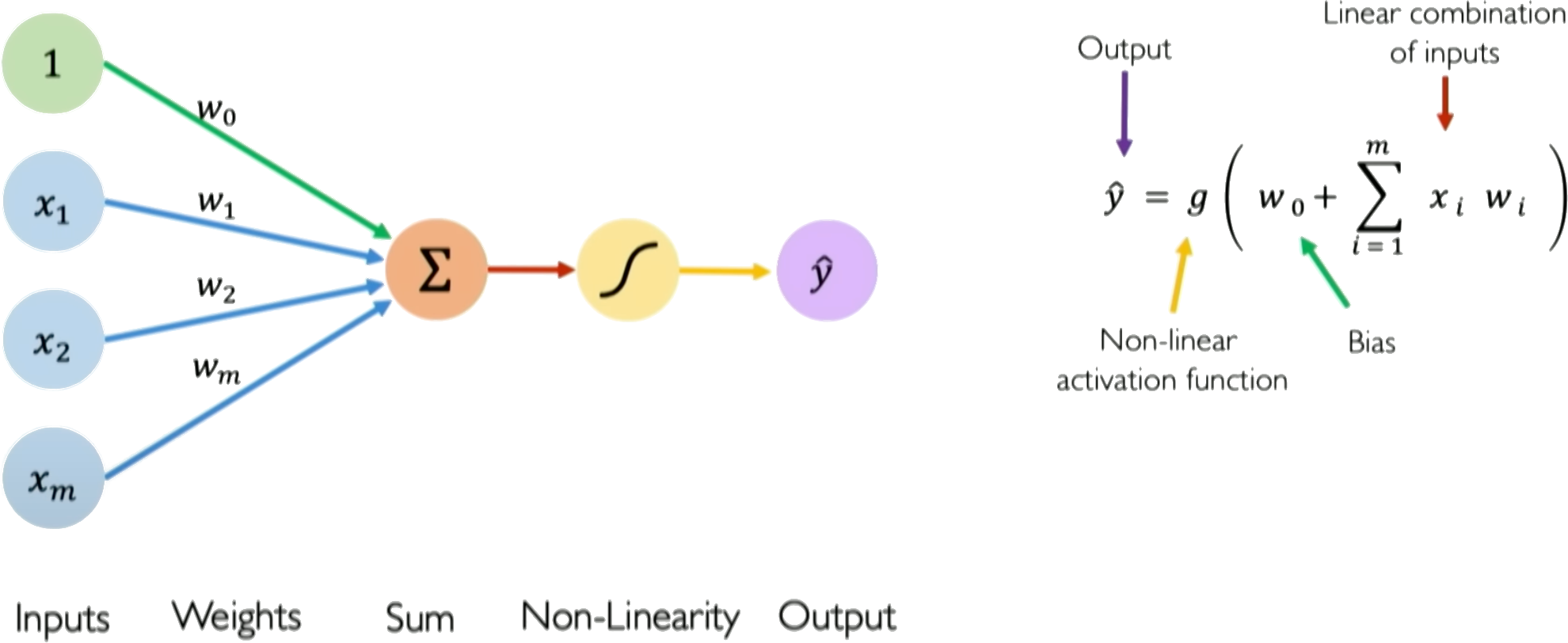
The key insight is that only the weights and biases are trainable. The activation function $`g`$ is fixed—chosen before training and never modified. This means the network learns by adjusting linear combinations; all nonlinearity comes from the fixed activation function applied to these linear combinations. Training minimizes a loss function measuring prediction error. For regression, the mean squared error is typical:
\begin{equation}
\mathcal{L} = \frac{1}{N}\sum_{i=1}^{N}(y_i - \hat{y}_i)^2
\end{equation}Weights update iteratively via gradient descent, $`w \leftarrow w - \eta \nabla_w \mathcal{L}`$, where $`\eta`$ is the learning rate. Backpropagation computes these gradients efficiently by applying the chain rule layer by layer, working backward from output to input. Stacking neurons into multiple layers allows the network to learn hierarchical features, with early layers capturing simple patterns and deeper layers combining these into complex relationships.
Activation Functions and Feature Normalization
The choice of activation function determines how the network represents nonlinearity. Common options include ReLU ($`g(z) = \max(0,z)`$), tanh ($`g(z) = \tanh(z)`$, outputs between $`-1`$ and $`+1`$), and sigmoid ($`g(z) = 1/(1+e^{-z})`$, outputs between 0 and 1). Each has a sensitive region where small changes in input produce meaningful changes in output—and a saturated region where the function flattens and gradients vanish.
For tanh and sigmoid, the sensitive region lies roughly where $`|z| < 2`$. Outside this range, outputs saturate near their limits and gradients approach zero. For ReLU, the function is zero for all negative inputs (gradient also zero) and linear for positive inputs. When inputs fall outside these sensitive regions, neurons stop learning—gradients vanish, and weight updates become negligible. This is the “dead neuron” problem.
Feature normalization keeps inputs in the sensitive region. When features differ by orders of magnitude—depth in meters versus effective stress in kilopascals—the weighted sum $`w_1 z + w_2 \sigma'`$ can easily produce values of hundreds or thousands, pushing neurons deep into saturation. Z-score normalization solves this problem.
\begin{equation}
x_{\text{norm}} = \frac{x - \mu_{\text{train}}}{\sigma_{\text{train}}}
\end{equation}This centers features at zero with unit variance, ensuring that typical inputs produce weighted sums in the sensitive region of activation functions. Critically, normalization statistics must come from training data only—using test data leaks information and inflates reported accuracy.
The Extrapolation Problem
Consider a mat foundation design for a high-rise building with settlement measurements from a previous structure on the same site loaded up to 200 kPa. The new building will impose 350 kPa. Can a neural network trained on the existing settlement data confidently predict settlement under the higher loading? The answer is no, and understanding why reveals the first fundamental limitation of machine learning for geotechnical problems.
Let’s build intuition through Terzaghi consolidation settlement—a curve every geotechnical engineer has plotted. Settlement follows $`S(t) = S_\infty(1 - e^{-\alpha t})`$, where $`S_\infty`$ is the final settlement and $`\alpha`$ controls the rate. The curve starts at zero, rises steeply at first, then gradually approaches its asymptote.
We ran a direct experiment. Take 20 settlement observations from the first two years ($`t = 0`$ to $`t = 2`$ years) representing typical measurements from settlement plates after loading. Train three multi-layer perceptrons (MLPs), each with two hidden layers and 32 neurons per layer, using three different activation functions: ReLU ($`\max(0,z)`$), tanh (squashes between -1 and 1), and sigmoid (squashes between 0 and 1). All three networks learn to fit this training data beautifully, achieving mean squared error below 6 mm$`^2`$—they track the measurements almost perfectly (2).
Now ask the networks to predict settlement from year 2 to year 10—extrapolation beyond the training domain. With $`S_\infty = 100`$ mm and $`\alpha = 0.5`$ year$`^{-1}`$, the true settlement at year 10 is 99.3 mm. What do the networks predict?
The ReLU network predicts 264 mm at year 10—an error of 165 mm, extrapolating linearly upward without bound (RMSE = 87.6 mm over the full 10-year span). This happens because ReLU is piecewise linear; outside the region where the network learned nonlinear combinations, it can only produce linear growth. The tanh and sigmoid networks fail differently: they predict 60-61 mm at year 10, underestimating by 39% (RMSE = 31 mm) because both activation functions saturate, making the networks predict that settlement has nearly stopped even though consolidation is still progressing.
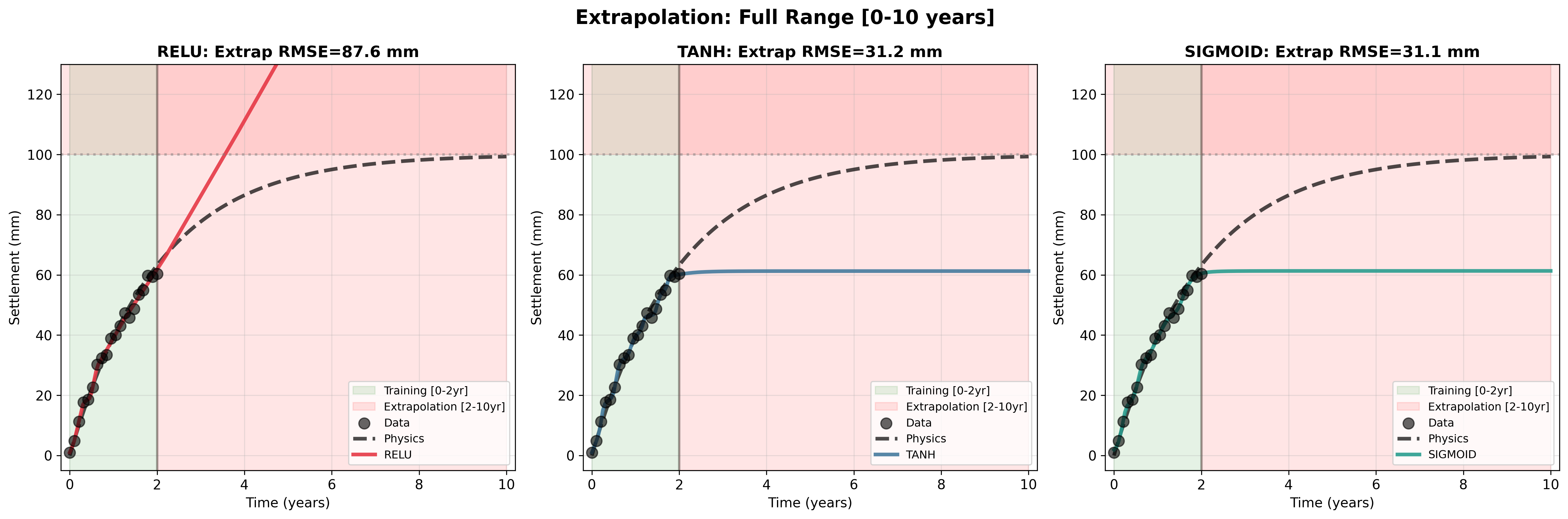
All three networks achieved low training error, yet all three failed catastrophically when asked to extrapolate. This is not a hyperparameter tuning problem or a “we need more data” problem. This is a fundamental limitation of how neural networks represent functions.
Why does this happen? Neural networks are interpolation machines, not extrapolation machines. The mathematical guarantee—the universal approximation theorem —states that a sufficiently wide network can approximate any continuous function on a compact domain. That is, within the training envelope. It says nothing about reliability beyond that domain. The network learned to fit the shape of an exponential curve between $`t = 0`$ and $`t = 2`$ years. Outside that range, the network’s prediction is mathematically unconstrained. Without physical constraints, the network has no reason to prefer the asymptotic exponential decay of Terzaghi’s equation over unbounded linear growth (ReLU) or premature saturation (tanh, sigmoid).
Training accuracy does not imply extrapolation reliability. Training loss curves cannot reveal whether a neural network will perform well on extrapolation. This applies to all multi-layer perceptrons, regardless of activation function, architecture depth or width, or training algorithm. The problem is structural, not parametric.
This problem compounds in higher dimensions. Balestriero et al. prove a remarkable result: in high-dimensional spaces, almost every new query point falls outside the convex hull of training data. Interpolation almost surely never happens. Consider our liquefaction classifier with just four features: peak ground acceleration $`a_{\max}`$, shear wave velocity $`V_{s30}`$, groundwater depth $`d_w`$, and distance to waterway $`d_r`$. With 1000 training cases, 41% of new points lie near the boundary of the training data. Add more features—soil layer depths, fines content, earthquake magnitude, distance to fault—and the fraction approaches 100%. Nearly all predictions become extrapolations, where the network has no guarantees of reliability.
This is not a geotechnical-specific problem, but geotechnical engineering makes it worse. We must predict beyond observed conditions: settlement under loads exceeding previous experience, slope stability during a 100-year storm that has not yet occurred, liquefaction during an earthquake larger than the design basis events in the training data, foundation performance on a new soil profile not represented in calibration data. We cannot “add more training data” to cover extreme events that have not happened. This is not a data scarcity problem solvable by collecting more samples—it is a fundamental limitation of the approach.
Spatial Autocorrelation: The Generalization Fallacy
Consider 200 CPT soundings from five sites around a city, used to train a classifier that identifies liquefaction-susceptible layers from tip resistance $`q_c`$, sleeve friction $`f_s`$, and pore pressure $`u_2`$. Following standard machine learning practice, the soundings are randomly shuffled, 160 used for training (80%), and 40 held out for testing (20%). The classifier achieves 92% test accuracy.
That 92% is misleading. The problem is that random splitting ignores spatial structure in the data, violating the independence assumption that underlies the train-test methodology.
Soil properties are spatially correlated—a well-established principle in geotechnical practice. A CPT sounding at one location reveals soil conditions nearby, not conditions kilometers away. Geostatistical models quantify this through semivariograms with correlation lengths of 50-100 meters horizontally . Clay content measured at one location will be similar to a measurement 10 meters away; at 100 meters, values become independent.
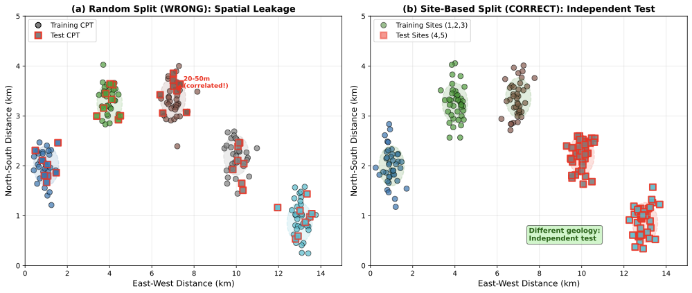
Random data splitting ignores this correlation. Randomly splitting 200 CPT soundings from five sites (40 soundings per site) results in each site contributing roughly 32 training soundings and 8 test soundings. The catch: those 8 test soundings from Site 1 lie 20-50 meters from the 32 training soundings at the same site. They are not independent. The test soundings fall within the spatial correlation ellipse of training soundings (3a). The classifier has not learned to generalize to new sites with different geology—it has learned the specific geological signature of the five training sites, and the test data simply confirms it can interpolate within those same sites.
 />
/>
The correct approach is site-based splitting (3b). For e.g., use Sites 1, 2, and 3 (120 soundings) for training and Sites 4 and 5 (80 soundings) for testing. Now the test sites are geologically independent—they have different stratigraphy, different depositional history, different groundwater conditions. Alternatively, use k-fold site cross-validation: train on four sites, test on the fifth, repeat for all combinations. This provides an honest estimate of generalization to a genuinely new site, which is what matters when deploying a classifier at Site 6 next year.
The difference in reported accuracy is dramatic. For CPT soil classification , random splitting gives 90-95% test accuracy. Site-based splitting gives 70-80% accuracy—a difference that matters when designing a foundation based on the predicted soil profile. The 20-point drop is not noise; it is the difference between interpolating within known sites and genuinely generalizing to new geology.
Traditional geotechnical methods handle spatial correlation naturally because they were developed by people who dug in the ground. We use kriging to interpolate soil properties between boreholes, explicitly accounting for correlation structure. We use random field models in finite element analysis, specifying correlation lengths and anisotropy based on geological knowledge. We never assume that a measurement at one location is independent of measurements 20 meters away—that would be geological nonsense. Machine learning offers no built-in mechanism to respect spatial correlation. This must be imposed manually through careful cross-validation design, or the model will fail when it encounters a new site with geology not represented in the training data.
A related validation issue is class imbalance. High-consequence events are rare: a typical liquefaction database might contain 200 liquefaction cases (4%) and 4,800 non-liquefaction cases (96%). A classifier predicting “no liquefaction” for every site achieves 96% accuracy while missing every actual failure. The solution is to evaluate models using recall (fraction of actual failures detected) and F1-score rather than accuracy, and to recognize that in geotechnical applications, missing a failure (false negative) is far more costly than a false alarm (false positive).
Physics-Informed Neural Networks: The Computational Cost
What if we teach the neural network to obey the physics? Instead of training purely on data, we add the governing equations as a constraint in the loss function. The network must simultaneously fit measurements and satisfy the wave equation, the consolidation equation, or whatever differential equation governs the problem. This should fix the extrapolation problem, because now the network cannot produce physically impossible behavior. The idea is called physics-informed neural networks (PINNs), and it has generated hundreds of papers since Raissi et al. introduced it in 2019 . Recent geotechnical applications include pile-soil interaction , seismic site response , and general geoengineering problems .
Let’s see how it works for wave propagation, the fundamental equation for seismic site response analysis in geotechnical earthquake engineering. The 1D wave equation is:
\begin{equation}
u_{tt} = c^2 u_{xx}
\end{equation}where $`u(x,t)`$ is displacement, $`x`$ is position, $`t`$ is time, and $`c`$ is wave velocity (shear wave velocity $`V_s`$ for SH-waves in soil). To solve this with a PINN, we train a neural network $`f_\theta(x,t)`$ that takes coordinates $`(x,t)`$ as input and outputs a single scalar—the displacement $`u`$ at that point. The network knows nothing about derivatives; it simply maps coordinates to displacement values.
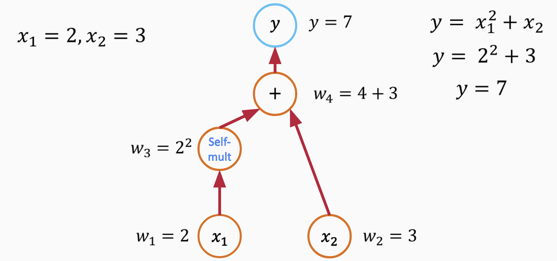
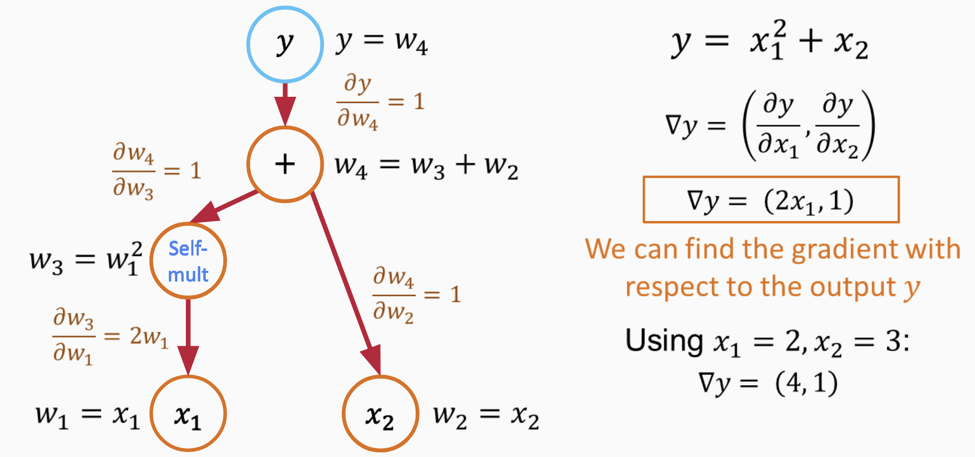
To enforce the PDE, we need the second derivatives $`u_{tt}`$ and $`u_{xx}`$. Since the network is a composition of differentiable operations (matrix multiplications and activation functions), we can compute these derivatives exactly using automatic differentiation (AD). AD applies the chain rule through the network’s computational graph, giving us $`\partial u/\partial t`$, $`\partial^2 u/\partial t^2`$, $`\partial u/\partial x`$, and $`\partial^2 u/\partial x^2`$ at any point. We discuss AD in detail later, but the key point is that these derivatives are exact (to machine precision), not finite-difference approximations.
With derivatives in hand, we minimize a composite loss function:
\begin{equation}
\mathcal{L} = \mathcal{L}_{\text{PDE}} + \lambda_{\text{IC}} \mathcal{L}_{\text{IC}} + \lambda_{\text{BC}} \mathcal{L}_{\text{BC}}
\end{equation}The first term $`\mathcal{L}_{\text{PDE}} = \left| u_{tt} - c^2 u_{xx} \right|^2`$ penalizes violations of the wave equation, evaluated at collocation points sampled throughout the domain. The other terms $`\mathcal{L}_{\text{IC}}`$ and $`\mathcal{L}_{\text{BC}}`$ enforce initial conditions (displacement at $`t=0`$) and boundary conditions (displacement at domain edges). The weights $`\lambda_{\text{IC}}`$ and $`\lambda_{\text{BC}}`$ control how strongly we enforce each constraint. 4 shows the PINN architecture for 1D wave propagation.
The promise is compelling. Train the network once on sparse sensor data, and it will produce solutions that both fit the data and obey wave physics everywhere. This could apply to seismic site response, where accelerometer measurements exist at a few depths but ground motion predictions are needed at all depths. Should we abandon our finite difference codes?
A fundamental limitation becomes apparent when we consider what “training” means here. The PINN learns weights $`\theta`$ that make $`f_\theta(x,t)`$ satisfy this specific PDE with these specific initial and boundary conditions. Change the initial pulse shape, move a boundary, or alter the velocity profile, and the trained network is useless—it must be retrained from scratch. Each forward problem requires a fresh optimization. Compare this to a finite difference solver, which handles any initial condition, any boundary condition, and any velocity profile by simply changing input arrays. The FD solver is a general-purpose tool; a trained PINN is a single-use solution.
The critical word in that description is approximately. The PDE enters as a soft constraint—penalized but not strictly enforced. The network tries to minimize the PDE residual, but there is no guarantee it will succeed. Three problems arise. First, the PDE term and boundary terms have vastly different magnitudes, causing ill-conditioning. Second, networks preferentially learn smooth functions and miss sharp gradients, a phenomenon called spectral bias. Third, the optimizer must juggle competing objectives, leading to multi-objective imbalance .
There is also a subtler issue connecting back to our earlier discussion of extrapolation. PINNs evaluate the PDE residual at collocation points—a finite set of $`(x,t)`$ coordinates sampled throughout the domain. The network learns to satisfy the PDE at these points and interpolates between them. This may appear to solve the extrapolation problem since physics rather than data constrains the solution. But the network is still an MLP with the same activation functions and the same mathematical structure. Outside the collocation domain—at times beyond the training window or spatial locations not covered—the network extrapolates with the same failure modes we observed for settlement prediction. The physics constraint applies only where we evaluate it. Beyond those points, the network reverts to unconstrained extrapolation.
The Test: 1D Wave Equation
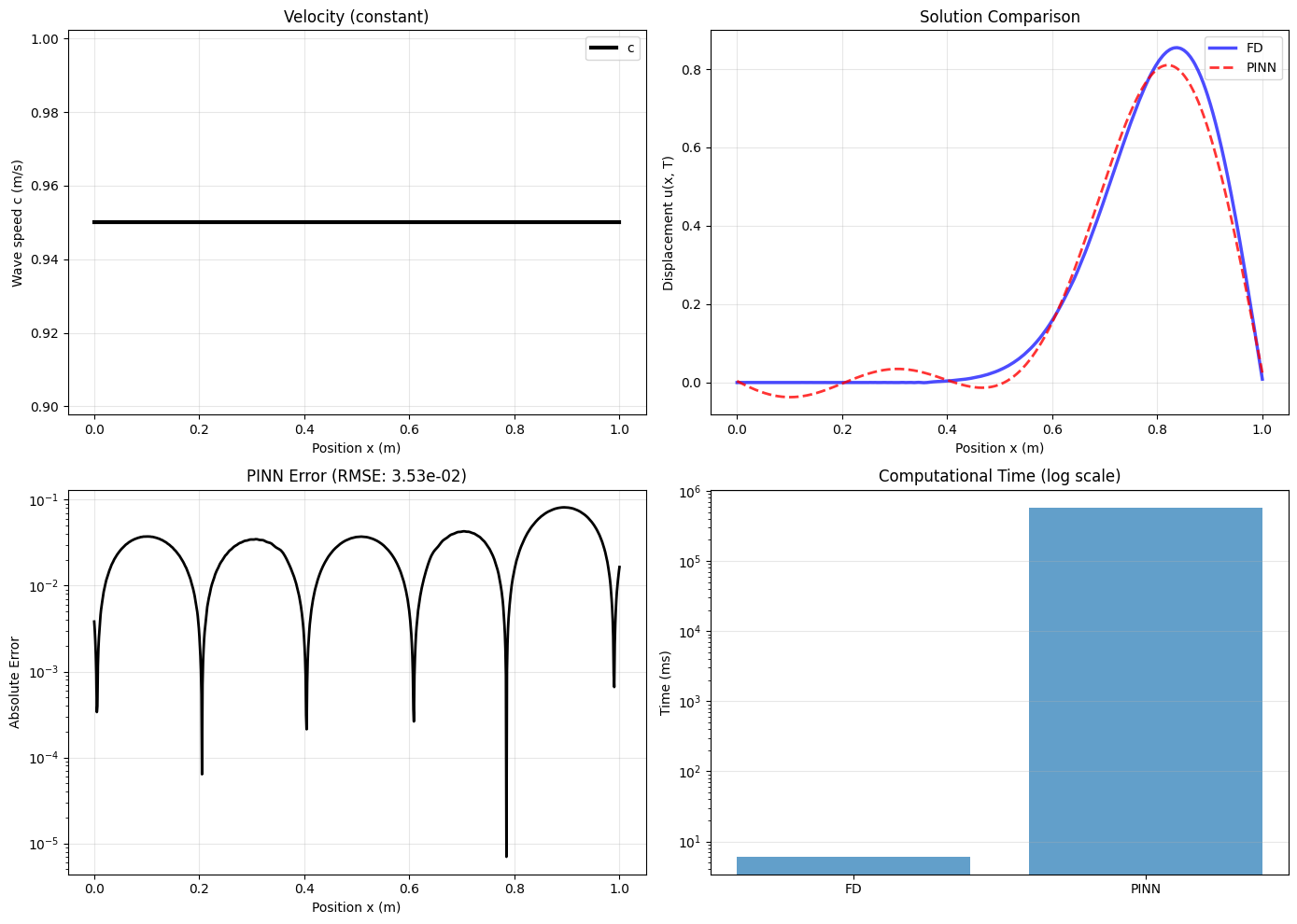
Let’s test PINNs on the simplest possible wave propagation problem: a 1D domain from $`x = 0`$ to $`x = 1`$ meter with constant wave velocity $`c = 0.95`$ m/s (typical shear wave velocity in soft clay). We start with a Gaussian pulse at the center: $`u(x,0) = \exp(-25(x-0.5)^2)`$, and apply zero displacement at both boundaries. This represents a pulse propagating through a soil column—simplified, but captures the essential physics.
We compare two approaches. First, a standard finite difference (FD) solver with 1000 spatial grid points and 5000 time steps using explicit central differences—this is what every geotechnical seismic code uses. Second, a PINN with 4 hidden layers, 128 neurons per layer, and sine activation functions (recommended for wave problems). We train the PINN for 9000 iterations using the Adam optimizer followed by L-BFGS refinement.
The finite difference solver completes in 6.4 milliseconds. The PINN training takes 581 seconds—nearly ten minutes. The PINN is 90,781 times slower.
Is the PINN at least more accurate? No. Comparing solutions at final time $`t = 2.5`$ seconds, the root-mean-square difference between PINN and FD is $`3.5 \times 10^{-2}`$. The finite difference solution satisfies the wave equation to machine precision (error $`< 10^{-15}`$). The PINN satisfies the PDE with residual around $`10^{-3}`$—better than a pure data-driven network, but nowhere near the accuracy of FD. 5 shows the actual waveform comparison and error distribution.
1 summarizes the performance quantitatively.
| Problem Type | Method | Time (s) | RMSE | Speedup |
|---|---|---|---|---|
| Forward | Finite Difference | 0.0064 | < 10−15 | 1× |
| PINN | 581 | 0.035 | 90,781× slower | |
| Inverse | Auto-Differentiation | 32 | 0.0056 | 1× |
| PINN | ∼30–60 | 0.01–0.05 | Similar |
Architecture details. Our PINN uses a fully-connected neural network with 4 hidden layers of 128 neurons each. The input layer takes spatiotemporal coordinates $`(x, t)`$ normalized to $`[-1, 1]`$. We employ sine activation functions (SIREN architecture) with frequency parameter $`\omega_0 = 30`$ to capture high-frequency wave oscillations—standard ReLU or tanh activations fail to represent oscillatory solutions. The output is the scalar field $`u(x,t)`$. Training uses the Adam optimizer with learning rate $`10^{-3}`$ for 9000 iterations, requiring careful tuning of learning rate schedules and loss weighting coefficients.
Why does training take so long, and why is accuracy so poor? The loss function tries to satisfy three competing objectives simultaneously: minimize PDE violations, match initial conditions, and enforce boundary conditions. These terms have vastly different magnitudes. In our experiment, the PDE residual drops quickly to $`10^{-2}`$, but the boundary condition term stagnates at $`10^{-3}`$ and initial conditions hover around $`10^{-4}`$. The optimizer cannot balance these competing demands effectively. Wang et al. call this the “multi-objective imbalance problem”—solutions satisfy the PDE roughly but violate boundaries, or vice versa.
Researchers have proposed fixes such as adaptive loss weighting, curriculum learning (train on easier sub-problems first), and separate networks for different physics components. These help marginally but add complexity. Meanwhile, the finite difference solver—mature technology with 60 years of development—just works. Our FD code is 80 lines; the PINN code is 500+ lines plus extensive hyperparameter tuning.
Automatic Differentiation and Differentiable Programming
Before exploring inverse problems with PINNs, we must understand automatic differentiation (AD)—a superior alternative that transforms traditional solvers into differentiable programs. Automatic differentiation is a family of techniques for computing derivatives of functions specified by computer programs. Unlike numerical differentiation (finite differences) which approximates derivatives through perturbations, or symbolic differentiation which operates on mathematical expressions, AD exploits the fact that every computer program executes a sequence of elementary arithmetic operations and elementary functions. By applying the chain rule repeatedly to these operations, AD computes exact derivatives (up to machine precision).
AD operates in two modes, forward and reverse (6). Forward mode computes derivatives in the same direction as the program execution, efficiently computing gradients when outputs outnumber inputs. Reverse mode, also called backpropagation in neural network contexts, computes derivatives by traversing the computation graph backward, efficiently handling cases where inputs vastly outnumber outputs—exactly the scenario in typical inverse problems where we have many parameters but few objective function outputs.
This capability transforms numerical solvers into differentiable programs—computational tools that not only produce outputs but also provide exact gradients of those outputs with respect to inputs . For geotechnical engineering, this means we can wrap finite difference codes for consolidation, wave propagation, or seepage in automatic differentiation frameworks (JAX, PyTorch) and immediately gain gradient-based optimization capabilities for parameter estimation and inverse problems. The solver becomes an oracle that, when queried with parameters, returns both the solution and exact sensitivities with respect to all inputs. This paradigm—differentiable programming—extends beyond machine learning to enable gradient-based optimization of traditional computational physics methods.
Inverse Problems: Automatic Differentiation vs. PINNs
Now we can fairly compare automatic differentiation through traditional solvers against physics-informed neural networks for inverse problems.
Consider the same wave equation problem, but now the velocity profile $`c(x)`$ is unknown. We parametrize it as a linear function $`c(x) = c_0 + \alpha x`$, giving just two unknowns. True values are $`c_0 = 0.9`$ m/s, $`\alpha = 0.3`$ m$`^{-1}`$. We place 20 sensors along the domain and record the final wavefield $`u(x, t_f)`$ with 1% Gaussian noise added to simulate measurement error.
Automatic Differentiation Approach: We wrap the finite difference solver in JAX and compute $`\nabla_{c_0, \alpha} \mathcal{L}`$ where $`\mathcal{L} = \|u_{\text{sim}}(x; c_0, \alpha) - u_{\text{obs}}(x)\|^2`$. Starting from initial guess $`c_0 = 0.85`$ m/s, $`\alpha = 0.2`$ m$`^{-1}`$, we run Adam optimizer for 2000 iterations. Total time is 32 seconds. We recover $`c_0 = 0.9106`$ m/s and $`\alpha = 0.2795`$ m$`^{-1}`$ (true values: $`c_0 = 0.9000`$ m/s, $`\alpha = 0.3000`$ m$`^{-1}`$), yielding relative errors of 0.56% and 6.8% respectively. Each iteration runs the forward solver once and backpropagates exact gradients through the entire computation—no approximation, no soft constraints, no neural network training, no multi-objective balancing. The solver enforces physics exactly at every step (to discretization error only).
PINN Inverse Approach: The inverse PINN simultaneously tries to (1) match sensor measurements, (2) satisfy the PDE, and (3) recover the velocity parameters. This creates a difficult multi-objective optimization problem with competing loss terms.
7 compares both approaches directly. While the inverse PINN achieves reasonable velocity recovery (RMSE $`3.18 \times 10^{-2}`$), automatic differentiation converges faster and more reliably. The AD approach requires approximately 80 lines of JAX code; the PINN implementation requires 500+ lines plus extensive hyperparameter tuning.
There are scenarios where PINNs could be useful, though they are narrow. With scattered sensor measurements at irregular locations (not on a grid), fitting a mesh is awkward and PINNs provide a mesh-free alternative. For assimilating sparse, noisy field data while enforcing known physics constraints, PINNs offer a framework for data assimilation. For inverse problems, however, automatic differentiation through the forward solver should be tried first.
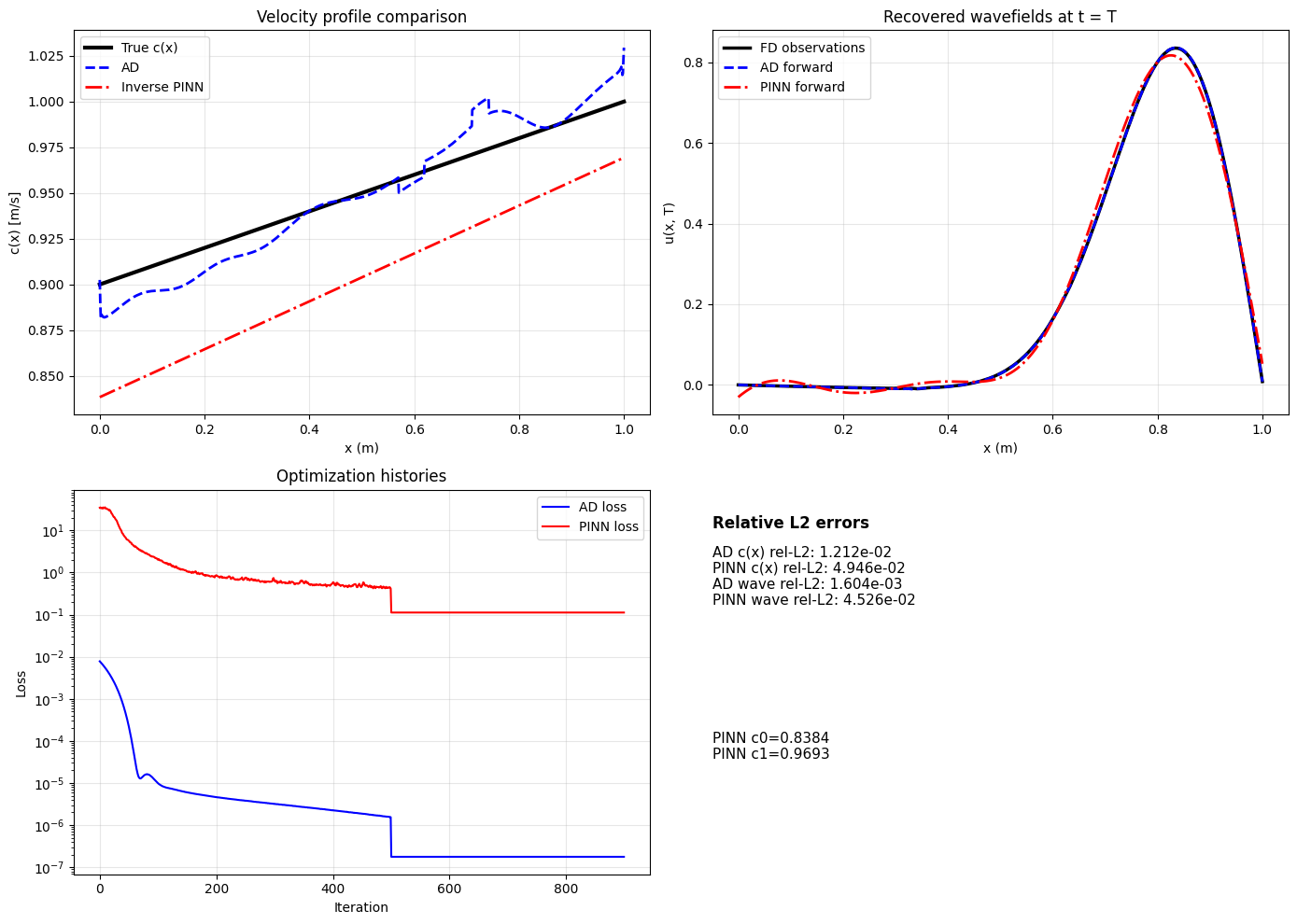
notebooks/ad-pinn-fwi.ipynb). Top
left: velocity profile comparison showing true profile (constant c = 0.95 m/s) versus recovered
profiles from automatic differentiation (AD) and inverse PINN. Top
right: recovered waveforms at c = 1 plateau. Bottom panels show
optimization histories for both methods. While the inverse PINN achieves
reasonable velocity recovery (RMSE 3.18 × 10⁻²), automatic
differentiation through the forward solver converges faster and more
reliably. For inverse problems, try AD first before resorting to
PINNs.For forward problems on regular domains with known parameters, finite difference or finite element wins decisively. Do not use PINNs when the solver runs in seconds. The 90,000× slowdown makes no engineering sense.
Operator Learning: The Data Requirement for DeepONet
A different approach trains a network to learn the entire mapping from inputs to outputs, not just for one specific case, but for all possible cases. Consider mat foundation design. Given load pattern $`p(x)`$ along the foundation, what deflection $`w(x)`$ results? Normally the governing differential equation must be solved for each new load pattern. But what if a network could be trained once on many load-deflection pairs, then queried instantly for any new load pattern?
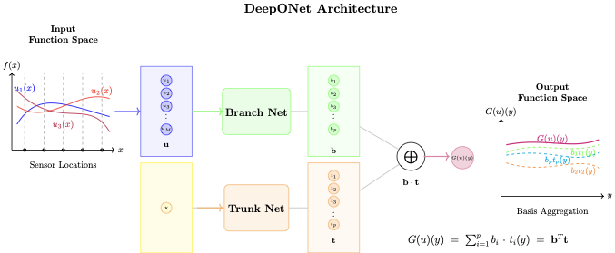
This is called operator learning. Deep Operator Networks (DeepONet) and Fourier Neural Operators (FNO) are the leading architectures. DeepONet uses two networks: a branch network encodes the input function $`p(x)`$ sampled at fixed sensor locations, and a trunk network encodes the query locations where output is desired. Multiply their outputs and sum to get predictions $`w(x)`$ everywhere. Train on thousands of input-output function pairs.
The promise is computational amortization—invest time training offline once, then enjoy instant online predictions forever. For a parametric study evaluating hundreds of load configurations, this could save enormous time. Should we use this for mat foundation design?
Numerical Experiment: Beam on Elastic Foundation
The governing equation for a beam on elastic foundation (Winkler model) is:
\begin{equation}
EI w^{(4)} + k w = p(x)
\end{equation}where $`w(x)`$ is deflection, $`p(x)`$ is distributed load, $`EI = 5 \times 10^6`$ N·m$`^2`$ is flexural rigidity, and $`k = 10^5`$ N/m$`^2`$ is foundation modulus (modulus of subgrade reaction). Boundary conditions are simply supported: $`w(0) = w(L) = w''(0) = w''(L) = 0`$ with $`L = 10`$ m.
We generate 5000 random load profiles (combinations of Gaussian bumps, Fourier modes, and polynomials) and solve the fourth-order differential equation using finite difference with 128 grid points and five-point stencil for the fourth derivative. This creates the training set.
Architecture details. The DeepONet consists of two parallel networks: a branch network that encodes the input function $`p(x)`$ and a trunk network that encodes query locations. The branch network takes the load sampled at 128 fixed sensor locations as input, processes it through 3 hidden layers of 256 neurons each with tanh activation, and outputs a 256-dimensional latent representation. The trunk network takes a single spatial coordinate $`x`$ as input, processes it through 3 hidden layers of 256 neurons (also tanh), and outputs a corresponding 256-dimensional representation. The final prediction is the dot product of these two representations: $`\hat{w}(x) = \sum_{k=1}^{256} b_k \cdot t_k`$, where $`b_k`$ are branch outputs and $`t_k`$ are trunk outputs. This factorization allows the network to learn a basis of deflection modes (8). We train for 8000 iterations using AdamW optimizer with cosine learning rate decay starting from $`10^{-3}`$.
 style="width:85.0%" />
The FD solver completes each solution in 0.11 ms. DeepONet training requires 203 seconds, and inference takes 5.45 ms per query with normalized test MSE of $`5.9 \times 10^{-3}`$. The DeepONet is 50 times slower at inference than the direct solver. For 10,000 load cases (a generous parametric study), FD total time is 1.1 seconds while DeepONet requires 258 seconds—235 times slower overall. To break even on total time would require roughly 1.8 million evaluations. No geotechnical project evaluates a single beam configuration 1.8 million times.
When Does Operator Learning Make Sense?
How expensive must the forward solver be to justify operator learning? 2 provides guidance.
| Forward Solver | Time/ | Training | Queries to | Typical Use Case |
| Solve | Overhead | Break Even | ||
| FD (Winkler beam) | 0.1 ms | 203 s | 1,800,000 | Use FD |
| 2D FEM (settlement) | 1 s | 203 s | 200 | Use FEM |
| 3D FEM (parametric) | 60 s | 203 s | 3-4 | Consider DeepONet |
| Coupled 3D (complex) | 3600 s | 203 s | $`<`$1 | DeepONet justified |
DeepONet Break-Even Analysis for Geotechnical Applications
For typical geotechnical problems with fast solvers—1D consolidation (microseconds), 2D seepage (seconds), elastic settlement (seconds)—operator learning is overkill. The training cost and potential for error outweigh any inference speedup. Only when the forward solver takes minutes to hours and hundreds of evaluations are needed does operator learning become competitive.
Operator networks make sense when the forward solver is genuinely expensive (minutes to hours per solve), rapid queries are needed for real-time applications such as digital twins or monitoring systems, and the input-output relationship is complex enough that reduced-order models struggle. Examples might include 3D finite element models of complex soil-structure interaction where each solve takes 30 minutes and 10,000 parameter combinations need exploration. Even then, reduced-order models and surrogate methods developed over decades in structural mechanics (proper orthogonal decomposition, kriging, polynomial chaos expansion) should be considered as simpler alternatives.
Limitations of DeepONet
Beyond computational break-even, DeepONet has structural limitations that restrict its applicability. Training requires thousands of input-output function pairs. Our beam experiment used 5,000 load-deflection pairs, each requiring a forward solve. For problems where generating training data is expensive—the same problems where DeepONet might help—this creates a chicken-and-egg problem where training data generation dominates the total cost.
The branch network samples the input function at fixed sensor locations. Once trained, the network expects input functions sampled at exactly those locations. If sensor placement changes, a common occurrence in field monitoring, the network must be retrained. Similarly, DeepONet learns the operator for a specific domain geometry. Change the beam length, add a notch, or modify boundary locations, and the trained network is invalid. Unlike finite element solvers that handle arbitrary geometries through mesh generation, DeepONet embeds the geometry into its learned weights.
DeepONet also breaks translational invariance. PDEs like the wave equation and beam equation have this symmetry—shifting the entire domain in space does not change the solution. A beam from $`x = 0`$ to $`x = L`$ behaves identically to one from $`x = 2`$ to $`x = 2 + L`$ under the same loading. DeepONet does not respect this; it treats these as entirely different problems requiring separate learned mappings. This increases the effective complexity of the learning problem and the data required to cover the input space.
These limitations suggest the ideal application for operator learning: digital twins where geometry and material properties are fixed but boundary and initial conditions vary. Consider a specific bridge or building instrumented with sensors. The structure does not change, so geometry is fixed. Material properties are characterized once. But loading conditions vary continuously—traffic, wind, seismic events. Training DeepONet or a PINN on this fixed geometry with varied loadings creates a fast surrogate for real-time structural health monitoring. Zhang et al. demonstrated this approach for real-time settlement prediction during tunnel construction, fusing simulation and monitoring data through a multi-fidelity DeepONet. The upfront training cost amortizes over years of continuous queries, and the fixed sensor locations match the network’s architectural constraints.
Graph Network Simulators: Learning Particle Dynamics
Graph Network Simulators (GNS) take a different approach to operator learning . Related methods include MeshGraphNets for mesh-based simulations . Rather than learning a fixed mapping between function spaces like DeepONet, GNS learns the local interaction laws governing particle dynamics. The method discretizes the physical domain with nodes representing material points and edges connecting neighboring particles. By learning how particles influence their neighbors, GNS can simulate complex phenomena including granular flows, fluid dynamics, and deformable solids.
The architecture follows an encode-process-decode structure. The encoder embeds particle states (position, velocity, material properties) and boundary information into latent node and edge features. The processor applies multiple rounds of message passing, where each node aggregates information from its neighbors through learned functions—this is where the network learns the physics of local interactions. The decoder extracts accelerations from the processed node features. A simple Euler integration step then updates positions and velocities for the next timestep. The network trains on trajectories from high-fidelity simulations (DEM, MPM) by minimizing the error between predicted and actual accelerations.
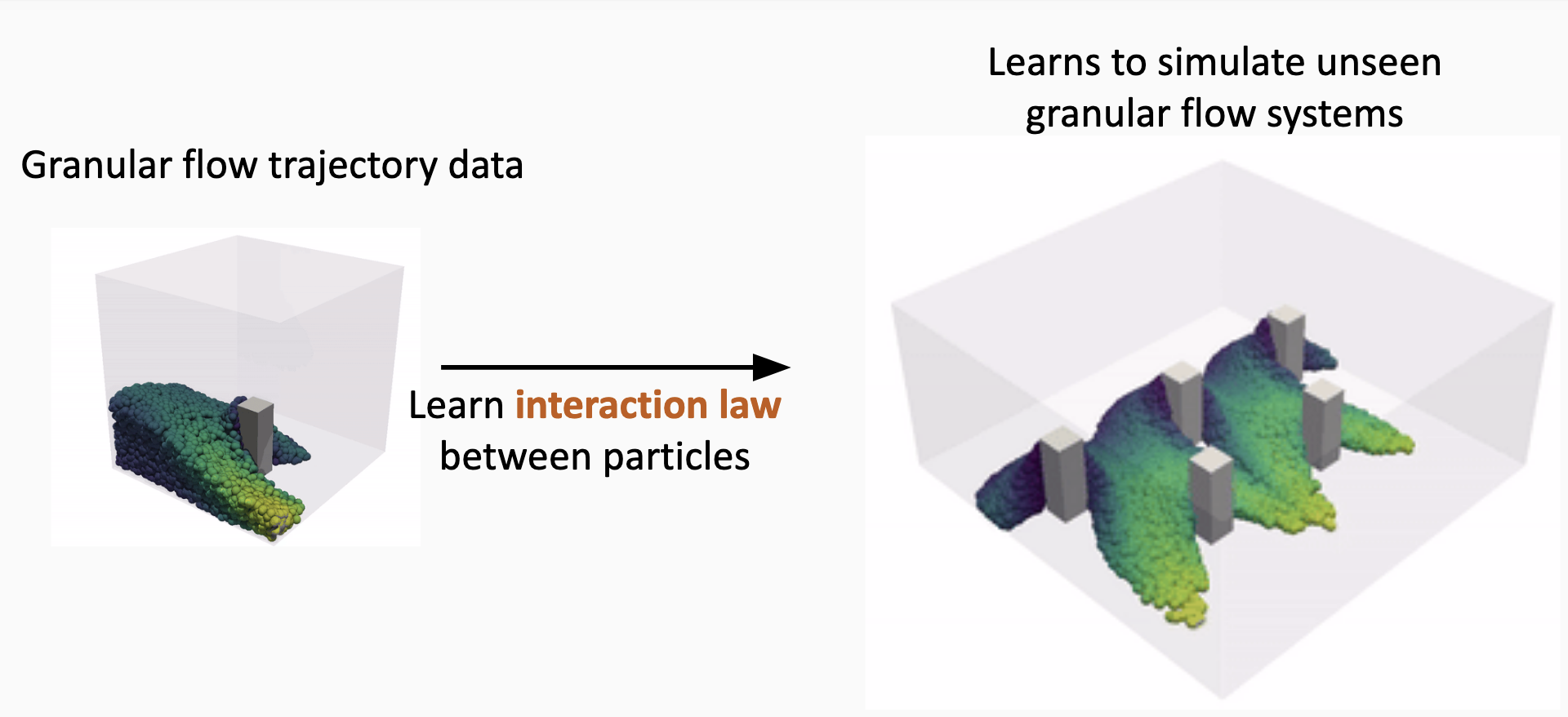
Unlike DeepONet, GNS is geometry-agnostic. The graph structure adapts to any particle configuration, and because the learned interaction laws are local, a model trained on one geometry can generalize to different boundary conditions and domain shapes. 9 illustrates this capability: a GNS trained on granular column collapse with a single barrier configuration accurately predicts flow dynamics with multiple barriers, different barrier positions, and barrier shapes not seen during training . This generalization arises because the network learns the fundamental particle-particle and particle-boundary interactions rather than memorizing specific configurations.
Choi and Kumar applied GNS to granular flows relevant to geotechnical engineering, demonstrating speedups of several thousand times over Material Point Method (MPM) simulations while maintaining accuracy within 5% for column collapse problems. They further developed differentiable GNS for inverse analysis, using automatic differentiation through the learned simulator to estimate material parameters from observed flow behavior .
Despite these promising results, several limitations constrain GNS applicability. First, GNS requires warmstarting—it cannot begin from an arbitrary initial configuration but needs a few timesteps of velocity history to initialize predictions. This precludes instantaneous queries and complicates integration with other simulation components.
Second, granular materials exhibit path-dependent behavior that GNS cannot capture. Current stresses depend on the entire loading history, not just the current configuration. GNS receives only the last few timesteps (typically 3-5 frames) as input. A sample loaded in compression then shear behaves differently than one loaded in shear alone, even if current configurations are identical. GNS trained on monotonic loading cannot generalize to cyclic loading or stress reversals .
Third, memory limits scaling to realistic problem sizes. For $`N`$ particles with average degree $`k`$ neighbors, GNS requires $`O(Nk)`$ memory per timestep. Training requires storing activations for backpropagation through time. For a 1000-timestep simulation with $`10^6`$ particles, memory requirements exceed 100 GB. Reported demonstrations use $`10^3`$ to $`10^4`$ particles—two to three orders of magnitude smaller than the $`10^6`$ to $`10^7`$ particles needed for foundation bearing capacity or shear band localization studies.
Fourth, distributed training is difficult. Scaling GNS across multiple GPUs requires domain decomposition of every training trajectory, with ghost nodes at partition boundaries to maintain message passing. The dynamic nature of granular flow means particles migrate between partitions, requiring either conservative static partitioning (inefficient) or dynamic repartitioning (complex). Unlike image data that parallelizes trivially across samples, graph-structured particle data couples spatially in ways that resist simple distribution.
For typical geotechnical DEM problems with $`10^4`$ particles running in minutes, the training cost, data requirements, and accuracy limitations of GNS do not justify the investment. The method shows more promise for problems where traditional solvers take hours and geometric generalization is valuable.
Discussion and Conclusion
Our experiments reveal a clear hierarchy. Multi-layer perceptrons fail catastrophically on extrapolation—the common case in geotechnical engineering. Physics-informed neural networks are 90,000 times slower than finite difference with larger errors, offering no advantage when solvers run in seconds. Deep operator networks require thousands of training simulations for inference that remains slower than direct solution, breaking even only after millions of evaluations. Only automatic differentiation through traditional solvers succeeds for inverse problems, providing exact gradients and sub-percent parameter recovery. These are not marginal differences. When a method is $`10^4`$ times slower with less accuracy, it is not viable for typical applications.
Two factors explain the disconnect with machine learning literature. First, benchmark selection—ML research often targets problems where traditional methods are expensive (turbulent CFD, molecular dynamics, high-dimensional PDEs). Geotechnical problems are typically low-dimensional with mature, fast solvers. Terzaghi’s consolidation solves in microseconds; 2D seepage runs in seconds. Second, cultural differences—ML researchers optimize for generality while geotechnical engineers optimize for reliability. When foundation safety depends on correct settlement prediction, we use calibrated physics-based models, not neural networks trained on unrelated cases.
For practitioners considering machine learning, we recommend a systematic evaluation. If the traditional solver is fast (under one minute), use it—neural networks add complexity without benefit. If extrapolation beyond training data is needed, use physics-based methods or automatic differentiation, not pure ML. For safety-critical applications (foundation design, slope stability), any ML approach must enforce physics constraints, quantify uncertainty, validate against physics-based models, use site-based cross-validation, and undergo peer review by both domain and ML experts. For pattern recognition within the training envelope—soil classification from CPT data , anomaly detection, correlating soil properties—machine learning adds genuine value when validated with site-based splits.
Hybrid approaches show promise . Machine learning can learn complex constitutive behavior from element tests, then embed that response in finite element solvers that enforce equilibrium. Neural networks can compress high-dimensional random fields for efficient stochastic analysis. Automatic differentiation through physics-based solvers enables data assimilation with sparse sensors. These approaches respect physics while leveraging data.
The failure mode is replacing physics-based simulation entirely with neural networks for forward prediction when traditional solvers are fast. Our experiments show this fails on cost (orders of magnitude slower), accuracy (larger errors), and reliability (no physical consistency guarantees). Deep learning works well for pattern recognition from sensor data—soil classification from CPT signatures, anomaly detection in monitoring systems, correlating sparse measurements—where the task is interpolation within observed conditions and physics-based alternatives do not exist. PINNs and DeepONet find their niche in digital twins where geometry and material properties are fixed but loading conditions vary: a specific bridge under varying traffic, a building during seismic events. The upfront training cost amortizes over continuous real-time queries, and the constraints that limit general applicability become features when the structure itself does not change.
Data Availability Statement
All code, numerical experiments, and Jupyter notebooks used in this study are publicly available at https://github.com/geoelements-dev/ml-geo . This includes implementations of finite difference solvers, physics-informed neural networks, DeepONet, automatic differentiation-based inversion, and multi-layer perceptron extrapolation experiments, allowing full reproduction of results presented in this paper.
📊 논문 시각자료 (Figures)