High-quality data has emerged as the primary driver of progress in modern AI development . Constructing the data recipe for training frontier AI models requires a series of high-stakes decisions—such as how to filter low-quality text, how aggressively to deduplicate, and how to balance diverse data sources. Unfortunately, there is little theoretical guidance or human intuition to direct these choices, leaving practitioners to rely on actual model training for data quality assessment.

Proxy-model-based techniques. The most direct approach to selecting a data recipe is to train full-scale models for each candidate recipe and compare their performance. However, this is prohibitively expensive for large-scale model training, as it would require numerous complete training runs. Researchers and practitioners have widely adopted smaller “proxy models” as surrogates to efficiently estimate each dataset’s utility for full-scale training, significantly reducing the computational burden . Given the computational efficiency and ease of implementation, small-scale proxy model experiments have guided data decisions for many high-profile models and open-source datasets .

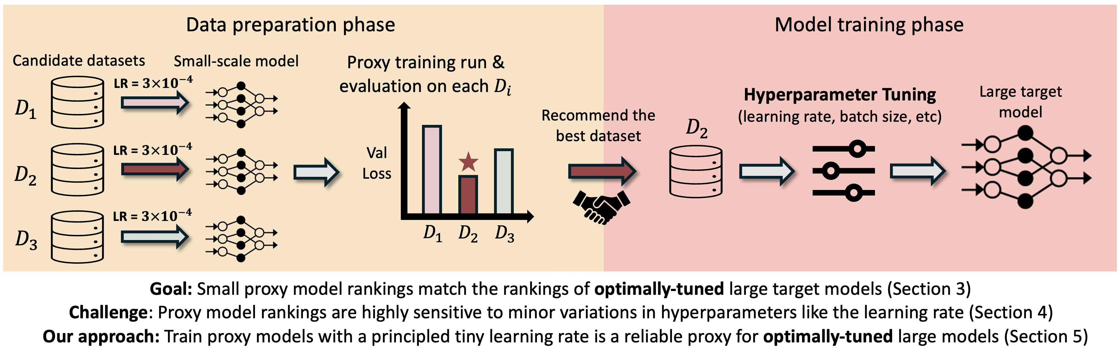
Rethinking data recipe ablation in practical workflows. Given the critical importance of data quality, modern AI development teams typically employ a division of labor: specialized data teams curate and optimize training data recipe, then recommend a high-quality dataset to model training teams who subsequently optimize training configurations (e.g., hyperparameters) specifically for the dataset (Figure 1). However, existing data-centric research evaluates and compares data recipes in ways fundamentally disconnected from this practical workflow. Most experiments in the data-centric literature and benchmarks evaluate all candidate data recipes under fixed training hyperparameters for “fairness”, while practical model training uses optimally-tuned hyperparameter configurations specifically adapted to each dataset. We therefore propose a refined objective for data-centric AI: find the data recipe that maximizes performance under optimally-tuned hyperparameters, reflecting how data is actually used in practice.

Minor variations in proxy training configuration can alter data recipe rankings (Section 12). The refined objective imposes a critical requirement for proxy-model-based techniques to succeed: the best data recipe identified through small-scale training runs must remain superior after (i) scaling the model to its target size and (ii) the training team optimizes training hyperparameters. However, this goal presents significant challenges given current proxy-model-based methods, where small proxy models evaluate and rank candidate datasets under a fixed, heuristically chosen hyperparameter configuration. Due to the strong interdependence between training hyperparameters and data distribution, each data recipe inherently requires its own optimal training configuration . If a dataset ordering collapses under such minor hyperparameter tweaks at the same proxy scale, broader sweeps at larger scales will almost certainly reorder the ranking further.

Training proxy models with tiny learning rates: a theoretically-grounded patch (Section 13). In the long run, the tight interplay between data and training hyperparameters suggests that these two components should be optimized jointly rather than tuned in separate, sequential steps. In the meantime, however, practitioners still need a drop-in patch that allows data teams to assess and optimize their data curation pipelines through small-scale experiments alone. We propose a simple yet effective remedy: train the proxy model with a tiny learning rate. Two key empirical observations inspire this approach: (i) within the same model architecture, datasets’ performance under a tiny learning rate strongly correlates with their optimal achievable performance after dataset-specific hyperparameter tuning; (ii) data recipe rankings remain stable under tiny learning rates as models scale from small to large sizes. We provide formal proof for these empirical findings for random feature models. Specifically, we prove that, as network width grows, training with a sufficiently small learning rate preserves the ordering of datasets, and the rankings converge to the ordering of their best achievable performance in the infinite-width limit. We further characterize this tiny learning rate regime through both theory and practical heuristics.

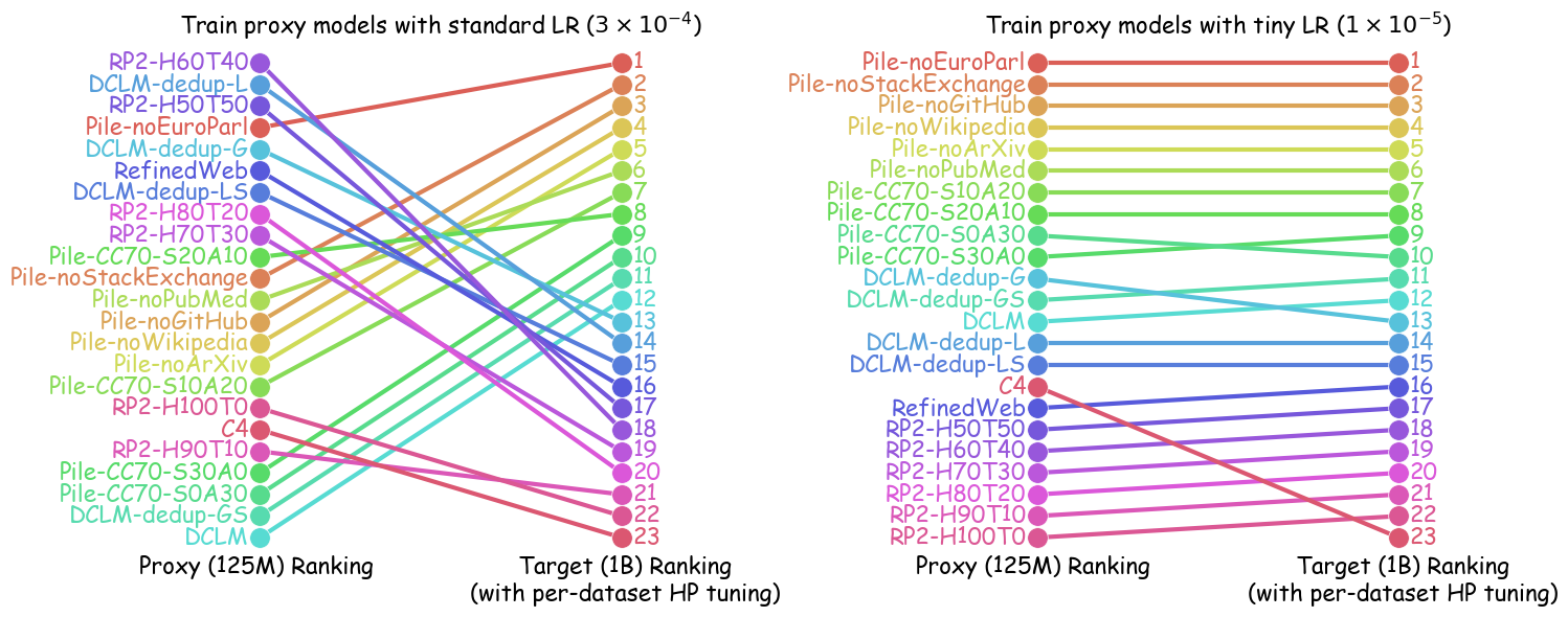
Experiments. We empirically evaluate the effectiveness of the tiny-learning-rate strategy through comprehensive experiments spanning multiple architectures, scales, and data curation scenarios. Our results demonstrate that proxy models trained with small learning rates achieve significantly improved transferability to hyperparameter-tuned larger target models. Figure 2 illustrates this improvement: the Spearman rank correlation for data recipe rankings between GPT2-125M and Pythia-1B improved to $`>0.95`$ across $`{23 \choose 2} = 253`$ data recipe pairs when using a tiny learning rate ($`10^{-5}`$) to train GPT2 instead of a commonly used learning rate ($`3 \times 10^{-4}`$).

Background: Guiding Data Curation with Small Proxy Models

In this section, we formalize the problem of data recipe ablation for large-scale model training.

Setup & Notations. Consider a target model architecture $`\theta_{\mathrm{tgt}}`$ and a pool of candidate datasets $`\mathcal{D}= \{D_1, D_2, \ldots, D_n\}`$, where each dataset results from a different data recipe (e.g., different curation algorithms, filter thresholds, or domain mixing ratios). Data recipe ablation aims to identify the optimal dataset $`D_{i^*} \in \mathcal{D}`$ that maximizes model performance on a validation set $`D_{\mathrm{val}}`$. Given a loss function $`\ell`$, let $`\ell_{\mathrm{val}}(\theta) := \ell(\theta; D_{\mathrm{val}})`$ denote the validation loss of model $`\theta`$. Since model performance depends critically on both training data and hyperparameters (e.g., learning rate, batch size), we write the trained model as $`\theta(D; \lambda)`$ for dataset $`D`$ and hyperparameter configuration $`\lambda`$.¹

Current practice of data recipe ablation with small proxy models. Directly evaluating candidate datasets by training a large target model on each is typically computationally prohibitive. A common practice to mitigate this issue involves using smaller “proxy models" ($`|\mathcal{M}_{\text{proxy}}| \ll |\mathcal{M}_{\text{target}}|`$) to predict data quality and determine which data curation recipe to use in large-scale training runs. Small models enable repeated training at substantially reduced computational costs, making them popular for ablation studies of various data curation pipelines . Current practices typically train proxy models on each $`D_i`$ (or its subset) using a fixed hyperparameter configuration $`\lambda_0`$, then rank the datasets based on small models’ performance $`\ell_{\text{val}}(\mathcal{M}_{\text{proxy}}(D_i; \lambda_0))`$.

Rethinking “High-quality Dataset": A Practical Development Perspective

Despite the broad adoption of small proxy models for data recipe ablation, the research community has a limited understanding of the conditions under which conclusions from small-scale experiments can be reliably transferred to large-scale production training. Before delving into the question of whether datasets that appear superior for small model training remain optimal for larger models, we must first establish a principled objective for data quality assessment. That is, what constitutes a “high-quality dataset" in practical model development? In this section, we discuss a subtle yet critical disconnect between practical workflows and the standard evaluation protocol in data-centric research.

Data recipes need to be assessed under individually optimized training configurations. In the existing literature (e.g., ), the effectiveness of data-centric algorithms is typically assessed by training a large target model on the curated dataset with a fixed set of hyperparameters. However, in the actual AI development pipelines, hyperparameter tuning will be performed, and the hyperparameters are tailored to the curated dataset. For instance, GPT-3 determines the batch size based on the gradient noise scale (GNS) , a data-specific statistic. Similarly, learning rates and optimization algorithms are usually adjusted in a data-dependent way. Therefore, we argue that a more reasonable goal for the data recipe ablation should optimize the selected dataset’s performance under hyperparameters tuned specifically for that dataset. This refined objective acknowledges the strong interaction between data and training hyperparameters in model training , emphasizing that data curation strategies should optimize for the training data’s optimally achievable performance rather than performance under a predefined, potentially suboptimal hyperparameter configuration. Formally, we formalize the data recipe ablation problem as $`D_{i^*} := \argmin_{i \in [n]} \min_{\lambda \in \Lambda} \ell_{\mathrm{val}}(\theta(D_i; \lambda))`$, where $`\Lambda`$ is a predefined feasible space of hyperparameters constrained by factors such as the available compute budget.

Proxy-Model Fragility under Hyperparameter Variation

Given our refined objective of identifying the dataset that performs best under its own optimized hyperparameters, we now examine whether current proxy-model practices align with this goal. Standard practice evaluates each candidate dataset by training a proxy model with a single, heuristically chosen hyperparameter configuration. Our investigation reveals a concerning consequence: even minor adjustments to the learning rate can flip the conclusions drawn from small proxy training runs. Consequently, the current practices can fail to identify datasets with the highest potential even for the same proxy model, and are even more likely to select suboptimal datasets when scaled to larger models with proper hyperparameter tuning.

Experiments: Learning rate sensitivity can undermine proxy models’ reliability. We investigate how minor variations in learning rate values can flip the conclusions drawn from small-scale experiments. Figure [fig:fragility] demonstrates this fragility by comparing DCLM with one of its variants that underwent more stringent deduplication (detailed configurations in Appendix 23.1.4).

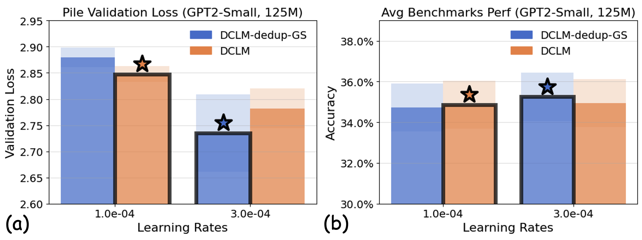
We train GPT2-Small (125M) on each dataset using two similar learning rates that reflect typical choices made by practitioners . The results reveal that dataset rankings can be inconsistent with respect to the chosen learning rate. At a lower learning rate, DCLM is superior on both the validation loss and the downstream benchmarks. However, a slight increase in learning rate reverses this performance ranking. This reversal likely stems from DCLM’s relatively loose deduplication criteria, which tend to favor smaller learning rates, whereas its more stringently deduplicated variant performs better with larger learning rates. The sensitivity to learning rate selection highlights a critical limitation of small-scale proxy experiments: conclusions drawn from small-scale training runs with fixed configurations can overfit to those specific settings, potentially leading to suboptimal data curation decisions when scaling to large-scale model training.

High-level intuition: The curse of higher-order effects. To gain intuition about why different learning rates lead to inconsistent data recipe rankings in proxy models, we consider a highly simplified one-step gradient descent setting, where the change in validation loss $`\ell_{\mathrm{val}}`$ after one gradient update can be approximated through Taylor expansion:

\begin{align*}
\Delta \ell_{\mathrm{val}}(\theta) 
= \ell_{\mathrm{val}}(\theta- \eta \nabla \ell(\theta)) - \ell_{\mathrm{val}}(\theta) 
\approx -\eta \nabla \ell_{\mathrm{val}}(\theta) \cdot \nabla \ell(\theta) + \frac{\eta^2}{2} \nabla \ell(\theta)^T H_{\ell_{\mathrm{val}}}(\theta) \nabla \ell(\theta)
\end{align*}

where $`H_{\ell_{\mathrm{val}}}`$ is the Hessian of the validation loss. Consider two datasets $`D_i`$ and $`D_j`$ with corresponding training losses $`\ell_i`$ and $`\ell_j`$. When the learning rate is low, their ranking primarily depends on the first-order gradient alignment terms: $`\nabla \ell_{\mathrm{val}}(\theta) \cdot \nabla \ell_i(\theta)`$ versus $`\nabla \ell_{\mathrm{val}}(\theta) \cdot \nabla \ell_j(\theta)`$. However, at moderate learning rates, the second-order term becomes significant. For example, two datasets $`D_i`$ and $`D_j`$ that have better first-order gradient alignment can reverse their ordering once the quadratic terms outweigh this difference at moderate values of $`\eta`$. Overall, the ranking flip can occur as the learning rate moves beyond the tiny regime, where the higher-order curvature term can dominate the change in the loss, override first-order alignment, and ultimately flip the dataset rankings.

Training small proxy models with tiny learning rates improves transferability to tuned target models

To reduce hyperparameter sensitivity in data recipe ablation and better align with the practical goal of identifying the recipe with the highest performance potential, one straightforward approach is to sweep through extensive hyperparameter configurations for each candidate data recipe and compare their optimal validation loss across all settings. However, this requires numerous training runs per candidate data recipe, which can be prohibitively expensive even with smaller proxy models. Moreover, training randomness can introduce significant variance in results, further reducing the reliability of such comparisons. Building on insights from our one-step gradient update analysis, we propose a simple yet effective solution: train proxy models with very small learning rates and rank data recipes by their validation losses under this regime.

Empirical Findings & High-level Intuition

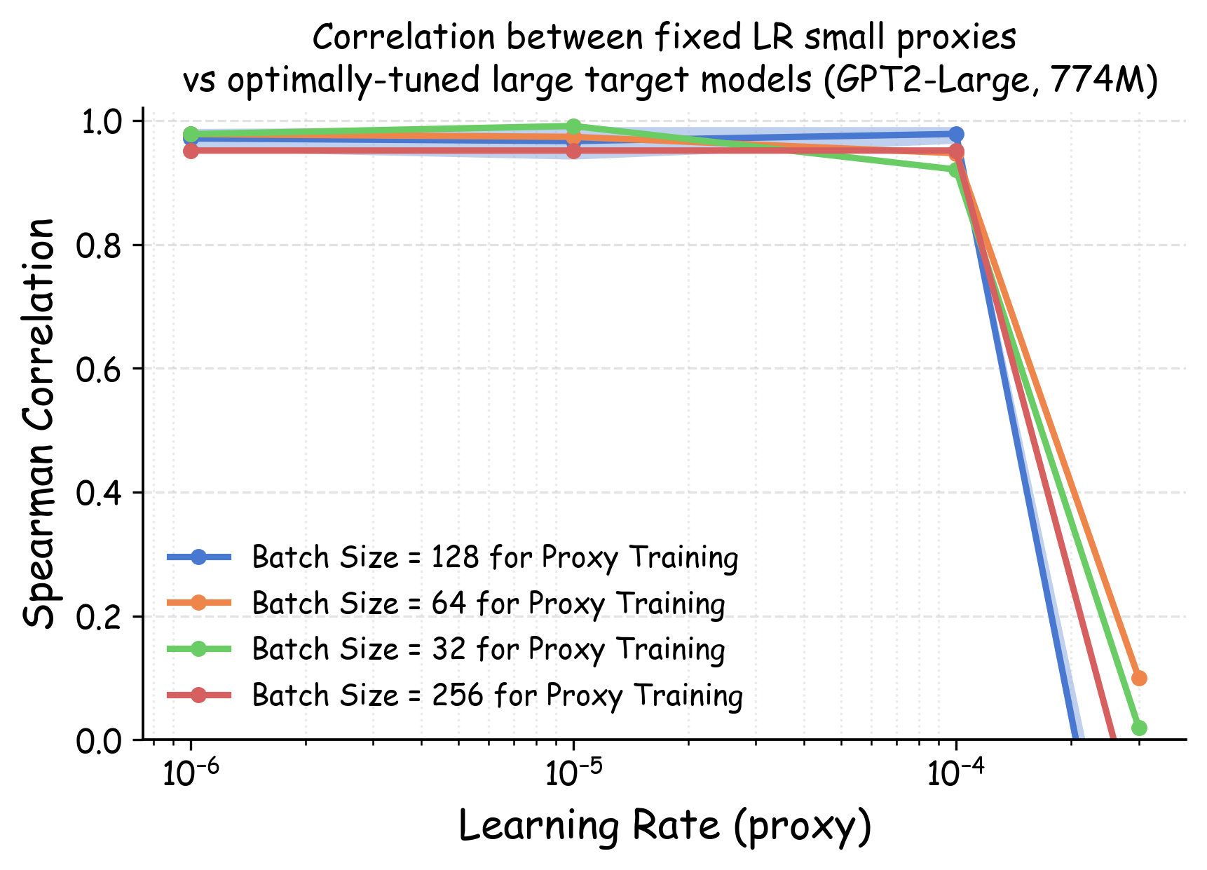
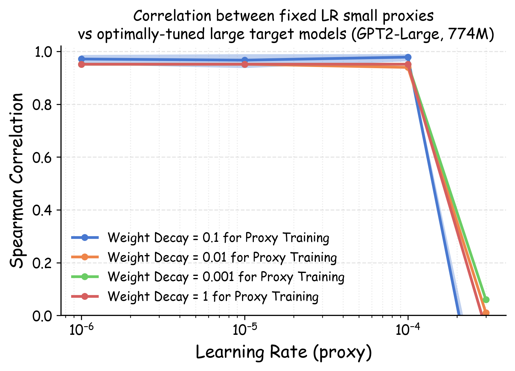
Notations. We denote the optimal validation loss achievable for a dataset $`D`$ by $`\ell_{\text{val-opt}}(\theta(D)) = \min_{\eta \in \Lambda} \ell_{\mathrm{val}}(\theta(D; \eta))`$ where the minimum is taken over the full hyper-parameter space $`\Lambda`$. In our experiment, this optimum is approximated via a wide range of hyperparameter sweeps. Our pilot study (see Section 14 and Appendix 23) shows that dataset rankings are most sensitive to the learning rate, while relatively stable across other major hyperparameters such as batch size. Therefore, throughout this section, we simplify notation and write $`\theta(D; \eta)`$ to denote a model trained with learning rate $`\eta`$ while all other hyperparameters are fixed to standard values from prior literature (details in Appendix 23). Given two datasets $`D_i`$ and $`D_j`$, we denote by $`\Delta\ell_{\mathrm{val}}^{(i, j)}(\theta, \eta)`$ the difference in validation loss when a model $`\theta`$ is trained on these datasets using a fixed learning rate $`\eta`$, and by $`\Delta\ell_{\text{val-opt}}^{(i, j)}(\theta)`$ the difference in their optimal validation losses after full hyperparameter tuning:

\begin{align*}
\Delta\ell_{\mathrm{val}}^{(i, j)}(\theta, \eta) = \ell_{\mathrm{val}}(\theta(D_i; \eta)) - \ell_{\mathrm{val}}(\theta(D_j; \eta)), ~~~\Delta\ell_{\text{val-opt}}^{(i, j)}(\theta) = \ell_{\text{val-opt}}(\theta(D_i)) - \ell_{\text{val-opt}}(\theta(D_j))
\end{align*}

Our objective is to identify a specific learning rate $`\eta_0`$ for proxy models that reliably preserves the ranking of datasets based on their fully-optimized performance on large target models:

\begin{align}
\sign(\Delta\ell_{\mathrm{val}}^{(i, j)}(\theta_{\mathrm{proxy}}, \eta_0)) = \sign(\Delta\ell_{\text{val-opt}}^{(i, j)}(\theta_{\mathrm{tgt}}))
  \label{eq:transfer-goal}
\end{align}

We present two key empirical findings (settings detailed in Appendix 23) and the high-level intuition behind them, which motivates our solution of training proxy models with tiny learning rates.

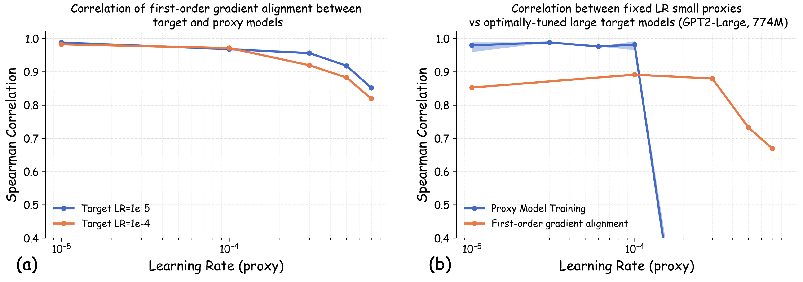
Finding I: For the same model, tiny learning rate performance correlates with optimal hyperparameter-tuned performance. We first investigate the correlation between the losses for the same model architectures trained by different learning rates. Figure 3(a) shows the correlation between GPT2-Small’s validation loss on the Pile validation split when trained with a tiny learning rate versus its minimum validation loss achieved through extensive hyperparameter sweeps, evaluated across 23 data recipes. The strong correlation demonstrates that for a given model architecture, training with a tiny learning rate provides a reliable proxy for optimized performance after full hyperparameter tuning. The relative utility of datasets, as measured by tiny learning rate training, is preserved when the same model is optimally configured. Formally, for small $`\eta_0`$, we observe that

\begin{align}
\sign(\Delta\ell_{\mathrm{val}}^{(i, j)}(\theta_{\mathrm{proxy}}, \eta_0)) = \sign(\Delta\ell_{\text{val-opt}}^{(i, j)}(\theta_{\mathrm{proxy}}))
\label{eq:transfer-samescale}
\end{align}

for most dataset pairs $`(D_i, D_j)`$. Intuition: In one-step gradient update, when the learning rate $`\eta \rightarrow 0`$, model updates are dominated by the first-order gradient alignment term $`\nabla \ell_{\mathrm{val}}(\theta) \cdot \nabla \ell(\theta)`$. This alignment measures the distributional similarity between training and validation datasets from the neural network’s perspective, and is a metric widely used in data selection literature . Therefore, the validation loss at an infinitesimal learning rate effectively upper-bounds the irreducible train–validation distribution gap, and its ranking across datasets is strongly correlated with the best loss each dataset can achieve after full hyperparameter tuning.

Finding II: Dataset rankings remain consistent across model scales when both use tiny learning rates. In Figure 3(b), we visualize the heatmap of Spearman rank correlation coefficients between proxy and target model dataset rankings across various learning rate combinations. The lower-left region of the heatmap shows that when both proxy and target models are trained with tiny learning rates, the cross-scale transferability of dataset rankings achieves nearly perfect correlation. Formally, this suggests that when both $`\eta_0`$ and $`\eta_1`$ are small, we have

\begin{align}
\sign(\Delta\ell_{\mathrm{val}}^{(i, j)}(\theta_{\mathrm{proxy}}, \eta_0)) = \sign(\Delta\ell_{\mathrm{val}}^{(i, j)}(\theta_{\mathrm{tgt}}, \eta_1))
\label{eq:transfer-crossscale}
\end{align}

for most dataset pairs $`(D_i, D_j)`$. Intuition: While gradient alignment (the first-order term) is still model-dependent, its relative ranking across different candidate datasets tends to be preserved across model architectures . When both proxy and target models operate in the tiny-LR regime, their loss rankings are primarily determined by the distributional similarity between training and validation data. As a result, the validation-loss orderings remain relatively stable across different model scales, despite their differing capacities.

Collectively, the empirical observations in ([eq:transfer-samescale]) and ([eq:transfer-crossscale]) together lead to ([eq:transfer-goal]) when using a small learning rate, motivating our strategy of ranking datasets by their tiny‑LR losses on proxy models.

Theoretical Analysis

We choose the random feature model because it is one of the simplest models whose training dynamics at different learning rates and scales can be approximately characterized mathematically. As the training dynamics of deep neural networks are usually non-tractable, a series of recent works have used random feature models as proxies to understand the dynamics of neural networks under model scaling . The random feature model is also closely related to the Neural Tangent Kernel (NTK), a key concept in the theory of deep neural networks that has often yielded valuable insights for developing data-centric techniques .

Interpretation.

Intuition & Proof sketch. Similar to our intuition from one-step gradient update, our analysis of random feature models decomposes the change in validation loss under SGD into a deterministic drift term that captures the true quality gap between datasets and a variance term from stochastic updates. When a sufficiently wide model is trained with a small learning rate, the drift dominates the variance, so the observed sign of the loss difference matches the sign of the infinite-width optimum gap with high probability. This formalizes the intuition that small learning rates suppress the curse of higher-order effects that otherwise scramble rankings.

An Empirical Characterization of “Tiny” Learning Rates

Our analysis suggests the potential benefits of training proxy models with tiny learning rates. A natural question is how small should the learning rate be for reliable proxy training runs? We provide both theoretical guidance and practical recommendations, with extended discussion in Appendix 22.

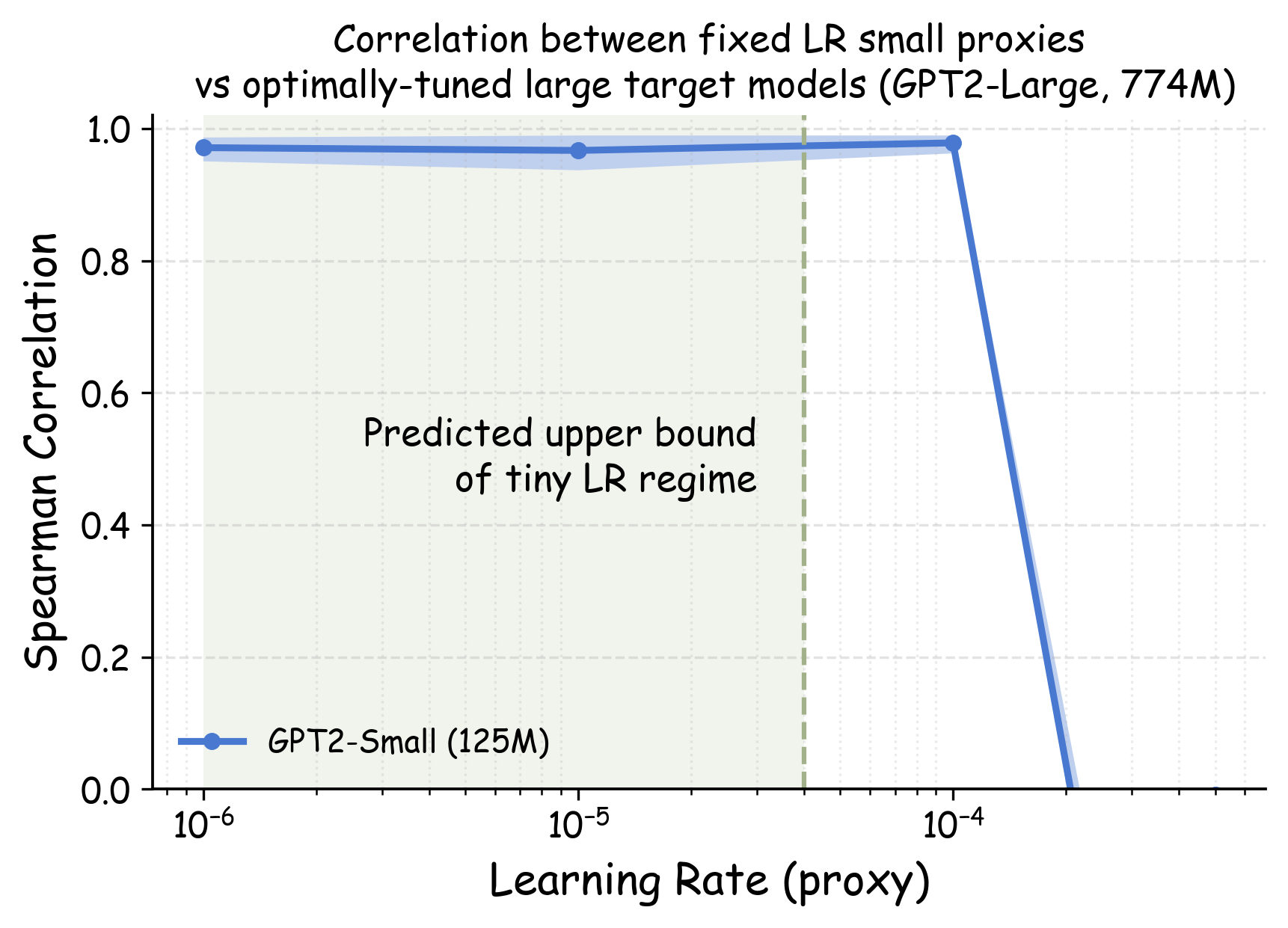
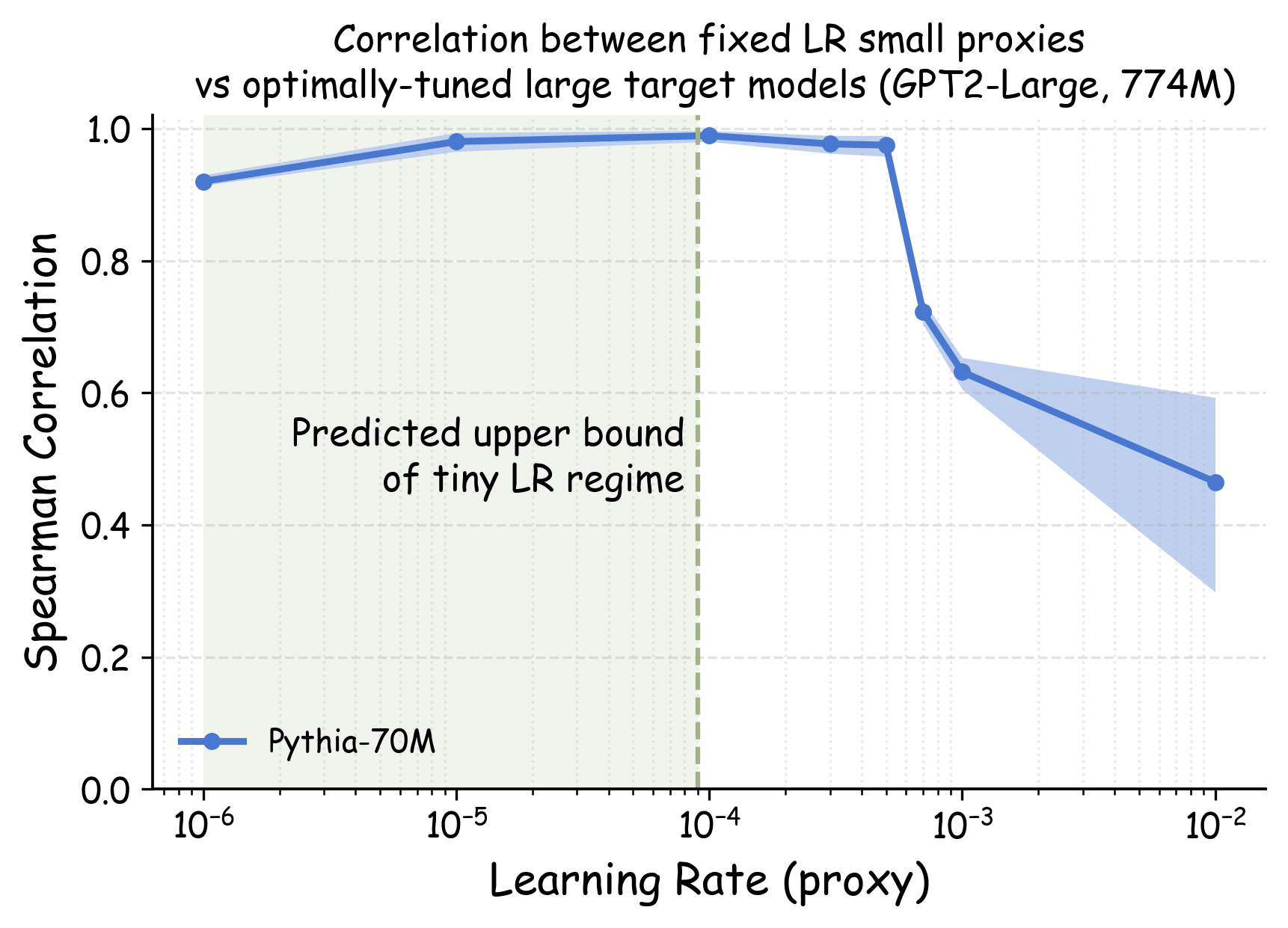
Theoretical guidance. Our theoretical analysis (detailed in Appendix 22) establishes an upper bound for what constitutes a “tiny" learning rate in the context of one-step mini-batch SGD. At a high level, we show that $`\etatiny`$ needs to be far smaller than $`1/\lambda_{\max}`$, where $`\lambda_{\max}`$ is the top eigenvalue of the validation loss Hessian. We stress that one-step analysis has often been shown to give quantitatively useful guidance when coupled with empirical validation (e.g. ). Following the established precedent, we treat our derived bound as principled guidance rather than as a rigid constraint. In Appendix 22, we use model checkpoints that have undergone short warmup training to estimate $`\etatiny`$’s upper bound, and we show that these theoretically-predicted values consistently fall within the empirically-identified regime of learning rates with high transferability.

Choosing $`\etatiny`$ in practice: a simple rule of thumb. While estimating $`\etatiny`$ from proxy model checkpoints is computationally inexpensive, we find that a simpler heuristic suffices for most LLM pretraining scenarios. In Appendix 22, we discuss the relationship between $`\etatiny`$ and the standard learning rate for language model pretraining. Empirically, we find that using learning rates 1-2 orders of magnitude smaller than standard choices of learning rates generally works well. For language model pretraining, this typically translates to learning rates of approximately $`10^{-5}`$ to $`10^{-6}`$. In Section 14.2, we will see that these values work consistently well across various model scales.

Practical implementation also requires consideration of the lower bounds of $`\etatiny`$ due to numerical precision. However, we find that the recommended range of $`10^{-5}`$ to $`10^{-6}`$ lies comfortably above the threshold where numerical errors become significant in standard training. Our experiments confirm that learning rates in this range maintain numerical stability while achieving the desired transferability properties. We provide additional analysis of numerical considerations in Appendix 22.

Experiments

Experiment Settings

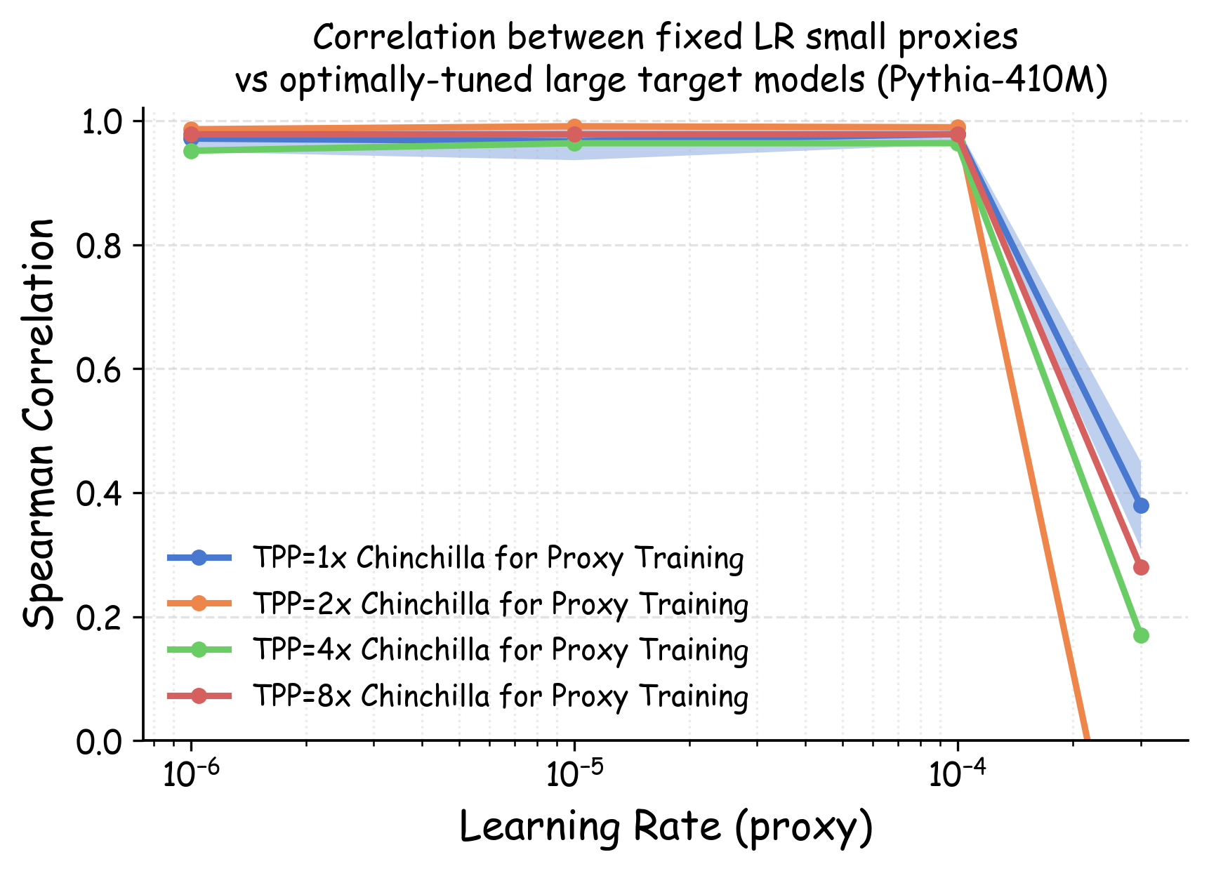
Evaluation protocol. We conduct comprehensive evaluations across multiple model architectures (GPT2, Pythia, OPT) spanning sizes from 70M to 1B parameters. We assess transferability using both the validation loss across diverse domains from The Pile corpus and downstream benchmark performance on HellaSwag, Winogrande, OpenBookQA, ARC-Easy, and CommonsenseQA. Following standard practices, we primarily set the token-per-parameter ratio to 20, adhering to Chinchilla’s compute-optimal ratio . Additional ablation studies examining overtraining scenarios (with ratios up to 160) are presented in Appendix 23.2.2.

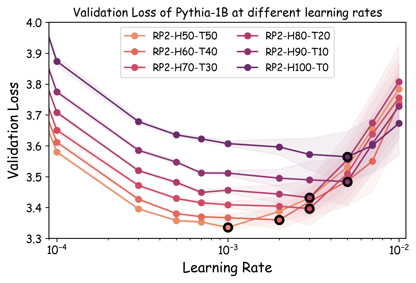
Data Recipes. To comprehensively evaluate proxy model transferability across the diverse data curation decisions faced in production scenarios, we construct 23 data recipes spanning four critical dimensions of language data curation. (1) Domain composition and ablation. We create 10 domain mixture variations from The Pile . Specifically, 4 recipes maintain a fixed 70% Pile-CC allocation while varying the remaining 30% between StackExchange and ArXiv. Additionally, 6 recipes are created by excluding one domain from the full Pile dataset to assess domain importance. (2) Existing dataset comparison. We evaluate 3 widely-adopted pretraining corpora: C4 , DCLM-baseline , and RefinedWeb . They all originate from Common Crawl but vary in curation strategies such as data filtering criteria and deduplication algorithms. (3) Scoring-based data filter. We construct 6 data recipes using different mixing ratios of head-middle versus tail partitions from RedPajama-V2 , ranging from 50:50 to 100:0. These partitions are defined by the perplexity scores from a 5-gram Kneser-Ney model trained on Wikipedia . (4) Deduplication. We create 4 variants of DCLM-baseline by modifying the stringency of Massive Web Repetition Filters , adjusting n-gram and line/paragraph repetition thresholds. The detailed description for the data recipes considered in this work is summarized in Appendix 23.1.4 and Table [table:dataset-recipes].

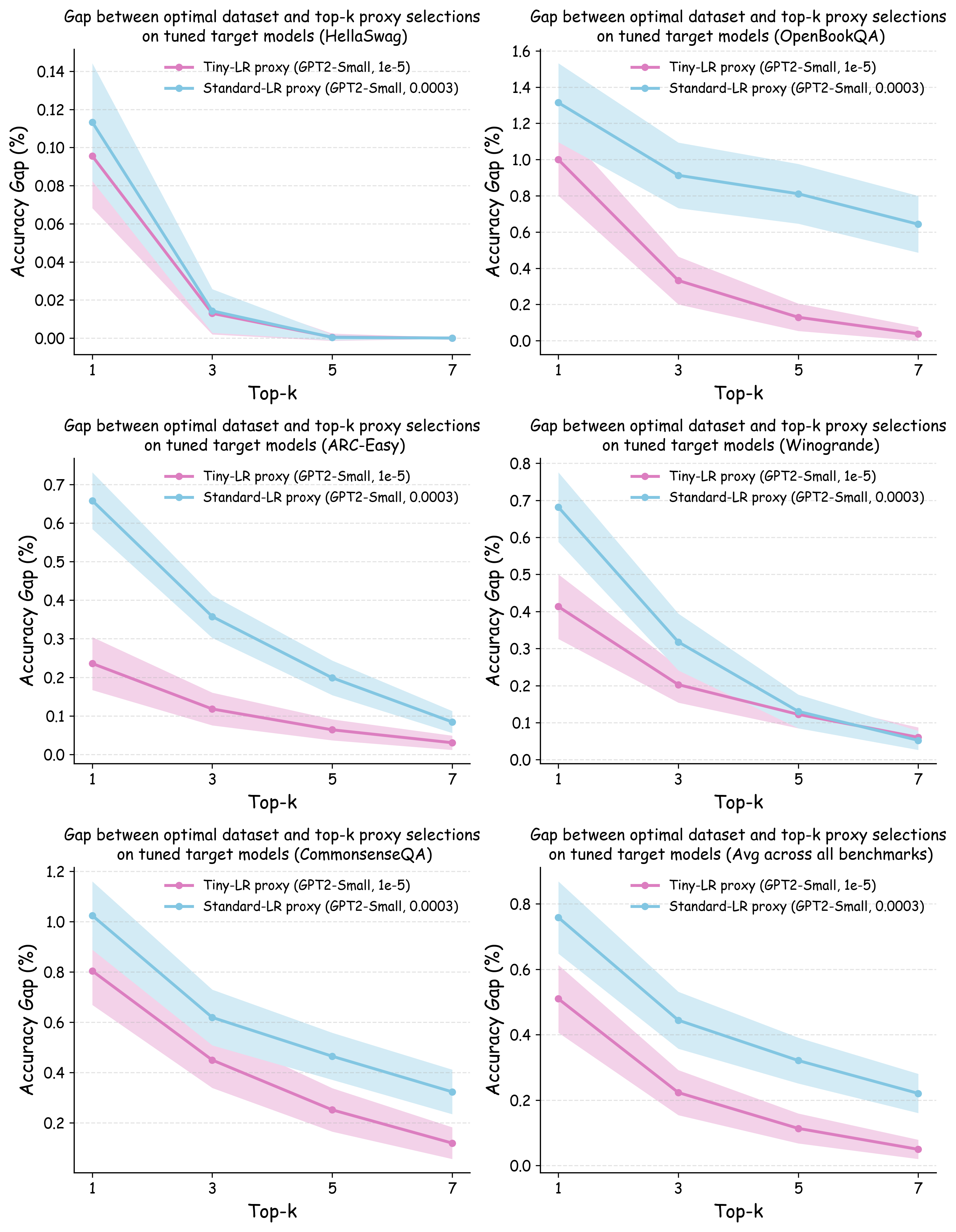
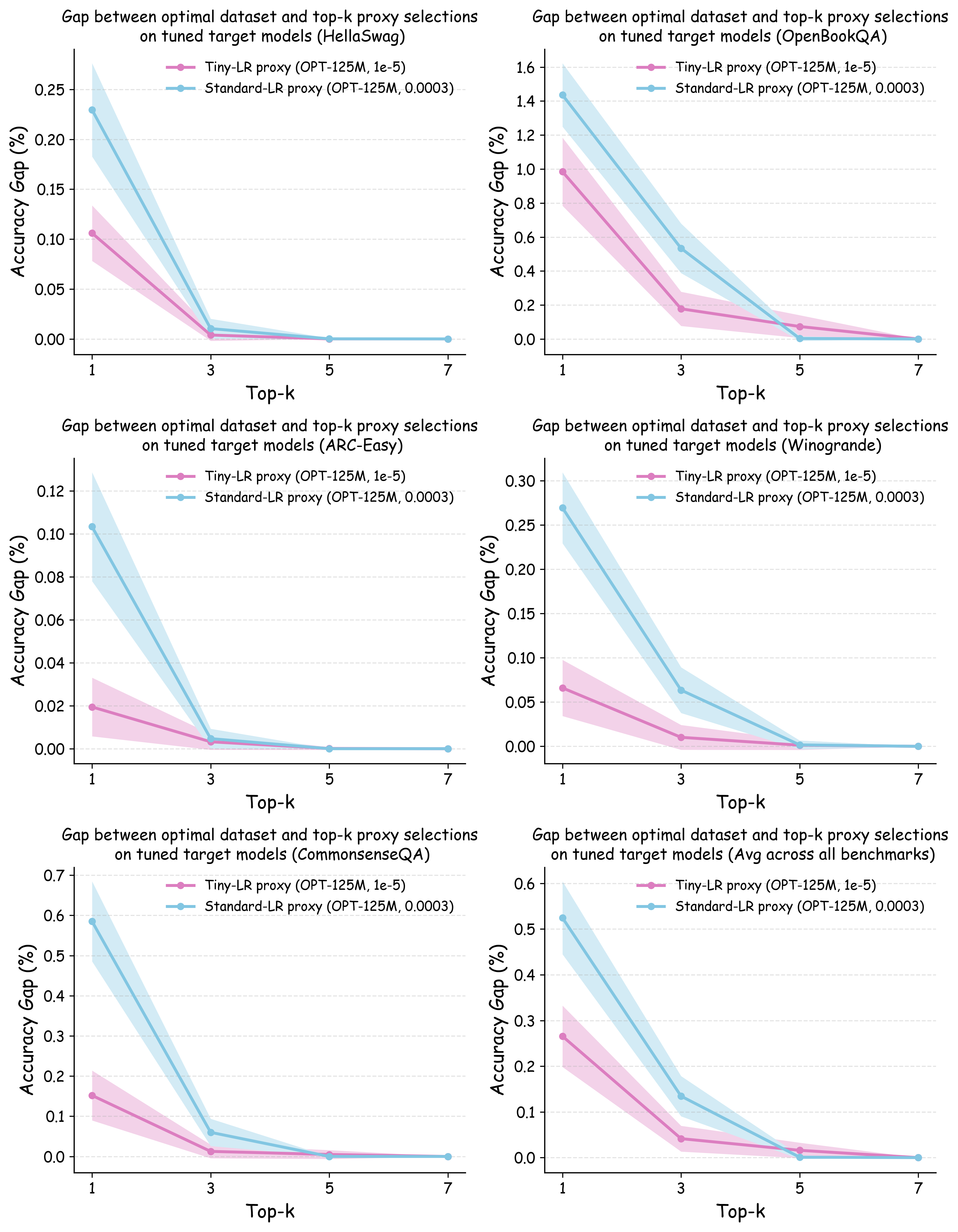
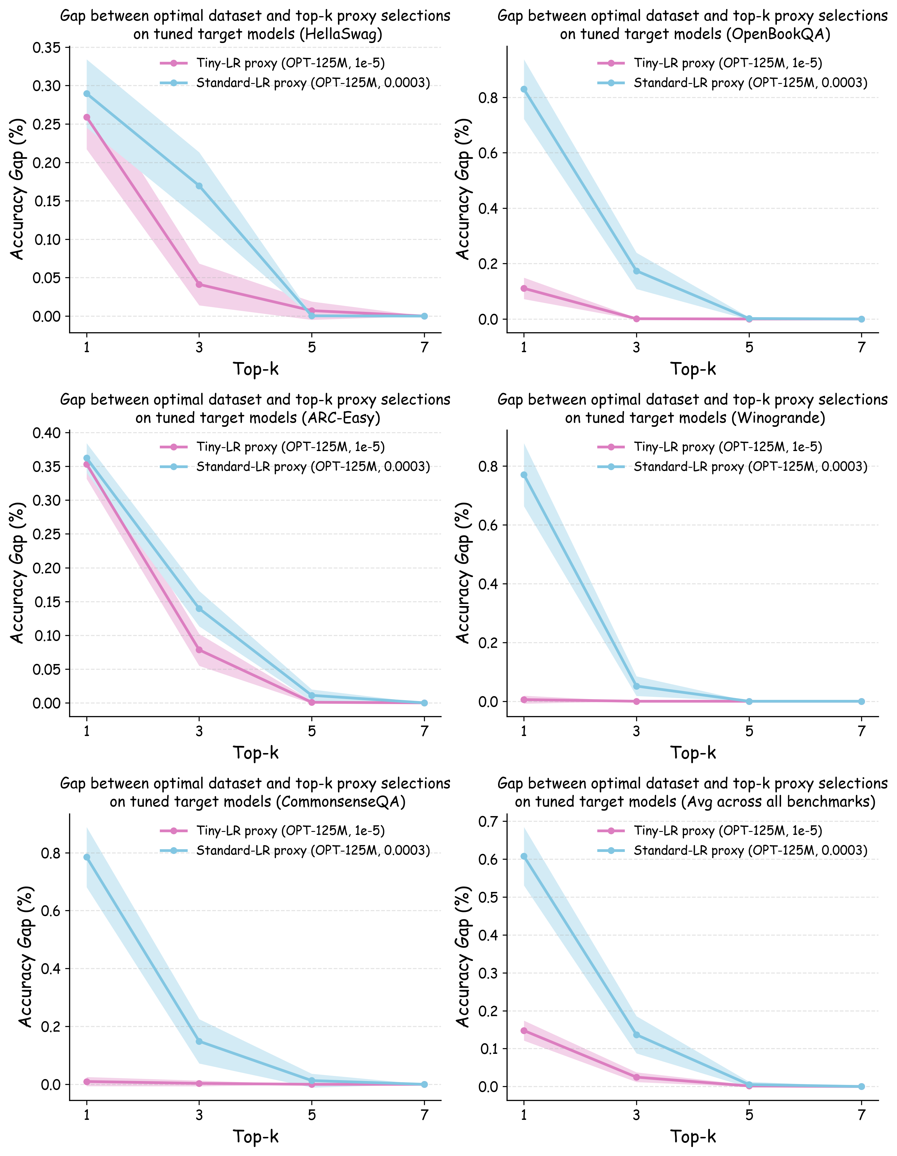
Evaluation Metrics. We report two complementary quantities that capture (i) rank fidelity and (ii) practical decision risk. Spearman rank correlation. This measures the monotone agreement between the proxy-induced ranking and the target-scale ranking, where the target ranking is obtained by training the target model on each dataset with its own tuned hyperparameters. Top-$`k`$ Decision Regret. This addresses the practical question: if a data team selects the top-$`k`$ data recipes ranked by the proxy model for full-scale evaluation, how suboptimal might their final choice be compared with the best data recipe? Formally, we compute the performance difference between the truly optimal dataset and the best-performing dataset among the proxy’s top-$`k`$ selections, with both datasets evaluated using their individually optimized hyperparameters on the target model.

Due to space constraints, we leave detailed model training and other settings to Appendix 23.1.

Results

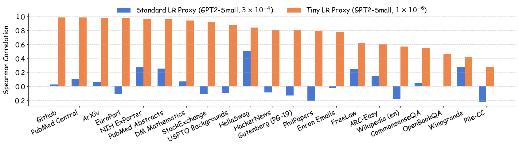
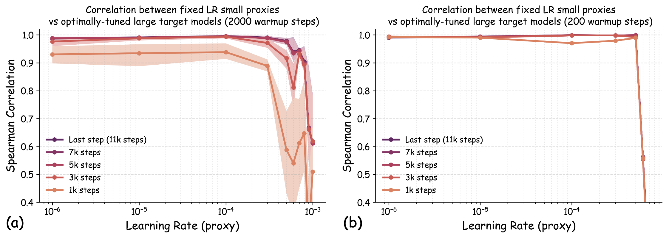
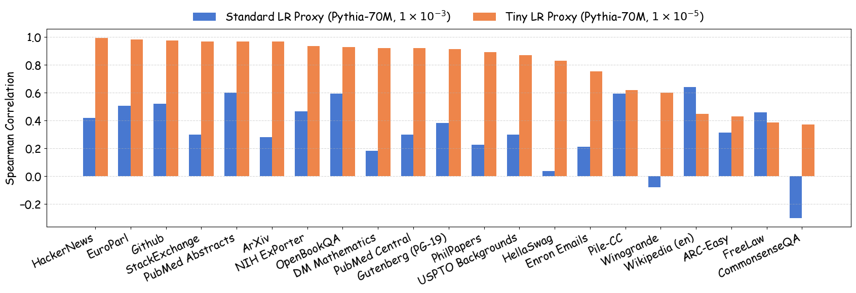
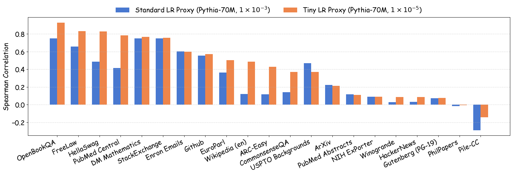
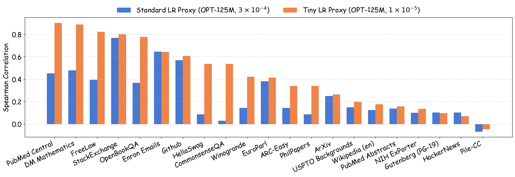
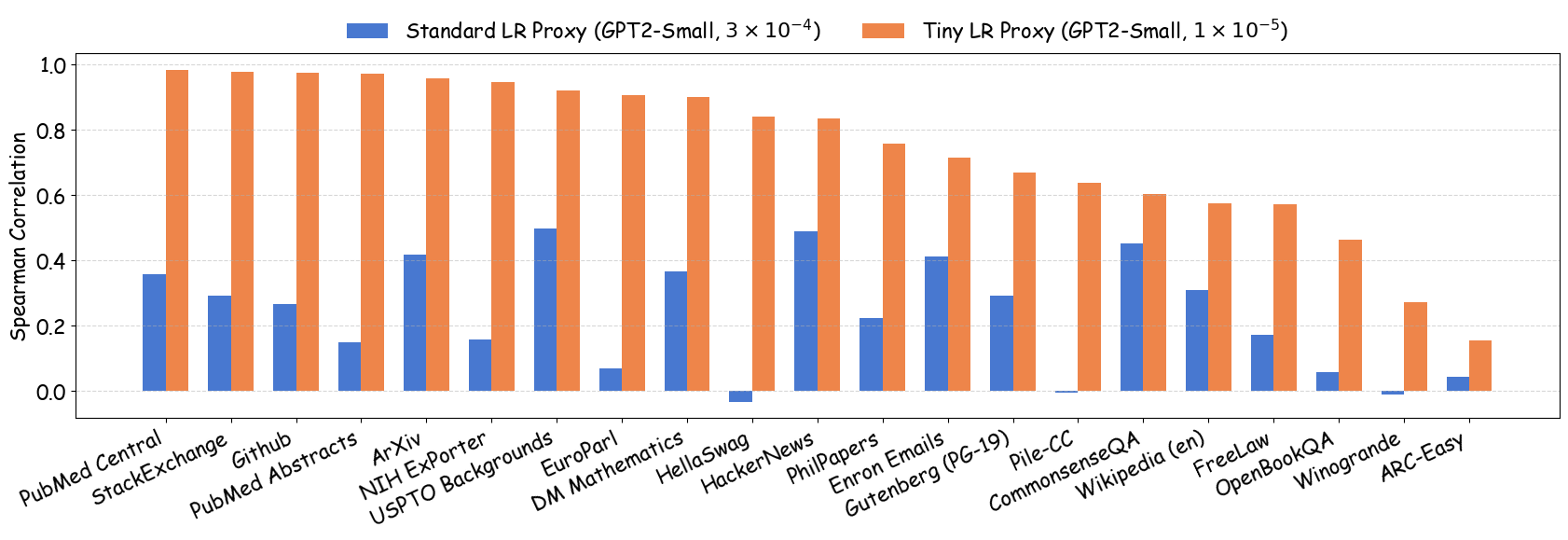
As shown in Figure 5 (a), training proxy models with standard learning rates ($`3 \times 10^{-4}`$ for GPT2-Small and OPT-125M , $`10^{-3}`$ for Pythia-70M ) yields only modest ranking agreement, with Spearman rank correlation $`\rho < 0.75`$. This poor rank consistency can lead to suboptimal data selection decisions and performance degradation in large-scale model training. However, when the learning rate drops below $`1 \times 10^{-4}`$, we observe substantial improvements in ranking agreement. Under these smaller learning rates, the proxy models achieve performance ranking correlations above 0.92 across all three architectures. Figure 4 extends these results beyond aggregated validation loss to examine how small learning rates affect the reliability of proxy models across individual Pile domains and downstream benchmarks. The results demonstrate that training proxy models with reduced learning rates improves data recipe ranking correlations across nearly all evaluation metrics. In contrast, standard learning rate proxies exhibit catastrophic failure across most metrics, yielding near-zero or negative correlations in many domains.

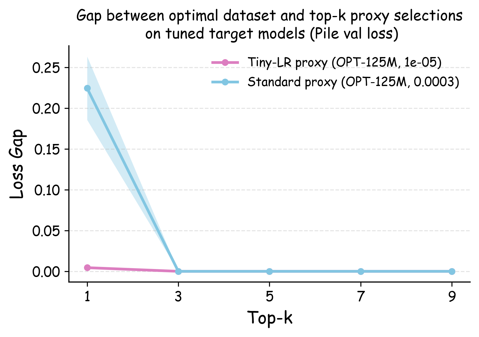
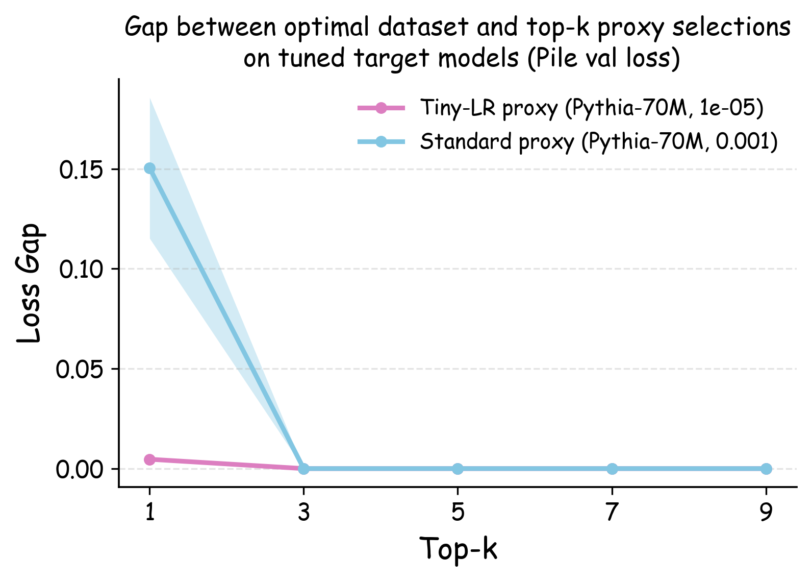
Figure 5 (b) and (c) demonstrate the practical implications of these ranking correlations through the top-$`k`$ decision regret metric. When data teams select the top-$`k`$ data recipes for large-scale model training based on small-scale experiments, proxies trained with tiny learning rates consistently minimize the performance gap relative to the ground-truth optimal data recipes for the target model. In contrast, standard learning rate proxies can incur $`> 0.25`$ validation loss degradation when $`k`$ is small. This stark difference demonstrates that conducting small-scale ablation studies with smaller learning rates can significantly enhance the reliability of data decisions in large-scale model training.

Conclusion & Future Works

We demonstrate that standard data recipe ablations are brittle in small-scale settings; even slight adjustments to the learning rate can yield inconsistent findings. To address this, we proposed a simple yet effective solution: using tiny learning rates during proxy model training. In the following, we discuss the scope of this work and outline several potential future directions.

Joint optimization of data and training configurations. As we mentioned in the Introduction, our approach serves as a simple remedy to the proxy-model-based approach. However, because the challenge stems from the strong coupling between training configurations and datasets, we argue that, in the long term, datasets and tunable training configurations should be jointly optimized. Recent advances in gradient-based hyperparameter optimization and algorithm unrolling may provide inspiration and building blocks for this direction.

acknowledgement

This work is supported in part by the Apple PhD Fellowship. Ruoxi Jia and the ReDS lab acknowledge support through grants from the National Science Foundation under grants IIS-2312794, IIS-2313130, and OAC-2239622.

We thank Lin Chen, Mohammadhossein Bateni, Jennifer Brennan, Clayton Sanford, and Vahab Mirrokni at Google Research for their helpful feedback on the preliminary version of this work.

acknowledgement

This work is supported in part by the Apple PhD Fellowship. Ruoxi Jia and the ReDS lab acknowledge support through grants from the National Science Foundation under grants IIS-2312794, IIS-2313130, and OAC-2239622.

We thank Lin Chen, Mohammadhossein Bateni, Jennifer Brennan, Clayton Sanford, and Vahab Mirrokni at Google Research for their helpful feedback on the preliminary version of this work.

Theoretical Analysis

In this section, we analyze two-layer random feature networks and prove that the transferability to datasets’ minimum achievable performance holds when the proxy models are trained with tiny learning rates.

Setup

Random Feature Networks. We analyze two-layer random feature networks, also known as random feature models. Let $`\sigma : \reals \to \reals`$ be a Lipschitz function. The weights in the first layer $`\mU := (\vu_1, \dots, \vu_m) \in \R^{d \times m}`$ are drawn independently from a bounded distribution $`\cU`$ on $`\R^d`$. For all $`\vx`$ in a compact input space $`\cX \subseteq \R^d`$, define the feature map

\begin{align}
\phi^{(\mU)}_i(\vx) = \sigma(\inne{\vu_i}{\vx}), \qquad \phi^{(\mU)}(\vx) = (\phi^{(\mU)}_1(\vx), \dots, \phi^{(\mU)}_m(\vx))^{\top} \in \reals^{m}.
\end{align}

The second layer is parameterized by a weight vector $`\vtheta \in \R^m`$. Given the first-layer weights $`\mU`$ and the second-layer weights $`\vtheta`$, the two-layer network outputs

\begin{align}
    f^{(\mU)}_{\vtheta}(\vx) = \frac{1}{\sqrt{m}} \inne{\vtheta}{\phi^{(\mU)}(\vx)}.
\end{align}

This function computes a linear combination of randomly generated nonlinear features of the input $`\vx`$.

Data Distribution. A data distribution $`D`$ is a probability distribution over $`\cX \times \reals`$, where the marginal distribution on inputs $`\vx`$, denoted as $`\Dx`$, is assumed to admit a continuous density function over $`\cX`$. Each sample $`(\vx, y) \sim D`$ consists of an input $`\vx`$ and a label $`y`$. We say that $`D`$ has no label noise if there exists a target function $`f^*_D : \cX \to \reals`$ such that $`y = f^*_D(\vx)`$ almost surely for $`(\vx, y) \sim D`$.

Training. We define $`\cP_m(D; \eta, B, T)`$ as the distribution of $`(\vtheta, \mU)`$ of a width-$`m`$ network trained on a data distribution $`D`$ with the following procedure. Define the MSE loss as:

\begin{align}
    \ell(f; \vx, y) := \frac{1}{2}(f(\vx) - y)^2,
    \qquad
    \cL_{D}(\vtheta; \mU) = \cE_{(\vx,y) \sim D} \left[ \ell(f^{(\mU)}_{\vtheta}; \vx, y) \right].
\end{align}

We randomly sample the first-layer weights $`\mU \sim \cU^m`$ as described above and freeze them. We then optimize the second-layer weights $`\vtheta`$ using one-pass mini-batch SGD with batch size $`B`$ and learning rate $`\eta`$, starting from $`\vtheta_0 = \vzero`$. The update rule is given by:

\begin{align}
    \vtheta_{t+1} &= \vtheta_t - \frac{\eta}{B} \sum_{b=1}^{B} \left.\frac{\partial}{\partial \vtheta} \left(\ell(f^{(\mU)}_{\vtheta}; \vx_{t,b}, y_{t,b})\right)\right|_{\vtheta = \vtheta_t},
\end{align}

where $`(\vx_{t,b}, y_{t,b})`$ is the $`b`$-th training input and label in the $`t`$-th batch, sampled independently from $`D`$. $`\cPm(D; \eta, B, T)`$ is the distribution of $`(\vtheta_T, \mU)`$ obtained by running the above procedure for $`T`$ steps.

Validation. We fix a data distribution $`\Dval`$ for validation, called the validation distribution. The validation loss is given by

\begin{align}
    \cLval(f) = \cE_{(\vx,y) \sim \Dval} \left[ \ell(f; \vx, y) \right].
\end{align}

Given a training distribution $`D`$ with no label noise, we define the expected validation loss of a width-$`m`$ network trained on $`D`$ with batch size $`B`$ and learning rate $`\eta`$ for $`T`$ steps as

\begin{align}
    \cIvalm(D; \eta, B, T) = \E_{(\vtheta, \mU) \sim \cPm(D; \eta, B, T)} \left[ \cLval(f^{(\mU)}_{\vtheta}) \right].
\end{align}

Further, we define the best achievable validation loss of a width-$`m`$ network trained on $`D`$ with batch size $`B`$ for $`T`$ steps (after tuning the learning rate $`\eta`$) as

\begin{align}
    \cIvaloptm(D; B, T) &= \min_{\eta > 0}\left\{ \cIvalm(D; \eta, B, T) \right\}, \\
    \quad \etaopt^{(m)}(D; B, T) &= \argmin_{\eta > 0}\left\{ \cIvalm(D; \eta, B, T) \right\}.
\end{align}

Understanding the Infinite-Width Limit. Before stating our assumptions on the data distributions, we first provide some intuition on the infinite-width limit of the random feature model. A random feature model with width $`m`$ naturally induces a kernel function $`K^{(\mU)}(\vx, \vx') = \frac{1}{m} \langle \phi^{(\mU)}(\vx), \phi^{(\mU)}(\vx') \rangle`$ on the input space $`\cX`$. As $`m \to \infty`$, the randomness in the features $`\phi^{(\mU)}(\vx)`$ averages out due to the law of large numbers and the kernel $`K^{(\mU)}(\vx, \vx')`$ converges to a deterministic kernel $`K(\vx, \vx')`$:

\begin{align}
    K(\vx, \vx') = \E_{\vu \sim \cU}\left[ \sigma(\langle \vu, \vx \rangle)\sigma(\langle \vu, \vx' \rangle) \right].
\end{align}

In this limit, the kernel $`K`$ captures the expressive power of the infinite-width model: learning in this regime becomes equivalent to kernel regression using $`K`$. The function class defined by the model becomes a Reproducing Kernel Hilbert Space (RKHS) associated with $`K`$, denoted as $`\cH_K`$. The properties of this kernel—especially whether it is positive definite and how well it aligns with the target function—directly influence the learnability of the problem. With this in mind, we now formalize the assumptions we make about the data distributions in our theoretical analysis.

Well-Behaved Distributions. We say that a distribution $`D`$ with no label noise is well-behaved if the following conditions are satisfied:

1. Full Support on the Input Space. The probability density of $`\Dx`$ is strictly positive on the input space $`\cX`$. This ensures that $`\Dx`$ has full support on $`\cX`$.

2. Positive-Definite Kernel. The kernel $`K(\vx, \vx')`$ has strictly positive minimum eigenvalue on $`L^2(\Dx)`$, the square-integrable function space under $`\Dx`$. This prevents the kernel function from being degenerate.

3. Realizability at Infinite Width. The target function $`f^*_D`$ lies in the RKHS $`\cH_K`$ associated with the kernel $`K`$. More specifically, there exists $`\nu: \supp(\cU) \to \R`$ such that $`\sup_{\vu \in \supp(\cU)} \abs{\nu(\vu)} < \infty`$ and it holds for all $`\vx \in \cX`$ that

   MATH

   Collapse Copy

   \begin{align}
           f^*_D(\vx) = \E_{\vu \sim \cU}[\sigma(\inne{\vu}{\vx})\nu(\vu)]
   \end{align}

   Click to expand and view more

   This condition ensures that $`f^*_D`$ can be learned by kernel regression with kernel $`K`$ and the random feature model with infinite width.

4. Compatible with the Validation Distribution. The distribution $`D`$ satisfies the following:

   MATH

   Collapse Copy

   \begin{align}
           \lim_{m \to \infty} \lim_{T \to \infty} \E_{(\vtheta; \mU) \sim \cP^*_m(D; B, T)} \left[ \cL_D(\vtheta; \mU) \right] = 0,
   \end{align}

   Click to expand and view more

   where $`\cP^*_m(D; B, T) = \cP_m(D; \etaopt^{(m)}(D; B, T), B, T)`$ is the distribution of $`(\vtheta, \mU)`$ obtained by running SGD when the learning rate is optimally tuned for minimizing the validation loss. Intuitively, this condition means that asymptotically, the best way to minimize the validation loss is to fit $`f^*_D`$ exactly. In other words, although there is a distribution shift between $`D`$ and $`\Dval`$, when the network is sufficiently wide and the training is sufficiently long, tuning the learning rate $`\eta`$ for minimizing the validation loss is essentially equivalent to tuning it for fitting $`f^*_D`$ better on $`D`$. This is consistent with the typical phenomenon of validation loss, which usually decreases as training progresses. It is easy to see that this condition implies the following:

   MATH

   Collapse Copy

   \begin{align}
           \lim_{m \to \infty} \lim_{T \to \infty} \cIvaloptm(D; B, T) = \cLval(f^*_D),
   \end{align}

   Click to expand and view more

   where we call $`\cLval(f^*_D)`$ the best achievable validation loss of the training distribution $`D`$.

Main Result. Now we are ready to state our main result. Suppose we have two training distributions $`\DA`$ and $`\DB`$. We want to know training on which distribution leads to a smaller validation loss. Mathematically, we want to know which one has a smaller $`\cIvaloptm(\,\cdot\,; B, T)`$.

\begin{align}
        \DeltaAB := \cLval(f^*_{\DA}) - \cLval(f^*_{\DB}) \neq 0.
\end{align}

\begin{align}
        \sign\left(\cIvalm(\DA; \eta, B, T) - \cIvalm(\DB; \eta, B, T)\right) = \sign(\DeltaAB).
\end{align}

Interpretation.

Proofs

To prove the main theorem, it suffices to show the following lemma.

\begin{align}
        \labs{\cIvalm(D; \eta, B, T) - \cLval(f^*_D)} \le \Delta.
\end{align}

\begin{align}
        \labs{\cIvalm(\DA; \eta, B, T) - \cLval(f^*_{\DA})} \le \frac{\DeltaAB}{3},
        \quad \labs{\cIvalm(\DB; \eta, B, T) - \cLval(f^*_{\DB})} \le \frac{\DeltaAB}{3}.
\end{align}

In the rest of this section, we prove [lm:main-lemma] for a fixed training distribution $`D`$. In the following, we define the following quantities depending on the first-layer weights $`\mU`$:

\begin{align}
    \mH &:= \frac{1}{m} \E_{(\vx, y) \sim \cD} \left[ \phi^{(\mU)}(\vx) \phi^{(\mU)}(\vx)^{\top} \mid \mU \right], \\
    \vbeta &:= \frac{1}{\sqrt{m}}\E_{(\vx, y) \sim \cD} \left[ y\phi^{(\mU)}(\vx) \mid \mU \right], \\
    \vmu &:= \mH^+ \vbeta \in \argmin_{\vtheta \in \R^m} \cL_D(\vtheta; \mU), \\
    \mSigma &:= \frac{1}{m}\E_{(\vx, y) \sim \cD} \left[ \left(y - f^{(\mU)}_{\vmu}(\vx)\right)^2 \phi^{(\mU)}(\vx) \phi^{(\mU)}(\vx)^{\top} \;\middle|\; \mU \right].
\end{align}

Loss Decomposition

First, we present the following lemma that decomposes the validation loss of any random feature model into the best achievable validation loss plus some error terms.

\begin{align}
        \forall c > 0: \quad
            \cLval(f_{\vtheta}^{(\mU)}) &\le (1+c)\cLval(f^*_D) + \beta \cdot (1+\tfrac{1}{c}) \cL_D(\vtheta; \mU), \\
        \forall c \in (0, 1]: \quad
            \cLval(f_{\vtheta}^{(\mU)}) &\ge (1-c)\cLval(f^*_D) - \beta \cdot (\tfrac{1}{c}-1) \cL_D(\vtheta; \mU),
\end{align}

\begin{align*}
        \cLval(f_{\vtheta}^{(\mU)}) &= \frac{1}{2} \E_{(\vx, y) \sim \Dval} \left[ (f_{\vtheta}^{(\mU)}(\vx) - y)^2 \right] \\
        &\le \tfrac{1+c}{2} \E_{(\vx, y) \sim \Dval} \left[(y - f^*_D(\vx))^2 \right] + \tfrac{1+\tfrac{1}{c}}{2} \E_{(\vx, y) \sim \Dval} \left[ (f_{\vtheta}^{(\mU)}(\vx) - f^*_D(\vx))^2 \right] \\
        &\le (1+c) \cLval(f^*_D) + \beta \cdot (1+\tfrac{1}{c}) \cL_D(\vtheta; \mU),
\end{align*}

\begin{align*}
        \cLval(f_{\vtheta}^{(\mU)}) &= \frac{1}{2} \E_{(\vx, y) \sim \Dval} \left[ (f_{\vtheta}^{(\mU)}(\vx) - y)^2 \right] \\
        &\ge \tfrac{1-c}{2} \E_{(\vx, y) \sim \Dval} \left[(y - f^*_D(\vx))^2 \right] - \tfrac{\tfrac{1}{c}-1}{2} \E_{(\vx, y) \sim \Dval} \left[ (f_{\vtheta}^{(\mU)}(\vx) - f^*_D(\vx))^2 \right] \\
        &\ge (1-c) \cLval(f^*_D) - \beta \cdot (\tfrac{1}{c} - 1) \cL_D(\vtheta; \mU),
\end{align*}

Taking the expectation over $`\mU`$ and the training process, we have the following corollary.

\begin{align*}
        &\forall c \in (0, 1]: \quad
        \labs{\cIvalm(D; \eta, B, T) - \cLval(f^*_D)} \le c \cLval(f^*_D) + \beta \cdot (1 + \tfrac{1}{c}) \bar{L}_D^{(m)}(\eta, B, T),
\end{align*}

\begin{align}
        \cIvalm(D; \eta, B, T) &\le (1+c)\cLval(f^*_D) + \beta \cdot (1+\tfrac{1}{c}) \bar{L}_D^{(m)}(\eta, B, T), \\
        \cIvalm(D; \eta, B, T) &\ge (1-c)\cLval(f^*_D) - \beta \cdot (\tfrac{1}{c} - 1) \bar{L}_D^{(m)}(\eta, B, T).
\end{align}

We further decompose $`L_D^{(m)}(\eta, B, T)`$ as follows:

\begin{align}
    L_D^{(m)}(\eta, B, T) = \underbrace{\E_{\mU \sim \cU^m}[\cL_D(\vmu; \mU)]}_{\text{approximation error}} + \underbrace{\E_{(\vtheta, \mU) \sim \cPm(D; \eta, B, T)}[\cL_D(\vtheta; \mU) - \cL_D(\vmu; \mU)]}_{\text{optimization error}}.
\end{align}

Now we analyze the approximation error and the optimization error separately.

Approximation Error Analysis

The following lemma gives an upper bound on the approximation error.

\begin{align}
        \E[\cL_D(\vmu; \mU)] \le \frac{C_1^2}{m},
\end{align}

\begin{align}
        f^*_D(\vx) = \E_{\vu \sim \cU}[\sigma(\inne{\vu}{\vx})\nu(\vu)].
\end{align}

\begin{align}
        \E[\cL_D(\vmu; \mU)]
        \le \E[\cL_D(\vtheta; \mU)]
        &= \E\left[
            \E_{(\vx, y) \sim \cD}\left[
                \left(
                    y - \frac{1}{m} \sum_{i=1}^{m} \sigma(\inne{\vu_i}{\vx}) \nu(\vu_i)
                \right)^2
            \right]
        \right] \\
        &= \frac{1}{m}\E_{(\vx, y) \sim \cD} \Var_{\vu \sim \cU} \left[
            \sigma(\inne{\vu}{\vx}) \nu(\vu)
        \right] \\
        &\le \frac{C_1^2}{m},
\end{align}

Optimization Error Analysis

Now we analyze the optimization error. We first present a series of lemmas that upper bound a few quantities that are related to the optimization error.

\begin{align}
        (\cT^{(\mU)} f)(\vx) := \E_{\vx' \sim \Dx}\left[
            \frac{1}{m}\sum_{i=1}^{m} \sigma(\inne{\vu_i}{\vx}) \sigma(\inne{\vu_i}{\vx'}) f(\vx')
        \right].
\end{align}

\begin{align}
        \E[\cT^{(\mU)} f] = \cT^{(\infty)} f, \quad \text{where } \cT^{(\infty)} f(\vx) := \E_{\vx' \sim \Dx}\left[K(\vx, \vx') f(\vx') \right].
\end{align}

\begin{align}
        \norm{\cT^{(\mU)} - \cT^{(\infty)}}_{\mathrm{op}} \le \frac{1}{2} \lambda_{\min}(\cT^{(\infty)}).
\end{align}

Now we are ready to analyze the optimization error. Let $`\vdelta_t := \vtheta_t - \vmu`$. The following lemma provides a bound on $`\vdelta_t`$.

\begin{align}
        %\normtwo{\E\left[ \vdelta_t \mid \mU \right]} &= (1 - \eta \lambda_{\min}(\mH))^t \normtwo{\vdelta_0}, \\
        \E\left[ \normtwo{\vdelta_T}^2 \mid \mU \right] &=
        \left(1 - \eta \lambda_{\min}(\mH)\right)^T \normtwo{\vdelta_0}^2 + 
        \frac{\eta}{B} \cdot \frac{\tr(\Sigma)}{\lambda_{\min}(\mH)}.
\end{align}

\begin{align}
    \vtheta_{t+1} - \vmu &= \vtheta_t - \vmu - \frac{\eta}{B\sqrt{m}} \sum_{b=1}^{B} (f^{(\mU)}_{\vtheta_t}(\vx_{t,b}) - y_{t,b}) \phi(\vx_{t,b}) \\
    &= \vtheta_t - \vmu - \frac{\eta}{B\sqrt{m}} \sum_{b=1}^{B} \left(\frac{1}{\sqrt{m}}\inne{\vtheta_t - \vmu}{\phi(\vx_{t,b})} + (f^{(\mU)}_{\vmu}(\vx_{t,b}) - y_{t,b})\right) \phi(\vx_{t,b}) \\
    &= \vtheta_t - \vmu - \eta\mA_t (\vtheta_t - \vmu)
    - \eta \vxi_t.
\end{align}

\begin{align}
    \vdelta_{t+1} &= (\mI - \eta\mA_t) \vdelta_t - \eta \vxi_t. \label{eq:upd-A-xi}
\end{align}

\begin{align}
        \vdelta_t = (\mI - \eta\mA_{t-1})\cdots (\mI - \eta \mA_0) \vdelta_0 -\eta \sum_{s=0}^{t-1} (\mI - \eta \mA_{t-1}) \cdots (\mI - \eta \mA_{s+1}) \vxi_s.
\end{align}

\begin{align}
        \E[\normtwo{\vdelta_t}^2 \mid \mU]
        &=
        \normtwo{(\mI - \eta\mA_{t-1})\cdots (\mI - \eta \mA_0) \vdelta_0}^2 \\
        &\qquad + \eta^2 \sum_{s=0}^{t-1} \E\left[\normtwo{(\mI - \eta \mA_{t-1}) \cdots (\mI - \eta \mA_{s+1}) \vxi_s}^2 \mid \mU\right]
\end{align}

\begin{align}
        \E[\normtwo{\vdelta_t}^2 \mid \mU]
        &\le 
        \left(1 - \eta \lambda_{\min}(\mH)\right)^t \normtwo{\vdelta_0}^2+
        \eta^2 \sum_{s=0}^{t-1} \left(1 - \eta \lambda_{\min}(\mH)\right)^{t-s} \frac{\tr(\Sigma)}{B} \\
        &\le 
        \left(1 - \eta \lambda_{\min}(\mH)\right)^t \normtwo{\vdelta_0}^2 + 
        \frac{\eta}{B} \cdot \frac{\tr(\Sigma)}{\lambda_{\min}(\mH)},
\end{align}

\begin{align}
        \E[\cL_D(\vtheta; \mU) - \cL_D(\vmu; \mU)] 
        \le C_4 (1 - \eta \lambda_0)^T + \frac{C_5\eta}{B}
        \E[\cL_D(\vmu; \mU)] + C_6 e^{-C_2 m},
\end{align}

\begin{align}
        \E\left[ \normtwo{\vdelta_T}^2 \mid \mU \right] &=
        \left(1 - \eta \lambda_0\right)^T \normtwo{\vdelta_0}^2 + 
        \frac{\eta}{B} \cdot \frac{\tr(\Sigma)}{\lambda_0} \\
        &\le
        \left(1 - \eta \lambda_0\right)^T \left(\frac{R \rho}{\lambda_0}\right)^2 + 
        \frac{\eta}{B} \cdot \frac{1}{\lambda_0} \cdot R^2 \cL_D(\vmu; \mU).
\end{align}

\begin{align}
        \E[\cL_D(\vtheta; \mU) - \cL_D(\vmu; \mU) \mid \mU] &\le
        R^2 \E\left[ \normtwo{\vdelta_T}^2 \mid \mU \right] \\
        &\le C_4 \left(1 - \eta \lambda_0\right)^T + \frac{C_5\eta}{B}  \cL_D(\vmu; \mU).
\end{align}

Putting Lemmas Together

\begin{align}
        \labs{\cIvalm(D; \eta, B, T) - \cLval(f^*_D)} \le c \cLval(f^*_D) + \beta \cdot (1 + \tfrac{1}{c}) \bar{L}_D^{(m)}(\eta, B, T).
\end{align}

\begin{align}
        \bar{L}_D^{(m)}(\eta, B, T) &\le \E[\cL_D(\vmu; \mU)] + 
        C_4 (1 - \eta \lambda_0)^T + \frac{C_5\eta}{B}
        \E[\cL_D(\vmu; \mU)] + C_6 e^{-C_2 m} \\
        &\le \frac{C_1^2 C_5  \eta}{Bm} + C_4 (1 - \eta \lambda_0)^T + \frac{C_1^2}{m} + C_6 e^{-C_2 m}.
\end{align}

\begin{align}
        \bar{L}_D^{(m)}(\eta, B, T) \le \delta.
\end{align}

\begin{align}
        \labs{\cIvalm(D; \eta, B, T) - \cLval(f^*_D)} &\le c \cLval(f^*_D) + \beta \cdot (1 + \tfrac{1}{c}) \delta \\
        &\le \beta \delta + 2 \sqrt{\beta \cLval(f^*_D) \delta},
\end{align}