Path Integral Solution for Dissipative Generative Dynamics
📝 Original Paper Info
- Title: Path Integral Solution for Dissipative Generative Dynamics- ArXiv ID: 2601.00860
- Date: 2025-12-30
- Authors: Xidi Wang
📝 Abstract
Can purely mechanical systems generate intelligent language? We prove that dissipative quantum dynamics with analytically tractable non-local context aggregation produce coherent text generation, while conservation laws cause fundamental failure. Employing Koopman operators with closed-form path integral propagators, we show irreversible computation fundamentally requires both controlled information dissipation and causal context aggregation. Spectral analysis reveals emergent eigenvalue structure, separating into decay modes (forgetting), growth modes (amplification), and neutral modes (preservation) -- the essential ingredients for directed information flow. Hamiltonian constraints force the elimination of these dissipative modes and degrading performance despite unchanged model capacity. This establishes language generation as dissipative quantum field theory, proving mechanical systems acquire intelligence through the combination of dissipation and non-locality, not through conservation.💡 Summary & Analysis
1. **Contribution 1**: This paper shows that language generation can be interpreted as a quantum mechanical system, opening the door to explaining complex language models through simple physical laws. 2. **Contribution 2**: The paper introduces a method using Koopman operators to linearize nonlinear dynamics, enabling better understanding and prediction of internal model operations. 3. **Contribution 3**: Applying path integrals from quantum systems to language generation effectively explains the flow of information between tokens.Simple Explanation:
- Beginner Level: This paper uses physics concepts to make complex language models easier to understand. It helps predict and comprehend how language is generated.
- Intermediate Level: The method using Koopman operators to linearize nonlinear dynamics makes it possible to clearly grasp the internal workings of complex models, which is key for explaining information flow between tokens effectively.
- Advanced Level: By interpreting language generation as a quantum mechanical system, this paper offers a way to understand and predict the operations of complex transformer models. Using Koopman operators for linearization and path integrals for explaining token-to-token information flow are central to these insights.
📄 Full Paper Content (ArXiv Source)
Contemporary language models (transformers and their variants) achieve remarkable performance through highly nonlinear neural architectures comprising billions of parameters cascaded through attention mechanisms, activation functions, and normalization layers. These systems operate as black boxes: their internal dynamics are opaque, predictions emerge from inscrutable compositions of learned transformations, and extracting physical insight remains profoundly challenging. Understanding why a model produces specific outputs or how information flows through its layers requires post-hoc analysis tools that probe the system externally rather than revealing inherent structure.
Quantum mechanical systems present a stark contrast. Through spectral decomposition, the Hamiltonian separates into eigenvalues and eigenfunctions: the fundamental frequencies and normal modes of the system. Time evolution becomes transparent. Each eigenmode oscillates at its characteristic frequency, decays or grows at its intrinsic rate, the full dynamics emerges as a superposition of these independent modes. Stability, resonances, decay timescales, and long-term behavior follow directly from inspecting the spectrum. The eigenfunctions provide a complete basis for the state space, enabling rigorous mathematical analysis and direct physical interpretation. One can literally see how the system evolves by examining which modes are excited and how they interfere.
This work demonstrates that language generation, despite originating from opaque nonlinear transformers, can be systematically lifted to exactly solvable quantum systems admitting full spectral analysis. We develop a progressive training framework that transforms black-box neural networks into linear Koopman operators acting on high-dimensional quantum states, where spectral decomposition reveals the fundamental modes of linguistic evolution.
Physics-inspired neural architectures increasingly impose conservation laws, symmetries, and Hamiltonian structure on learning systems , assuming constraints governing closed physical systems transfer beneficially to machine learning. We challenge this assumption for language generation.
Our central result establishes language modeling as a Quantum Sequential Field (QSF): a dissipative quantum system where the spatial coordinate is the $`d`$-dimensional embedding space, the temporal coordinate is the discrete token sequence, and evolution is governed by sequentially-updated linear operators with closed-form propagators. The QSF framework exhibits piecewise-constant structure. Within each token interval, the generator $`G_t`$ remains constant (enabling exact path integral evaluation), while at token boundaries, parameters undergo discrete jumps reflecting context expansion and information injection. This sequential update structure (smooth intra-token evolution punctuated by inter-token parameter pulses) is essential for exact solvability while maintaining context-dependent generation, replacing architectural opacity with mathematical transparency using physicists’ tools: eigenfunction analysis, operator decomposition, and path integral methods.
Language exhibits fundamental irreversibility. Generating token $`w_t`$ constrains future possibilities through conditional probability $`P(w_{t+1}|w_{\leq t})`$, creating directed information flow that cannot be reversed. Effective language modeling requires controlled information dissipation: forgetting irrelevant details while amplifying salient features. These properties directly contradict Hamiltonian dynamics, which conserves energy $`\langle\psi|H|\psi\rangle`$ and preserves time-reversibility $`U^{-1} = U^\dagger`$. Can quantum mechanics model language generation? We prove the answer is yes, but only through dissipative quantum systems governed by non-unitary evolution.
Theoretical Framework
Language as Quantum Dynamics
Consider autoregressive language generation as discrete-time evolution $`\psi_t \in \mathbb{C}^d`$ where $`\psi_t`$ represents the hidden state at token position $`t`$ and $`d`$ is the embedding dimension. This defines a quantum-linguistic mapping establishing $`(1+1)`$-dimensional quantum field structure:
-
Spatial coordinate (1 dimension): Discrete token vocabulary space with $`V`$ possible configurations (tokens). Each token represents a distinct position in this 1-dimensional configuration space.
-
Temporal coordinate (1 dimension): Token sequence position $`t = 0, 1, 2, \ldots, N`$ provides discrete time evolution.
-
Internal Hilbert space ($`d`$ dimensions): At each token position, the quantum state is a $`d`$-dimensional vector $`\psi_t \in \mathbb{C}^d`$, where $`d`$ is the embedding dimension representing internal degrees of freedom, not additional spatial coordinates.
-
Evolution operator: Position-dependent linear transformation $`\psi_{t+1} = U_t\psi_t + b_t`$ maps the internal Hilbert space to itself: $`U_t: \mathbb{C}^d \to \mathbb{C}^d`$.
This establishes language as (1+1)D quantum field theory. The model’s $`L`$-layer architecture implements a chain of linear operators propagating the $`d`$-dimensional quantum state forward through discrete time.
Koopman Framework for Dissipative Dynamics
The Koopman operator formalism linearizes nonlinear dynamics
\begin{equation}
\psi_{t+1} = F(\psi_t)
\end{equation}by lifting to an operator $`\mathcal{K}`$ acting on observables:
\begin{equation}
(\mathcal{K}g)(\psi) = g(F(\psi)).
\end{equation}For practical implementation, we approximate with a finite matrix $`\mathcal{K} \in \mathbb{C}^{d \times d}`$.
Hamiltonian-dissipative decomposition. Every generator $`G \in \mathbb{C}^{d \times d}`$ uniquely factors as:
\begin{equation}
G = -iH + \Gamma,
\end{equation}where $`H = H^\dagger`$ is Hermitian (governing oscillatory dynamics) and $`\Gamma = \Gamma^\top \in \mathbb{R}^{d \times d}`$ is real symmetric (governing dissipation).
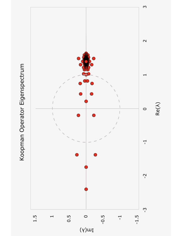
The operator $`\mathcal{K} = e^G`$ has eigenvalue structure $`\lambda_i = e^{-i\omega_i + \gamma_i}`$, $`|\lambda_i| = e^{\gamma_i}`$, where $`\omega_i`$ are eigenvalues of $`H`$ (oscillation frequencies) and $`\gamma_i`$ are eigenvalues of $`\Gamma`$ (growth/decay rates). The Hamiltonian $`H`$ governs unitary evolution ($`|\lambda_i| = 1`$, reversible) when $`\gamma_i = 0`$ for all $`i`$. Language generation instead requires dissipative evolution with $`\gamma_i \neq 0`$: decay modes $`\gamma_i < 0`$ enable information forgetting, growth modes $`\gamma_i > 0`$ enable amplification, and neutral modes $`\gamma_i = 0`$ preserve information. This structure is analogous to Lindblad master equations governing open quantum systems, where the dissipator $`\Gamma`$ describes decoherence, decay, and environmental coupling.
Linear Attention as Context-Dependent Evolution
Language generation requires non-local interactions: the next-token prediction at position $`t`$ must incorporate information from all previous tokens at positions $`0, 1, \ldots, t - 1`$. In physical terms, this is analogous to retarded interactions respecting causal light-cone structure. Position $`t`$ can only “see” its causal past.
The attention mechanism. Attention implements this non-local aggregation through a query-key-value paradigm. At position $`t`$, the hidden state $`\psi_t`$ generates:
\begin{align}
\text{Query:} \quad q_t &= W_Q\psi_t, \\
\text{Keys:} \quad k_s &= W_K\psi_s \quad (s \leq t), \\
\text{Values:} \quad v_s &= W_V\psi_s \quad (s \leq t),
\end{align}where $`W_Q, W_K, W_V \in \mathbb{R}^{d \times d}`$ are learned projection matrices. These are fixed global parameters determined during training and remain constant throughout generation.
Linear Attention. To preserve exact solvability while retaining context aggregation, we employ Linear Attention with bilinear feature map kernels :
\begin{equation}
\text{LinearAttention}(Q, K, V) = \phi(Q)\left(\phi(K)^\top V\right),
\end{equation}where $`\phi : \mathbb{R}^d \to \mathbb{R}^d`$ is a feature map applied element-wise. At position $`t`$, this aggregates information as:
\begin{equation}
\psi_{\text{target},t} = \sum_{s=0}^{t} w_{ts} \cdot v_s, \quad w_{ts} = \phi(q_t)^\top\phi(k_s),
\end{equation}with $`q_t = W_Q\psi_t`$, $`k_s = W_K\psi_s`$, $`v_s = W_V\psi_s`$.
Affine feature map. We employ affine feature maps $`\phi(x) = x + c`$ where $`c \in \mathbb{R}^d`$ is a learned constant vector to enhance expressiveness while maintaining linearity.
Causal structure. Linear Attention respects causality through the summation bound $`s \leq t`$. Position $`t`$ aggregates information only from its causal past $`\{0, 1, \ldots, t\}`$, implementing the light-cone constraint of (1+1)D field theory.
Layered architecture. The model comprises $`L`$ layers, each with propagator $`U^{(\ell)} = \mathcal{K}^{(\ell)}`$, composing as:
\begin{equation}
\psi^{(L)} = \prod_{\ell=1}^{L} U^{(\ell)} \psi^{(0)}.
\end{equation}The Koopman operators $`\mathcal{K}^{(\ell)}`$ are position-dependent, encoding attention through their time-varying structure.
Guided Feynman Path Integrals
Standard Hamiltonian path integrals employ Gaussian measures, restricting eigenvalues to the unit circle $`|\lambda| = 1`$. We generalize to Fresnel integrals: complex Gaussian measures accommodating dissipative spectra $`|\lambda| \neq 1`$. We extend to affine dynamics $`d\psi/dt = G\psi + \beta`$ with bias $`\beta \in \mathbb{C}^d`$. The closed-form solution is:
\begin{equation}
\psi(T) = e^{GT}\psi_0 + G^{-1}(e^{GT} - I)\beta.
\label{eq:affine_solution}
\end{equation}Attention modifies standard Feynman path integration by introducing a context-dependent target state $`\psi_{\text{target},t}`$ aggregating past hidden states. The path integral is then guided via Gaussian weight:
\begin{equation}
W[\psi] = \exp\left(-\frac{1}{2\sigma^2}\|\psi(T) - \psi_{\text{target},t}\|^2\right),
\end{equation}where $`\sigma^2`$ controls guidance strength. This yields the propagator $`K(\psi_1, \psi_0) = \mathcal{N}(\psi_1; \nu, \Lambda)`$ with covariance:
\begin{equation}
\Lambda^{-1} = \Sigma_T^{-1} + \frac{1}{\sigma^2}W_k^\top W_k,
\end{equation}and mean:
\begin{equation}
\nu = \Lambda\left[\Sigma_T^{-1}\left(e^{GT}\psi_0 + G^{-1}(e^{GT} - I)\beta\right) + \frac{1}{\sigma^2}W_k^\top W_q\psi_0\right].
\end{equation}Detailed derivation provided in Supplementary Material Sec. I.
Piecewise constant structure. Within each token interval, parameters $`G_t`$, $`\beta_t`$, $`\Sigma_{T,t}`$ remain constant, enabling exact path integral evaluation. At token boundaries $`t \to t+1`$, parameters undergo discrete jumps: the updated generator $`G_{t+1}`$ incorporates attention to the newly added token, rolling up contributions from all previous positions $`\{0, 1, \ldots, t\}`$ into the propagator structure. This sequential aggregation (smooth intra-token evolution punctuated by inter-token context expansion) is essential for exact solvability while maintaining causal information flow.
Multi-Token Propagation
Multi-token generation chains position-specific propagators with accumulated bias:
\begin{equation}
\psi_N = U_N U_{N-1} \cdots U_1 \psi_0 + \sum_{k=1}^{N} \left(\prod_{j=k+1}^{N} U_j\right) b_k,
\label{eq:multitoken}
\end{equation}where $`U_t = e^{G_t T}`$ is the propagator at position $`t`$ and $`b_k`$ is the bias vector at position $`k`$. This has recursive computational form $`\psi_{k+1} = U_{k+1}\psi_k + b_{k+1}`$. The bias accumulation represents information injection at each position, essential for next-token generation as purely linear dynamics $`\psi_N = U_{\text{total}}\psi_0`$ cannot capture new information not present in $`\psi_0`$.
Progressive Training
We develop a progressive training framework that gradually lifts highly nonlinear transformer architectures to exactly solvable linear dynamics. The strategy: begin with simple spectral methods, progressively add complexity while maintaining mathematical structure, culminating in closed-form propagators.
Stage I: Spectral Foundation with Causal Structure
We initialize with causal Fourier architecture (FNetAR) that respects autoregressive structure:
\begin{equation}
\text{FNetAR}(X)_i = \text{Re}(\mathcal{F}_1(X_{1:i}))_i,
\end{equation}where $`X_{1:i}`$ denotes the causal slice containing only positions 1 through $`i`$, and $`\mathcal{F}_1`$ denotes the 1D discrete Fourier transform. At each position $`i`$, we compute the Fourier transform over the available history, extract component $`i`$, and take the real part. This implements retarded interactions: information propagates forward only.
Each layer implements:
\begin{equation}
x^{(\ell)} = x^{(\ell-1)} + \text{FNetAR}(x^{(\ell-1)}) + \text{MLP}(x^{(\ell-1)}),
\end{equation}where FNetAR includes layer normalization (LayerNorm) (standardizing to zero mean and unit variance with learned affine rescaling) prior to the causal Fourier transform. The MLP is a nonlinear feed-forward map $`\text{MLP}(h) = W_2 \, \phi(W_1 h + b_1) + b_2`$ with $`W_1 \in \mathbb{R}^{4d \times d}`$, $`W_2 \in \mathbb{R}^{d \times 4d}`$, and activation $`\phi(x) = \frac{x}{2}[1 + \text{erf}(x/\sqrt{2})]`$ (Gaussian error linear unit, GELU), providing inter-mode coupling. Training on TinyStories to convergence provides structured initialization for subsequent stages.
Stage II: Koopman Operator Learning
We initialize embedding layers and output projections from Stage I, while the Koopman matrices $`K^{(\ell)} \in \mathbb{C}^{d \times d}`$ are randomly initialized. Training proceeds in two phases. (1) Frozen transfer: Transfer embeddings $`(W_{\text{tok}}, W_{\text{pos}})`$, final layer norm, and output projection from Stage I. Freeze these parameters and train only the Koopman matrices $`\{K^{(\ell)}\}`$ for an initial period. (2) Joint fine-tuning: Unfreeze all parameters and train jointly until convergence.
Each layer applies:
\begin{align}
h^{(\ell)} &= \text{LayerNorm}(x^{(\ell-1)}), \\
k^{(\ell)} &= K^{(\ell)} h^{(\ell)}, \\
x^{(\ell)} &= x^{(\ell-1)} + k^{(\ell)} + \text{MLP}(h^{(\ell)}),
\end{align}where normalization provides numerical stability and the MLP enables inter-mode coupling during training. Spectral analysis after training reveals eigendecomposition $`\mathcal{K}^{(\ell)} = V^{(\ell)}\Lambda^{(\ell)}(V^{(\ell)})^{-1}`$ with absolute values of the eigenvalues typically ranging from 0.1 to 2.0, confirming the non-conservative nature. However, the Stage II Koopman operator alone only achieves a validation loss of $`\approx 3.5`$, slightly better than the Stage I loss of $`\approx 3.7`$, but significantly higher than the baseline transformer loss of $`\approx 2.7`$.
Stage III: Koopman + LinearAttention Hybrid
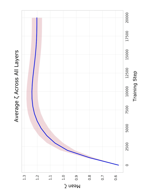
We initialize Koopman operators $`\{K^{(\ell)}\}`$, embeddings $`(W_{\text{tok}}, W_{\text{pos}})`$, and output projection from Stage II. The LinearAttention parameters $`(W_Q, W_K, W_V)^{(\ell)}`$, affine feature map constants $`c^{(\ell)} \in \mathbb{R}^d`$, and layer-wise mixing coefficients $`\zeta^{(\ell)}`$ are randomly initialized. The hybrid architecture:
\begin{equation}
x^{(\ell)} = x^{(\ell-1)} + K^{(\ell)}(x^{(\ell-1)}) + \zeta^{(\ell)} \cdot \text{LinearAttention}^{(\ell)}(x^{(\ell-1)}),
\end{equation}where $`K^{(\ell)}`$ includes LayerNorm and LinearAttention implements causal context aggregation via Eq. (8) with affine feature map $`\phi(x) = x + c`$. Full linearity is achieved when LayerNorm is replaced with simple linear scaling (element-wise multiplication by learned weights), enabling closed-form propagators. The mixing coefficients $`\zeta^{(\ell)} \in \mathbb{R}`$ are learnable parameters controlling the relative contribution of local Koopman evolution versus non-local attention. Layer-wise strengths evolve naturally during training, typically ranging from 0.6 to 1.3, demonstrating the strong modulation that the Koopman operator receives from LinearAttention (Fig.1). Training details in Supplementary Material Sec. II.
 style="width:39.0%" />
 style="width:37.0%" />
Stage IV: Hamiltonian Constraint
To test dissipative necessity, we enforce Hamiltonian structure:
\begin{equation}
H = i(W - W^\top), \quad U = \exp(-iH).
\end{equation}This guarantees $`U^\dagger U = I`$ (unitarity), forcing $`|\lambda_i| = 1`$ for all eigenvalues. This limits the degrees of freedom for the Koopman operator system, though we keep the parameter count unchanged during training.
Stage IV exhibits significant performance degradation: validation loss increases from 2.08 (Stage III) to 3.76. Generated text quality deteriorates markedly, exhibiting repetitive word patterns, grammatical errors, and minimal semantic content (Table II).
We systematically ruled out capacity and architectural limitations as the cause. Moderately increasing embedding dimension or increasing depth produced no improvement in validation loss. We further tested whether linearity constraints were responsible by comparing fully linear architectures (affine feature maps, linear FFN, linear scaling normalization) against fully nonlinear architectures (standard MLP with GELU activation, LayerNorm with learned parameters). Under Hamiltonian constraint $`|\lambda_i| = 1`$, both configurations exhibited similar degradation, demonstrating that the performance loss stems not from architectural choices but from the fundamental incompatibility between unitary evolution and language generation.
Experimental Validation
Table 1 presents validation results across all stages.
| Stage | Total Parameters | Val Loss |
|---|---|---|
| Baseline Transformer | 36.3M | 2.73 |
| I: FNetAR with MLP | 42.5M | 3.68 |
| II: Koopman Operator | 36.0M | 3.54 |
| III: Koopman with Atten | 29.4M | 2.08 |
| IV: Hamiltonian with Atten | 29.4M | 3.76 |
Stage III achieves validation loss of 2.08, and when constrains applied loss raises to 3.76, confirming language requires controlled dissipation, not conservation laws.
| Model | Generated Text |
|---|---|
| Baseline Transformer | “there was a big house in a big house with many toys. One day, a little girl named Lily. She was very happy because she was very curious about everything…” |
| FNetAR with MLP | “both laughed and down and fluffy. Once upon a dull. She said, I will help, you how to play with joy…” |
| Koopman Operator | “there was a little girl called out, and said, call for a time there was sad and always remembered what do. She is a little…” |
| Koopman with Atten | “there was a boy named Timmy. Timmy loved to play with his cars and trucks. One day, Timmy’s mom told him…” |
| Hamiltonian with Atten | “were Everyone been very pair Joezhello saableuckSince because from money wide once ledent who vanilla started Fin withThom the counter insects…” |
Generated text quality by stage. Stage III achieves coherent text comparable to transformer.
Conclusion
We have proven that closed-form quantum path integral solutions can generate coherent language, establishing the Quantum Sequential Field (QSF) as the mathematical foundation for autoregressive sequence modeling. The QSF exhibits (1+1)D dissipative quantum field theory structure: embedding as spatial coordinate, token sequence as temporal evolution, with position-dependent propagators exhibiting sequential parameter updates at token boundaries.
Stage III generates coherent narratives with proper temporal flow. Stage IV’s degraded output (repetitive, minimal semantic content) empirically validates that Hamiltonian constraints fundamentally mismatch language requirements. Table 2 compares generated text using the prompt “Once upon a time” with extended examples provided in Supplementary Material Sec. III.
The four-stage progressive training lifts highly nonlinear transformers to exactly solvable QSF dynamics, reducing perplexity from 15.53 (loss 2.73) for the baseline transformer to 8.00 (loss 2.08) on TinyStories. The mathematical structure reveals language as a dissipative open quantum system where next-token generation admits closed-form solution via generalized Feynman path integrals, and sentence-level generation emerges from chaining position-dependent propagators with accumulated bias injection.
The QSF framework demonstrates that dissipative quantum dynamics, not conservative Hamiltonian evolution, provides the mathematical structure for language generation.
The author thanks Peter W. Milonni for valuable discussions on open quantum systems and path integral methods. This research was supported by Quantum Strategics Inc.
99
S. Greydanus, M. Dzamba, and J. Yosinski, Hamiltonian neural networks, Adv. Neural Inf. Process. Syst. 32 (2019).
Ricky T. Q. Chen, Y. Rubanova, J. Bettencourt, and D. K. Duvenaud, Neural ordinary differential equations, Adv. Neural Inf. Process. Syst. 31 (2018).
B. O. Koopman, Hamiltonian systems and transformation in Hilbert space, Proc. Natl. Acad. Sci. U.S.A. 17, 315 (1931).
I. Mezić, Spectral properties of dynamical systems, model reduction and decompositions, Nonlinear Dyn. 41, 309 (2005).
G. Lindblad, On the generators of quantum dynamical semigroups, Commun. Math. Phys. 48, 119 (1976).
J. L. Ba, J. R. Kiros, and G. E. Hinton, Layer normalization, arXiv:1607.06450 (2016).
A. Vaswani et al., Attention is all you need, Adv. Neural Inf. Process. Syst. 30 (2017).
A. Katharopoulos, A. Vyas, N. Pappas, and F. Fleuret, Transformers are RNNs: Fast autoregressive transformers with linear attention, Proc. Int. Conf. Mach. Learn., pp. 5156–5165 (2020).
J. Lee-Thorp, J. Ainslie, I. Eckstein, and S. Ontañón,, FNet: Mixing tokens with Fourier transforms, Proc. Conf. North Am. Chapter Assoc. Comput. Linguist.: Hum. Lang. Technol., pp. 4296–4313 (2022).
R. Eldan and Y. Li, TinyStories: How small can language models be and still speak coherent English? arXiv:2305.07759 (2023).
📊 논문 시각자료 (Figures)