Random Multiplexing

To address this issue, orthogonal time frequency space (OTFS) [7] and affine frequency division multiplexing (AFDM) [8] techniques have been proposed in recent years to constructing sparse or nearly sparse equivalent channel matrices to suppress the ISI. Although considerable progress has been made, the development of low-complexity and highreliability detection algorithms capable of achieving maximum a posteriori (MAP) BER performance for OTFS and AFDM systems remains an open challenge. State-of-the-art lowcomplexity and replica-optimal signal recovery algorithms, such as approximate message passing (AMP) [9], orthogonal AMP (OAMP) [10], vector AMP (VAMP) [11], and memory AMP (MAMP) [12], offer potential solutions for these scenarios. However, their theoretical analyses and coding designs are generally predicated on assumptions of independent and identically distributed (IID) or right-unitarily invariant channel matrices [9]- [15]. In practical applications, channel distributions often deviate from these assumptions, resulting in performance degradation.

In a nutshell, existing multiplexing, signal detection, and coding design techniques are heavily dependent on specific assumptions regarding channel matrix structures, such as cyclic Toeplitz matrices of static multipath channels in OFDM [1] and single-carrier frequency-domain equalization (SC-FDE) [16], doubly selective channels for OTFS [7] and AFDM [8], which substantially restricts their applicability to complex and dynamic real-world wireless channels.

In static multipath channels, the design principle of OFDM [1] and SC-FDE [16] is to avoid ISI by converting the equivalent frequency-domain channels into multiple parallel singleinput single-output (SISO) channels through orthogonalization, thereby enabling signal recovery using minimum meansquare error (MMSE) detection. However, the orthogonality no longer holds in time-varying doubly-selective channels. To address this issue, OTFS multiplexes information symbols over the delay-Doppler domain, enabling the receiver to mitigate ISI by separating signals based on time delay and Doppler shift [7]. Independently, in AFDM, inverse discrete affine Fourier transform (IDAFT) modulates information symbols in the time-frequency domain, effectively separating signals at the path in terms of time delay and Doppler shift [8]. Both AFDM and OTFS result in sparse or nearly sparse equivalent channel matrices, which facilitates the design of low-complexity signal detection and channel estimation algorithms. Nevertheless, OTFS and AFDM can achieve near-full and full diversity, respectively, when utilizing maximum likelihood (ML) detectors, albeit with prohibitively high complexity. However, guaranteeing the full diversity advantage with practical lowcomplexity detection algorithms remains an open challenge. To tackle these challenges, the interleave frequency division multiplexing (IFDM) has been proposed [17] (see also earlier closely related works in [18], [19]). It utilizes an inverse fast Fourier transform (IFFT) cascaded with a random interleaver to construct an equivalent dense and input-isotropic channel matrix. On this basis, IFDM can effectively cope with the doubly selective fading in time-varying multipath channels, ensuring reliable signal transmission. However, in IFDM, the interleaved-IDFT matrix’s deterministic structure precludes channel-adaptive randomization-a necessity for 6G’s dynamic environments.

In wireless communication systems, when channel state information (CSI) is available to the transceiver, power allocation optimization is typically used to minimize symbol (or bit) error probability or maximize the transmission rate. The traditional approach involves decomposing the wireless channel into multiple parallel single-input single-output (SISO) channels using singular value decomposition (SVD), followed by power allocation to each sub-channel to maximize capacity. For Gaussian signaling, Gaussian waterfilling is employed [20,Sec. 10.4], while mercury waterfilling is applied for discrete signaling [21]. Although the SVD-based power allocation scheme is simple in design, it requires independent channel encoders and decoders with different rates to be assigned to each sub-channel, resulting in a highly complex practical system implementation. To address this difficulty, a power allocation solution based on a specific detector design is explored [19], [22]- [24]. In [22], [23], for Gaussian multiple access channels, power allocation is optimized for iterative multiuser detectors via linear programming to improve BER performance. For MIMO channels, in [24], a power allocation optimization scheme is proposed based on iterative linear minimum mean-square error (LMMSE) detection and discrete signaling, aiming to achieve the maximum achievable rate of the MIMO system. On this basis, a single code is designed that achieves a significantly higher rate than the multicode design for the SVD-based waterfilling scheme, while maintaining comparable encoding and decoding complexity for both schemes. Additionally, an optimal power allocation scheme is proposed for a belief propagation (BP)-based itera-tive receiver, an early version of the OAMP/VAMP1 receiver [10], [11], in energy-spreading-transform (EST)-based MIMO systems [19]. The aim is to achieve the target BER while minimizing transmit power. Meanwhile, it is noted that EST can be considered a special case of the random multiplexing investigated in this paper. However, SVD-based optimal power allocation in [20], [21] does not guarantee optimal MAP BER (see Fig. 13), only capacity optimal, but relies on multiple AWGN capacity-achieving channel codes with different rates. Moreover, detector-based optimal power allocation in [19], [24] requires high-complexity LMMSE detection, which is challenging to implement in large-scale systems due to its prohibitive complexity.

AMP-type algorithms have been extensively studied for signal recovery in linear systems, owing to their low complexity and high efficiency in high-dimensional settings. In particular, the low-complexity AMP algorithm has been shown to be Bayes-optimal via scalar state evolution (SE) analysis [25], [26], but it easily diverges when applied to non-independent and identically distributed (IID) measurement matrices. To overcome this limitation, a convolutional AMP was proposed for general rotationally invariant matrices [27], but it suffers from slow convergence and instability under high condition numbers. Alternatively, a long-memory AMP has been shown to be effective for right-unitarily invariant matrices [28]. Another line of work is OAMP/VAMP, whose Bayes optimality under right-unitarily invariant matrices has been established via replica methods [29], [30], and later proven under specific spectral constraints [31], [32]. However, their reliance on high-complexity LMMSE detectors limits scalability. To address this, MAMP replaces LMMSE with a low-complexity memory matched filter (MF), retaining Bayes optimality. Independently, a warm-start conjugate gradient VAMP (WS-CG-VAMP) was proposed in [33], leveraging conjugate gradient methods for similar complexity reduction. The convergence of OAMP/VAMP and MAMP with optimized damping has been established in [12], [34], [35]. Moreover, AMP-type algorithms have been shown to exhibit universal behavior across a wide range of random matrices, including IID, rightunitarily invariant, sign/permutation-invariant, certain Wignerresolvent, and delocalized orthogonal ensembles [36], [37].

More recently, AMP-type algorithms have been applied to signal recovery in multiplexing systems. For instance, a crossdomain (CD) OAMP/VAMP, inspired by the turbo compressed sensing algorithm [38], was proposed for OTFS [39]. Additionally, a delay-Doppler OAMP/VAMP (DD-OAMP/VAMP) was introduced in [40]. However, these methods struggle to exploit the sparsity of channel matrices in the time or delay-Doppler domain because of the matrix multiplication and inversion required in LMMSE detection. To this end, a lowcomplexity DD-MAMP detector has been proposed in [41], incorporating a memory MF to leverage the channel sparsity in delay-Doppler domain. Nevertheless, it neglects the greater Fig. 1: A comparison of the equivalent channel matrices H eqv output×input = Ξ H HΞ of OFDM [1] (Ξ = F H ) in static multipath channels, and OTFS (Ξ = F H ⊗ I) [7], AFDM (Ξ = Λ H c 1 F H N Λ H c 2 ) [8] and the random multiplexing (RM) in Definition 3 in time-varying doubly-selective channels, where H denotes the time-domain channels, Ξ the multiplexing matrix, and Λc i ≜ diag(e -j2πc i n 2

, n = 0, • • •, N -1), i = 1, 2.

sparsity inherent in time-domain channels, leaving a promising avenue unexplored. Besides, the Bayesian optimality of widely used AMP-type algorithms [9]- [12], [25]- [35], [42] relies on specific assumptions on the channel matrices, such as IID and right-unitarily invariant matrices. However, in real-world wireless applications, the channel matrices, including the equivalent channel matrices of common multiplexing schemes such as SC-FDE, OFDM, OTFS, and AFDM, generally do not meet these assumptions required for AMP-type algorithms to achieve optimal performance. Consequently, AMP-type detectors suffer from significant performance degradation, as shown in Fig. 11 and Fig. 12.

Channel coding design is crucial for ensuring reliable communication and approaching the channel capacity in wireless systems. Most modern coding designs are aimed at classical binary erasure channels and binary-input additive white Gaussian noise (AWGN) channels [43], such as Turbo codes [44], low-density parity-check (LDPC) codes [45], spatially coupled LDPC codes [46], Polar codes [47], sparse regression codes [48]- [50]. It should be noted that all of these welldesigned channel codes focus on single-input-single-output (SISO) channels but are suboptimal in linear systems [13]- [15].

To address this challenge, existing literature explored the channel coding optimization for joint AMP-type detection and decoding in linear systems [13]- [15]. In [13], the potential constrained capacity optimality of the AMP receiver for coded linear systems with arbitrary input and IID channel matrices is proven [25], [26], under the assumption that the AMP receiver’s SE is correct and has a unique fixed point. The potential capacity optimality of OAMP/VAMP for rightunitarily invariant matrices and the corresponding optimal coding principle are shown in [14]. To address OAMP/VAMP’s high complexity, the replica capacity-optimal MAMP receiver and its coding principle are established in [15]. Note that when practical wireless channels do not satisfy the IID or rightunitarily invariant conditions, the conclusions of the above studies no longer hold, presenting an ongoing challenge.

To address the aforementioned challenges, we study a random multiplexing framework that unifies and extends the principles of IFDM [17] and EST [18], [19]. This random multiplexing framework employs a random matrix for multiplexing, allowing it to be applied to arbitrary norm-bounded and spectrally convergent channel matrices while ensuring that the equivalent matrices belong to the universality class U [36]. Unlike conventional constellation modulation that focuses on mapping symbol-level information bits to complex constellation points, the random multiplexing studied in this paper focuses on the mapping of high-dimensional complex symbol vectors. Furthermore, random multiplexing can be regarded as a general terminology for existing precoding techniques that reshape the equivalent channel distribution to satisfy the universality class condition, even in practical wireless scenarios. Therefore, random multiplexing preserves the performance limits of linear systems, including the replica MAP BER and constrained channel capacity. As shown in Fig. 1, the equivalent channel matrices of random multiplexing is more densely stable compared to existing OFDM [1], OTFS [7], and AFDM [8], making it easier to ensure reliable signal transmission. To avoid the high complexity of signal detection on equivalent dense matrices, a cross-domain MAMP detection has been considered, which leverages both the sparsity of the time-domain channels and the input isotropy of the equivalent channel matrices. Meanwhile, when CSI is available at the transceiver, power allocation optimization strategies are proposed for random multiplexing systems with arbitrary norm-bounded and spectrally convergent channel matrices, as well as arbitrary discrete signaling, aiming to achieve the replica MAP BER and maximize the constrained capacity, respectively. On this basis, the optimal coding principle and replica capacity optimality of random multiplexing systems are investigated. The main contributions of this paper are summarized as follows:

1. This paper studies a random multiplexing technique that performs a unitary random transformation on the discrete signal vector prior to transmission. The transformation operates independently of both the signal vector and the channel matrix, in contrast to conventional multiplexing schemes that inherently couple the multiplexing matrix with the channel characteristics. This decoupling in random multiplexing simplifies system design and greatly enhances flexibility. Unlike conventional multiplexing schemes that rely on channel sparsification to enable lowcomplexity detection, random multiplexing establishes an equivalent fully dense and input-isotropic channel matrix. This ensures that every signal symbol homogeneously undergoes sufficient statistical channel fading, thereby enhancing overall system performance. Moreover, random multiplexing preserves both the replica MAP BER and the replica constrained capacity of linear systems. The random multiplexing framework includes two key types of random matrices: (i) Haar distributed matrices, and (ii) permutation-invariant matrices, ensuring both the theoretical validity and asymptotic optimality (achieving replica MAP-BER performance) for AMP detection. 2) Based on the state evolution analysis for linear systems, we demonstrate that the power allocation to minimize the replica MAP BER is a bilevel problem (with a concave maximization inner problem), and the power allocation to maximize the replica constrained capacity is a concave maximization problem. Efficient algorithms for solving the optimal power allocations are provided. Compared with conventional Gaussian/mercury waterfilling [20], [21], the proposed scheme achieves a lower MAP BER. In contrast to the BER-minimizing power allocation based on high-complexity iterative LMMSE detector [19], [24], this paper develops power allocation for low-complexity CD-MAMP receivers. Furthermore, we extend our analysis beyond BER minimization to investigate the replica constrained capacity-optimal power allocation.

2. The versatility of random multiplexing in various wireless applications is explored, including its low-complexity random transform, higher spectral efficiency, adaptability to other multiplexing schemes, and support for compressed and spread random multiplexing. 4) Numerical results show that in correlated time-varying multipath MIMO channels, random multiplexing can achieve BER and block-error rate (BLER) performance gains of up to 2 ∼ 10 dB compared to existing schemes (e.g., OFDM/OTFS/AFDM with well-designed SISO codes), under both uniform and optimized power allocation, as well as optimal coding. Part of the results in this paper has been published in [51]. In this paper, we present additional key properties of random multiplexing, detailed proofs, a discussion of potential applications, the design of optimal codes, achievable rate analysis, and further numerical results.

F. Related Works 1) Comparison with Existing Multiplexing Schemes: Existing OFDM [1], SC-FDE [16], OTFS [7], and AFDM [8] rely on constructing diagonalized or sparse equivalent channel matrices for static or time-varying multipath channels to mitigate ISI at the receiver, thereby facilitating signal recovery. However, due to the non-orthogonal structure of the equivalent channel matrices, state-of-the-art (SOTA) lowcomplexity signal detection methods suffer from significant performance degradation (see Fig. 12). In contrast, EST [18], [19] and IFDM [17] enhance signal detection performance by constructing an equivalent input-isotropic channel matrix through interleaved FFT/IFFT, allowing the signal to undergo sufficient statistical channel fading. This paper explores random multiplexing based on a general random transform, which generalizes both IFDM and EST. Additionally, the theoretical optimality of random multiplexing-namely, replica MAP-BER and replica constrained capacity-are provided. Moreover, random multiplexing offers a generalized framework that decouples the multiplexing matrix from the channel matrix, going beyond the conventional channel-coupled OFDM [1], OTFS [7], AFDM [8], and IFDM [17].

2. Connection to the Universality Class U in [36]: The universal behavior of AMP-type algorithms is established in [36] for a broad class of universality class U , including linear transformations of IID matrices, right-unitarily invariant matrices, permutation-invariant matrices, among others. A critical limitation, however, arises for permutation-invariant matrices: The analysis in [36] requires channel matrices A to satisfy a restrictive structural condition-specifically, their singular value decompositions must obey A = U A Σ A V H A with V A = I (i.e., the right singular vectors form the identity matrix). In this paper, we overcome this limitation by extending the applicability of permutation-invariant matrices to more general off-diagonal-sum constrained channel matrices, a broader class that subsumes the earlier restrictive case. Furthermore, we conjecture that these results may generalize to arbitrary norm-bounded and spectrally convergent channel matrices, suggesting a potentially universal framework beyond currently verifiable cases.

3. Comparison with Existing Detection Algorithms: Stateof-the-art AMP-type signal recovery algorithms (e.g., OAMP [10], VAMP [11], and MAMP [12]) have been studied and applied to existing multiplexing systems, including CD/DD-OAMP/VAMP [39], [40] and DD-MAMP [41]. However, these algorithms require the channel matrix to exhibit a specific right-unitary invariance property. This requirement is typically unmet by practical communication channels, resulting in significant performance degradation (see Fig. 11). Random multiplexing ensures that the equivalent channel matrix consistently satisfies the input isotropy, regardless of the distribution of the original channel. This guarantees the validity of the AMPtype detection algorithms. Specifically, a low-complexity CD-MAMP detector is considered for random multiplexing systems, which is extended from the specific interleaved-IDFT matrix applicable in IFDM [17] and interleaved block-sparse transform (IBST) matrix [52] to the more general unitary random transformation matrices, including but not limited to Haar distributed matrices and permutation-invariant matrices

∼ Unif [0, 2π) , Π is a uniformly random permutation matrix independent of D, and U is a delocalized deterministic unitary matrix (e.g., DFT, Hadamard-Walsh, DCT) satisfying ∥U ∥ max ≲ N -1/2+ϵ for any ϵ > 0. By exploiting the isotropy of the transformdomain channel, CD-MAMP preserves the desirable properties, including rigorous state evolution analysis, replica Bayes optimality, and low-complexity implementation. Furthermore, CD-MAMP introduces a cross-domain processing mechanism that leverages the time-domain channel sparsity and fast transformation, lowering the complexity to O(KN + N log N ), where K is the the number of non-zero elements per row in time-domain channel matrix H, without sacrificing performance. These make CD-MAMP a competitive solution for signal detection in random multiplexing systems, delivering both replica Bayes-optimal performance and computational efficiency.

4. Distinct from Existing Power Allocation Methods: The conventional power allocation methods use SVD channel decomposition followed by water filling of the power [20], [21], but they overlook the need for multiple capacity-achieving codes to achieve the channel capacity, which is practically prohibitive. Meanwhile, the state-of-the-art detector-based power allocation methods in [19], [24] are constrained by the highcomplexity iterative receivers involving LMMSE estimation and limited to the replica MAP BER minimization. To this end, leveraging the advantages of random multiplexing, this paper proposes optimal power allocation strategies for lowcomplexity CD-MAMP detectors, aiming to minimize the replica MAP BER and maximize the replica constrained capacity, respectively.

5. Distinct from Well-Designed Channel Codes: Conventional channel coding designs focus on overcoming the effects of channel noise to achieve the SISO AWGN channel capacity [43], but they remain strictly suboptimal in linear systems [13]- [15]. While AMP-type detectors achieve capacity optimality under right-unitary invariant matrices [13]- [15], this assumption rarely holds in practical wireless systems. In contrast, random multiplexing ensures the input isotropy of the equivalent channel matrices, integrating the low-complexity CD-MAMP detection to effectively address this gap by enabling accurate performance characterization via state evolution, while maintaining replica Bayesian optimality. This establishes the optimal coding principle and replica-capacity optimality to be applied to linear systems with arbitrary normbounded and spectrally convergent channel matrices, as well as arbitrary signaling schemes.

Lowercase letters denote scalars and boldface lowercase letters denote vectors. [•] T and [•] H denote transpose and conjugate transpose operations, respectively. I denotes the identity matrix of appropriate size. I(x, y) denotes mutual information between x and y. |S| is the cardinality of a set S. tr(A) and det(A) are the trace and the determinant of A, respectively. ∥a∥ denotes the ℓ 2 -norm of a vector a. E{•} denotes the expectation over all random variables included in the brackets. E{a|b} denotes the conditional expectation of a for given b. mmse{a|b} represents E{|a -E{a|b}| 2 |b}. CN (µ, Σ) represents the circularly-symmetric Gaussian distribution with mean µ and covariance matrix Σ.

[N ] denotes the set {1, • • •, N }. ∥A∥ max ≡ max i,j |A i,j | denotes the max norm, ∥A∥ 2 denotes the spectral norm. f -1 (•) denotes the inverse function of f (•), and 1/f (•) or [f (•)] -1 denotes the multiplicative inverse. We write a N ≲ b N to indicate that

for some constants C > 0 and N 0 > 0.

Definition 1 (Spectrally Convergent Matrix). A matrix A is said to be spectrally convergent if the empirical spectral distribution of A H A converges to a compactly supported probability distribution. Specifically, for any fixed

where µ denotes a compactly supported probability distribution on [0, ∞).

This paper is organized as follows. Section II presents the preliminaries. Section III introduces the random multiplexing and its advantages. In Section IV, we consider CD-MAMP detection for random multiplexing. Section V focuses on optimal power allocation techniques, while Section VI introduces the optimal coding principle for random multiplexing. The extended applications of random multiplexing are explored in Section VII, followed by numerical results in Section VIII.

This section introduces the norm-bounded spectrally convergent linear systems and the mercury/waterfilling scheme.

A. Norm-Bounded and Spectrally Convergent Linear Systems Consider a linear system with power allocation:

where A = HP , H ∈ C M ×N is a channel matrix, P ∈ C N ×N a power allocation matrix subject to tr{P P H } = P sum , y ∈ C M ×1 a vector of observations, x ∈ C N ×1 a vector to be estimated, and n ∈ C M ×1 a noise vector. When P = I, it reduces to the uniform power allocation. Without loss of generality, the average powers of P and x are normalized, i.e., P sum = N and 1 N ∥x∥ 2 a.s. = 1, where a.s.

= denotes almost sure convergence. Let snr = σ -2 represent the transmitsignal-noise ratio (SNR). In addition, we impose the following assumptions on A, x, and n. Assumption 1. We consider a large-scale linear system that M, N → ∞ with a fixed δ = M/N . The measurement matrix A is spectrally convergent (see Definition 1) and has a bounded spectral norm satisfying ∥A∥ 2 ≲ 1. The entries of x are IID distributed, i.e., x i.i.d. ∼ P x . The noise vector is IID Gaussian, i.e., n ∼ CN (0, σ 2 I) for some σ > 0. In addition, x, n and A are mutually independent.

Note that, unlike AMP-type algorithms, which typically rely on specific isotropy assumptions for A (e.g., IID or unitary invariance), Assumption 1 significantly relaxes the constraints on the matrix A. Specifically, it allows A to be any norm-bounded and spectrally convergent matrices, thereby encompassing a broad spectrum of practical applications. These include, but are not limited to, inter-symbol interference (ISI) equalization, compressed sensing, multiple-input multiple-output (MIMO), multiple-access channels (MAC), random access, channel estimation, channel coding, etc [53], [54]. This generality makes the framework applicable to a wide range of real-world problems beyond the limitations of traditional AMP-based approaches.

Let R R (•) denote the R-transform with a Hermitian matrix R, as defined in [55]:

where S -1 R (•) is the inverse function of the Stieltjes transform:

The MMSE and BER metrics are widely recognized as important criteria in signal processing and communication. The theoretical MMSE and symbol-wise MAP BER of a linear system in (3) under individually optimal detection can be predicted by the replica method as follows.

Lemma 1 (Replica MMSE and MAP BER). Under Assumptions 1, the MMSE of the linear system in (3) can be predicted by solving the fixed-point equation for v * :

which is derived from the replica method [29], [30]. Correspondingly, the replica MAP BER is

where

with the a posteriori mean

and Q S (ρ) denotes the MAP demodulation BER for √ ρx + z under the signal constellation constraint x ∈ S (See Appendix A for details).

Remark: The replica method is heuristic, based on an unjustified exchange of limits and an unsupported replica symmetry assumption. If the fixed point is unique, it is conjectured that the replica MMSE equals the true MMSE for right unitarily-invariant matrices A. Currently, this conjecture has only proven for IIDG matrices [25], [26] and a specific sub-class of rotationally-invariant matrices [31], [32].

Assumption 2 (Unique Fixed Point). Assume that the fixedpoint equation in (5), derived from the replica method [29], [30] for the linear systems in (3), has a unique solution v * .

Channel capacity is a common metric for performance limit in communication systems. The following lemma, proven in [56], establishes the connection between MMSE and the constrained capacity of a SISO AWGN channel given P x .

Lemma 2 (Scalar I-MMSE [56]). The constrained capacity of a SISO-AWGN channel is

Based on Lemmas 1 and 2, the replica constrained capacity of a linear system in (3) is presented in the following lemma.

Lemma 3 (Replica Constrained Capacity [29], [30], [32]). Under Assumptions 1 and 2, the constrained capacity (per transmit symbol) of the linear system in (3), as predicted by the replica method, is given by:

where R R (•) is the R-transform given in (4) with R = A H A, and C SISO (•) is given in (8).

The existing researches on the optimal transceiver faces the following two challenges, depending on whether CSI is available at the transmitter:

1. CSI Known at Transceivers: Traditional approaches decompose wireless channels into parallel SISO channels via SVD, enabling capacity to be achieved using multiple SISO capacity-achieving codes rather than a single code. This would bring an extremely high-complexity challenge, rendering it impractical in numerous practical communication systems. Furthermore, although mercury/waterfilling can maximize the constrained capacity of the underloaded linear systems [21], it does not guarantee achieving the MAP BER when considering only the BER performance of detection. As a result, optimizing power allocations to minimize the MAP BER and achieve the maximal constrained capacity using a single code remains an open challenge.

2. CSI Known Only at Receiver: For practical large-scale communication systems, acquiring the accurate CSI at the transmitter is difficult and expensive, while the complexity of implementing SVD and water filling incurs significant computational overhead, particularly for low-cost terminal devices. Additionally, when the channel experiences rapid and frequent changes, repeatedly acquiring CSI and performing SVD for each channel change becomes impractical. In practice, it is commonly assumed that CSI is unknown at the transmitter, in which conventional techniques such as SVD and waterfilling cannot be employed. In such cases, the optimal strategy is to adopt an identical uniform power distribution, i.e., x i ∼ P x and E{|x i | 2 } = 1 for i ∈ [N ]. Nevertheless, the design of multiplexing, detection, encoding, and decoding algorithms with practical complexity that approach the replica MAP BER or replica constrained capacity of the linear system in (3) remains an open problem. ∼ Ps, and Ξ denotes the RT matrix that is independent of the signal vector s, the measurement matrix A, and the channel noise n.

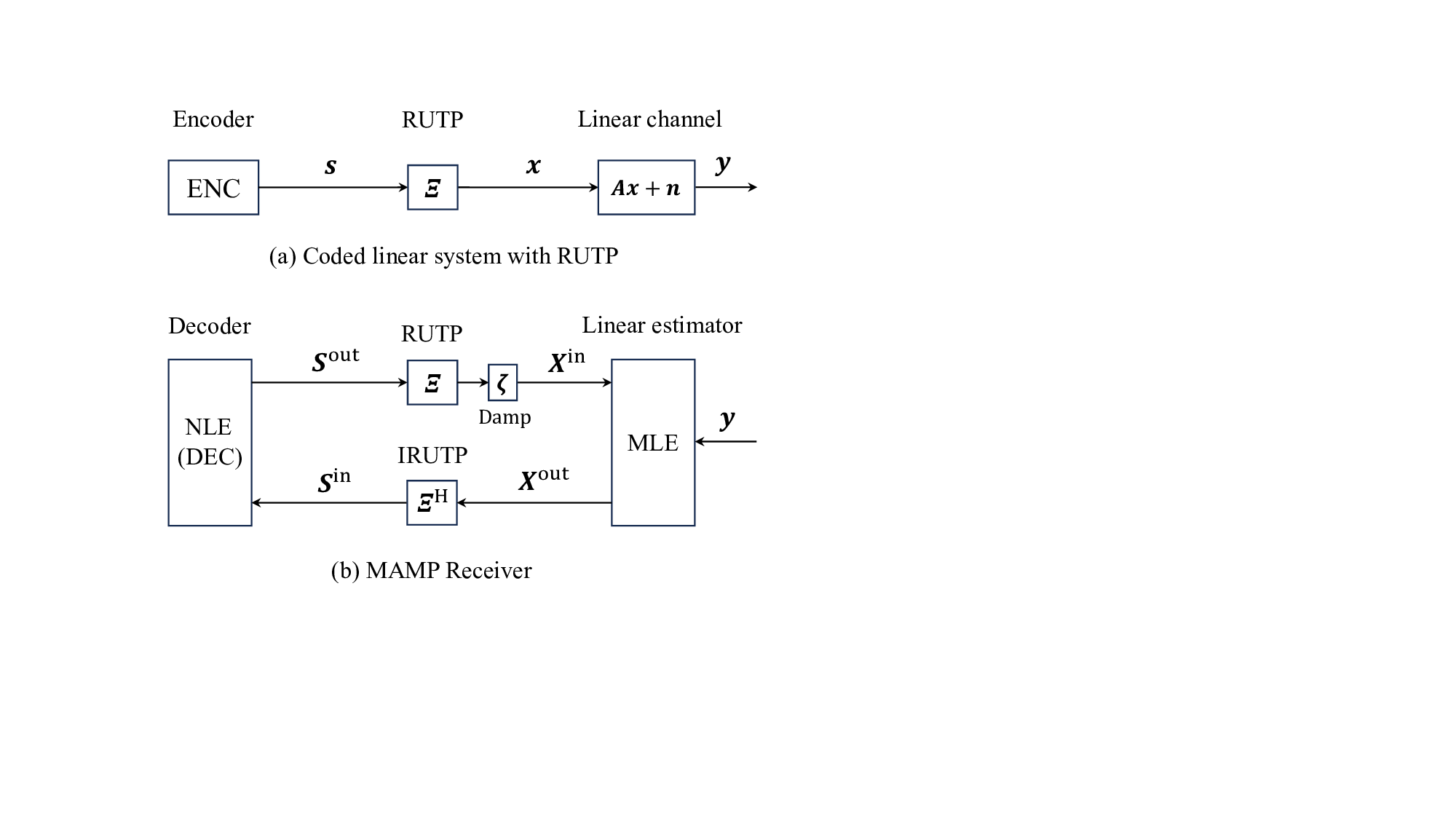
In this section, we introduce random multiplexing and its intrinsic advantages as a practical solution for linear systems.

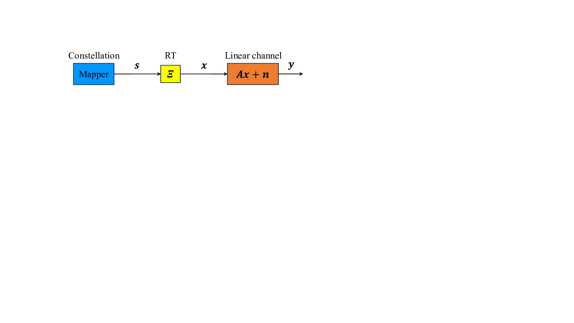
The signal vector s ∈ C N ×1 is modulated by the transform matrix Ξ ∈ C N ×N , i.e.,

where entries of s are IID distributed, i.e., s i.i.d.

∼ P s . As illustrated in Fig. 2, a linear multiplexing system with power allocation can be described by:

As stated in Assumption 1, we assume throughout this paper that A is spectrally convergent and has a bounded spectral norm ∥A∥ 2 ≲ 1. This means that the empirical spectral distribution of A H A converges to a compactly supported distribution, and the largest singular value of A is finite.

Definition 2 (Universal Multiplexing). We refer to Ξs as universal multiplexing of the signal s, if the equivalent channel matrix AΞ lies in the universality class U [36], defined as:

Remark: The universality class U , introduced in [36], plays a pivotal role by ensuring that the dynamics of AMPtype algorithms can be accurately tracked via state evolution. While the original definition of U in [36] is formulated over the real field, we extend it to the complex field in Definition 2. This extension involves replacing real-field concepts with their natural complex counterparts: (i) transposes are replaced with Hermitian transposes, and orthogonal matrices with unitary ones; (ii) the uniformly random sign matrix S (i.e., a diagonal matrix with IID entries from Unif{±1}) is generalized to the uniformly random phase diagonal matrix D. It has been shown in [36] that, over the real field, U ensures that the error vectors in OAMP/VAMP are asymptotically IID Gaussian and thus ensures the accuracy of SE. In this work, we assume that this property also holds in the complex setting.

Lemma 4 (IID Matrices [36]). Suppose that A is spectrally convergent and has a bounded spectral norm ∥A∥ 2 ≲ 1. Then, AΞ IID ∈ U , where the entries of Ξ IID are independently drawn from a circularly symmetric distribution with mean zero and variance 1/N .

The multiplexing matrices Ξ in Definition 2 are broadly defined, covering a wide variety of matrices. In current multiplexing systems, unitary matrices are commonly used as they preserve the channel capacity. For greater flexibility, we further require that Ξ be independent of the channel and signal. These considerations lead us to random multiplexing as defined below.

Definition 3 (Random Multiplexing). We refer to Ξs as random multiplexing of the signal s if:

1. Ξ is a unitary random matrix, satisfying Ξ H Ξ = I, and is independent of {A, s, n}.

2. The equivalent channel matrix AΞ belongs to the universality class U , i.e., AΞ ∈ U .

Based on Definition 3, we refer to Ξ as the random transform (RT) matrix and Ξs as the RT of s. Accordingly, Ξ H and Ξ H s are the inverse random transform (IRT) matrix and the IRT, respectively. Subsequently, we introduce several well-defined classes of the RT matrices Ξ.

Theorem 1 (Permutation-Invariant Matrices). Suppose that A is spectrally convergent, has a bounded spectral norm ∥A∥ 2 ≲ 1, and satisfies the off-diagonal-sum condition:

Then, AΞ PI ∈ U , where

for any ϵ > 0.

Proof: See Appendix B. In the real case, Theorem 1 directly reduces to the formulation corresponding to the original definition of U over the real field in [36]. The result of [36,Lemma 3] is a special case of Theorem 1, where the right singular vectors of A form the identity matrix. For ease of reference, we restated it as the following corollary.

A be the singular value decomposition of A, where V A = I (i.e., the right singular vectors form the identity matrix). Suppose that A is spectrally convergent and satisfies ∥Σ A ∥ 2 ≲ 1. Then, AΞ PI ∈ U .

For Haar-distributed matrices, a subclass of the permutationinvariant matrices, the off-diagonal-sum condition on A in ( 13) is not necessary, yielding the following lemma.

Lemma 5 (Haar-Distributed Matrices [36]). Suppose that A is spectrally convergent and has a bounded spectral norm ∥A∥ 2 ≲ 1. Then, AΞ Haar ∈ U , where the random transform matrix Ξ Haar is Haar distributed, i.e., Ξ Haar ∼ Unif(U(N )), where U(N ) denotes the unitary group.

The Haar measure is distributionally invariant to left or right multiplication by any independent unitary matrices. Hence,

A Ξ Haar is Haar distributed. Furthermore, Ξ has the same distribution as Π ΞD for any independent permutation Π and diagonal phase matrix D. In addition, for any ϵ > 0, ∥ Ξ∥ max ≲ N -1/2+ϵ with probability 1 [57]. Therefore, we apply Corollary 1 to complete the proof.

In practice, we typically set D = I and choose U to be fast transform matrices for the permutation-invariant matrices in Theorem 1. That is, Ξ PT ≡ ΠT , where T denotes fast transform matrices, such as discrete Fourier transform (DFT), Hadamard-Walsh transform (WHT), or discrete cosine transform (DCT), interleaved block-sparse transform [52],

and in orthogonal chirp division multiplexing (OCDM) with c 1 = c 2 = 1 2N . A suitable unitary matrix is selected in accordance with practical application requirements and hardware complexity constraints.

• CSI Known Only at Receiver: Ξ PT represents a special case of that in Theorem 1 with P = I.

• CSI Known at Transceivers: Ξ PT represents a special case of that in Corollary 1 with the optimal form of P (See Theorem 2 in Section V). In addition, Ξ can be also constructed using multi-layer permutation-invariant matrices, expressed as

where each pair {Π l , T l } is randomly selected [18]. However, it remains unproven that the equivalent matrix AΞ ML lies in the universality class U .

1. Decoupling from the Channel Matrix: Conventional multiplexing schemes, such as OFDM, SC-FDE, OTFS, and AFDM, inherently couple the multiplexing matrix with the channel characteristics. In contrast, random multiplexing decouples the multiplexing matrix Ξ from the channel matrix H, i.e., Ξ is independent of H. This decoupling enables random multiplexing to be applied to arbitrary norm-bounded and spectrally convergent channel matrices.

2. Asymptotic Performance Limits: The introduction of RT matrix Ξ in (11) does not change the eigenvalues of A H A. As a result, the random multiplexing in (11) does not lead to any performance or rate loss compared to the original linear systems in (3).

Proposition 1 (Preservation of Replica Limits). Random multiplexing preserves the replica MAP BER and constrained capacity of the original linear systems in (3), including the Gaussian capacity with Gaussian signaling.

Proof: Following Lemmas 1 and 3, both the replica MAP BER and the replica constrained capacity of a linear system are determined by the Stieltjes transform. Define R ≡ (AΞ) H AΞ. We have

where (15c) follows Ξ H Ξ = I. Therefore, the Stieltjes transform of the random multiplexing system is identical to that of the original linear system. Consequently, both the replica MAP BER and the replica constrained capacity remain unchanged in the random multiplexing system.

3. Low-Complexity and Asymptomatically Optimal Receiver: Existing multiplexing matrices Ξ and channel matrices H are typically highly structured, making it challenging for AΞ to exhibit the required input isotropy. This lack of isotropy hampers the development of efficient signal recovery algorithms [39]- [41], with the exception of OFDM in timeinvariant channels, where Ξ H HΞ forms an orthogonal matrix. As shown in Fig. 1, the equivalent channel matrices of OFDM, OTFS, and AFDM exhibit diagonalized and specific sparsification structures in static and time-varying multipath channels, respectively. Specifically, the OTFS multiplexing matrix is [8], a multiplexing matrix Ξ is a sparse Walsh-Hadamard matrix [58], and the ISI channel matrix H is a Toeplitz matrix. As a result, existing AMP-type algorithms in [10]- [12], [27], [28], [33], [59] suffer significant performance losses and are unable to approach the MAP BER or the constrained capacity. Thanks to the random multiplexing in (10), the effective channel matrix AΞ belongs the universality class U , facilitating the utilization of AMP-type receivers, which asymptotically achieve the replica MAP-BER or the replica constrained capacity of the linear systems in (3). Lemma 6 (Replica MAP BER/Capacity Optimality). In random multiplexing systems, we have AΞ ∈ U . Suppose that the Assumptions 1 and 2 hold. Then,

• OAMP/VAMP [10], [11], long-memory AMP [28], PCAinitialized AMP [59], and MAMP [12] can achieve the replica MAP BER in (6), and • OAMP/VAMP and MAMP, utilizing optimal Lipschitzcontinuous decoding (as defined in (52)), can achieve the replica constrained capacity in (9) [14], [15].

In linear systems with random multiplexing, the effective channel matrix AΞ exhibits enhanced stability, enabling each element of s to experience all channel fading effects in A due to the input isotropy of Ξ. Consequently, random multiplexing can potentially attain maximum diversity, thereby improving signal recovery performance. We have not conducted a thorough analysis of the diversity of random multiplexing. However, as demonstrated in Lemma 6, its replica MAP BER optimality suggests that random multiplexing is capable of achieving maximum diversity. Notably, while MAP BER optimality is sufficient to guarantee maximum diversity, the converse does not hold: maximum diversity does not necessarily imply MAP BER optimality.

To visually demonstrate the advantages of multiplexing matrix Ξ, we provide experimental analyses of two-dimensional and high-dimensional random multiplexing linear systems. For simplicity, let M = N and A be invertible. Accordingly, (11) is rewritten as

where

where n ∼ CN (0,

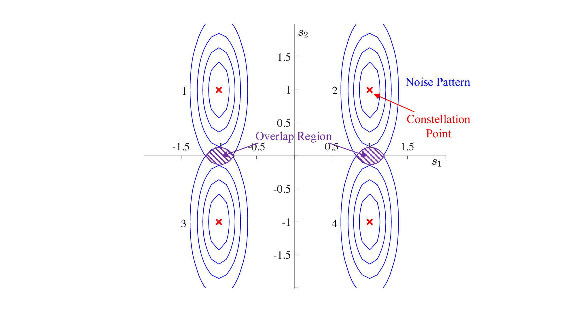
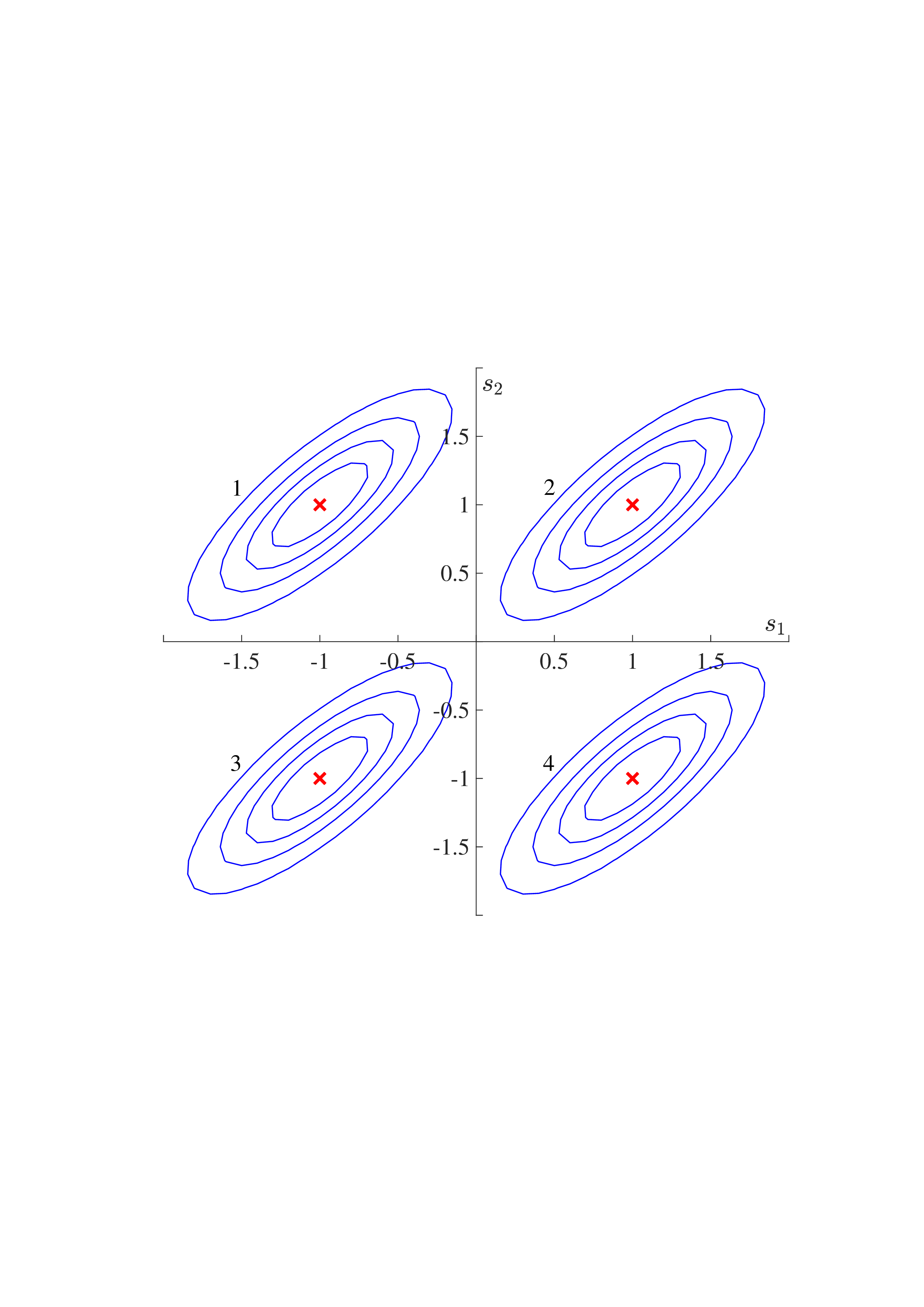
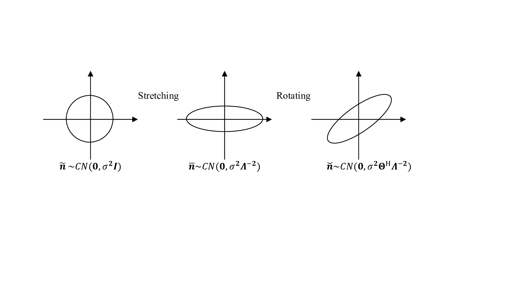
Based on (17), we have the following observations. 1) Example 1: Consider a 2D linear communication system with BPSK signal vector s = [s 1 , s 2 ] T in (17), where σ 2 = 0.1 and Σ A = diag{3/2, 1/2}. We compare the orthogonal and unitary modulations as follows.

• 2D Orthogonal Multiplexing (e.g., OFDM): Assuming Ξ = V A , we obtain an asymmetric noise vector n = (17). That is, s 1 is subject to reduced noise, whereas s 2 experiences increased noise. Consequently, the overall signal recovery performance is affected by the performance of s 1 , leading to deterioration. In Fig. 3(a), we visualize the contour lines of the received signals ȳ affected by asymmetric effective noise n, referred to as noise patterns. In the s 1 direction, the noise patterns are far apart, making them easy to distinguish. Nevertheless, in the s 2 direction, the noise patterns overlap, resulting in poor signal recovery performance.

• 2D Unitary Multiplexing:

] is a 45-degree rotation matrix. As shown in Fig. 3(b), we then get an effective noise vector n = Θ[2/3ñ 1 , 2ñ 2 ] T with symmetric with covariance matrix σ 2 ΘΣ -2

A Θ T = [0.222, 0.177; 0.177, 0.222]. Consequently, the noise pattern of each constellation point is sufficiently distinct from those of the other constellation points, enhancing the overall performance. Fig. 3(c) shows that the BER of the 45-degree rotation multiplexing with ML detection outperforms that of the 2D orthogonal multiplexing.

Challenge: For 2D linear systems, a suitable Ξ can be obtained through meticulous design. However, for highdimensional linear systems, finding a appropriate Ξ is challenging. We investigate the statistical characteristics of a randomly selected Ξ using the experimental setup outlined below for high-dimensional linear systems.

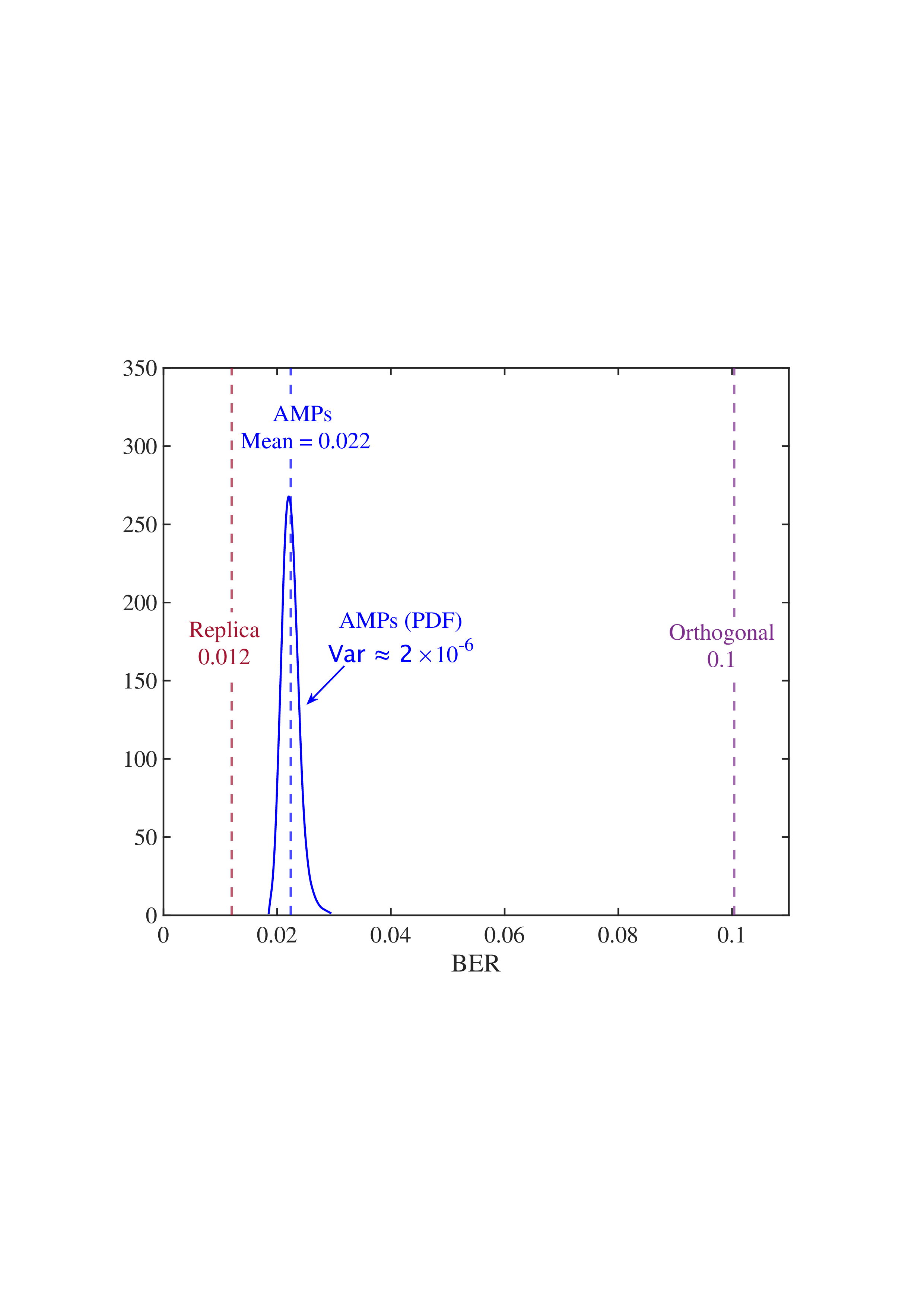
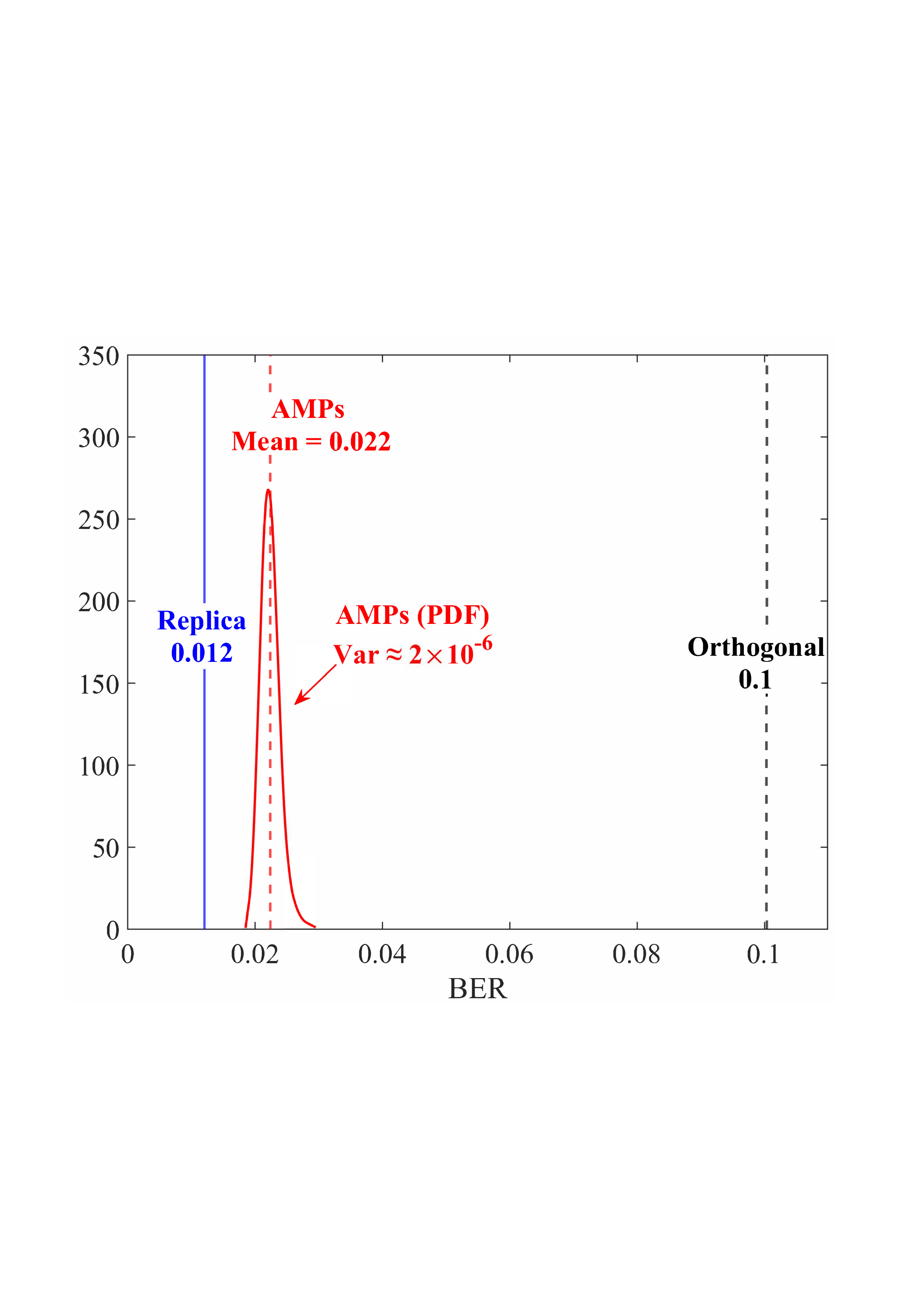
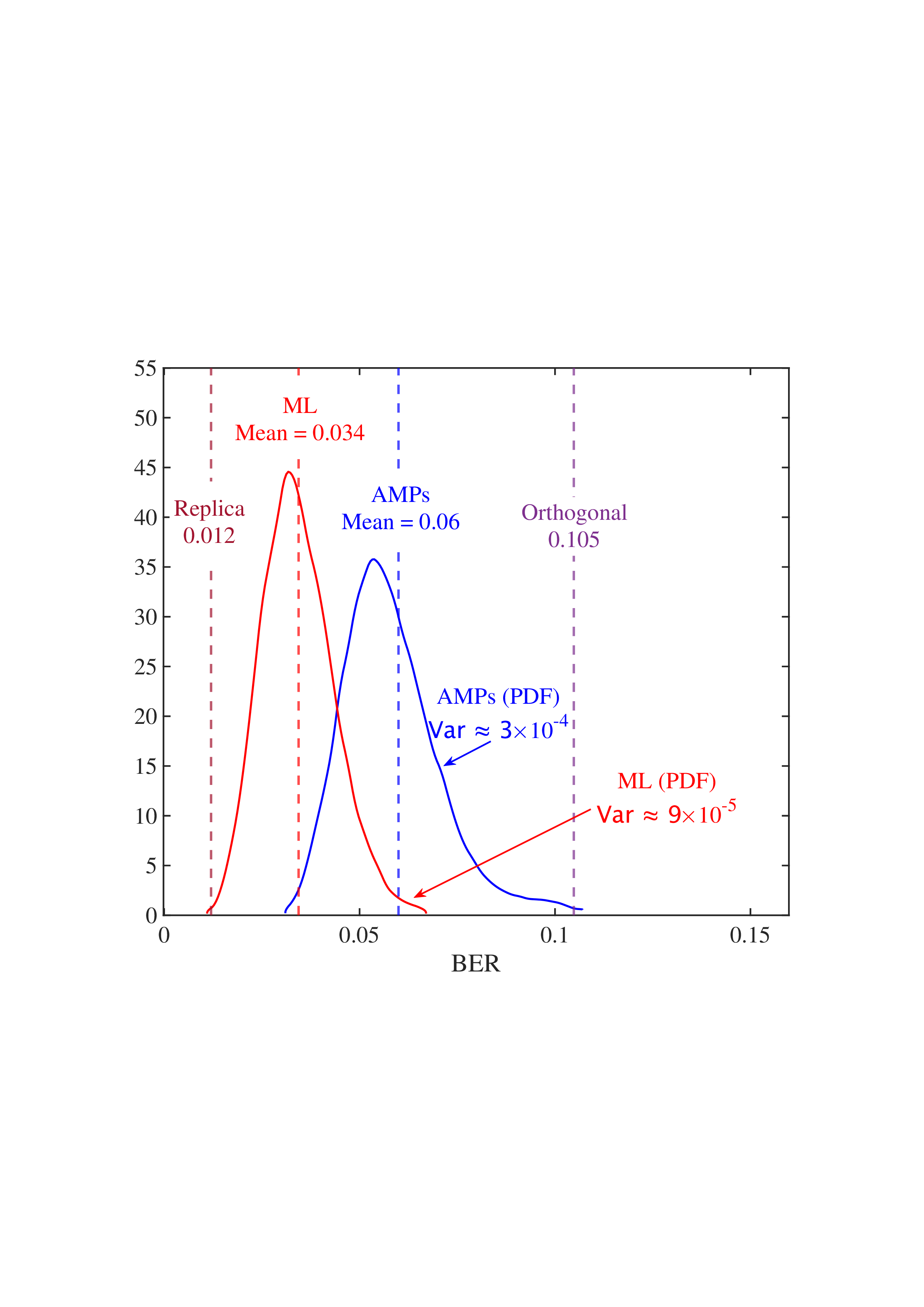
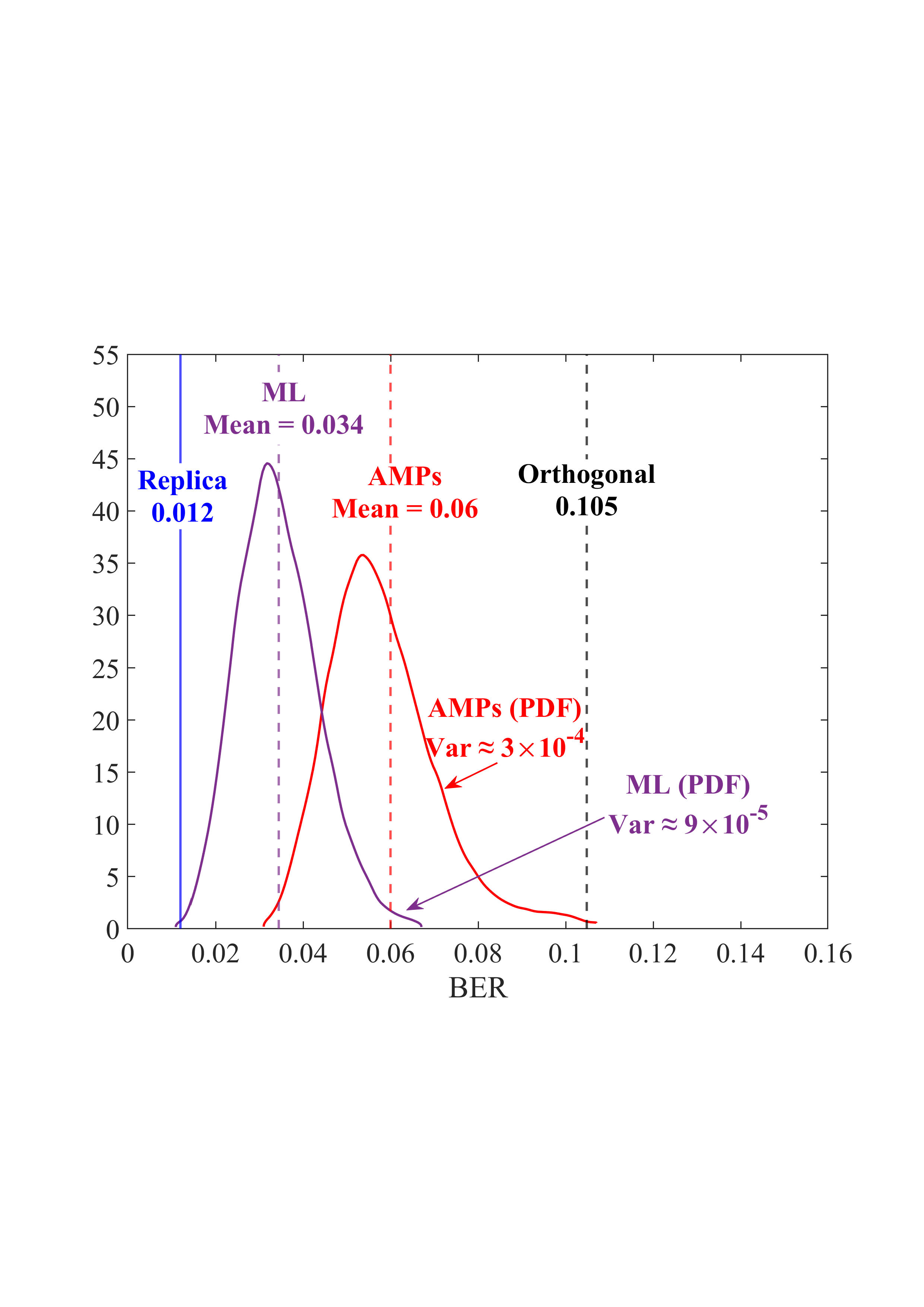
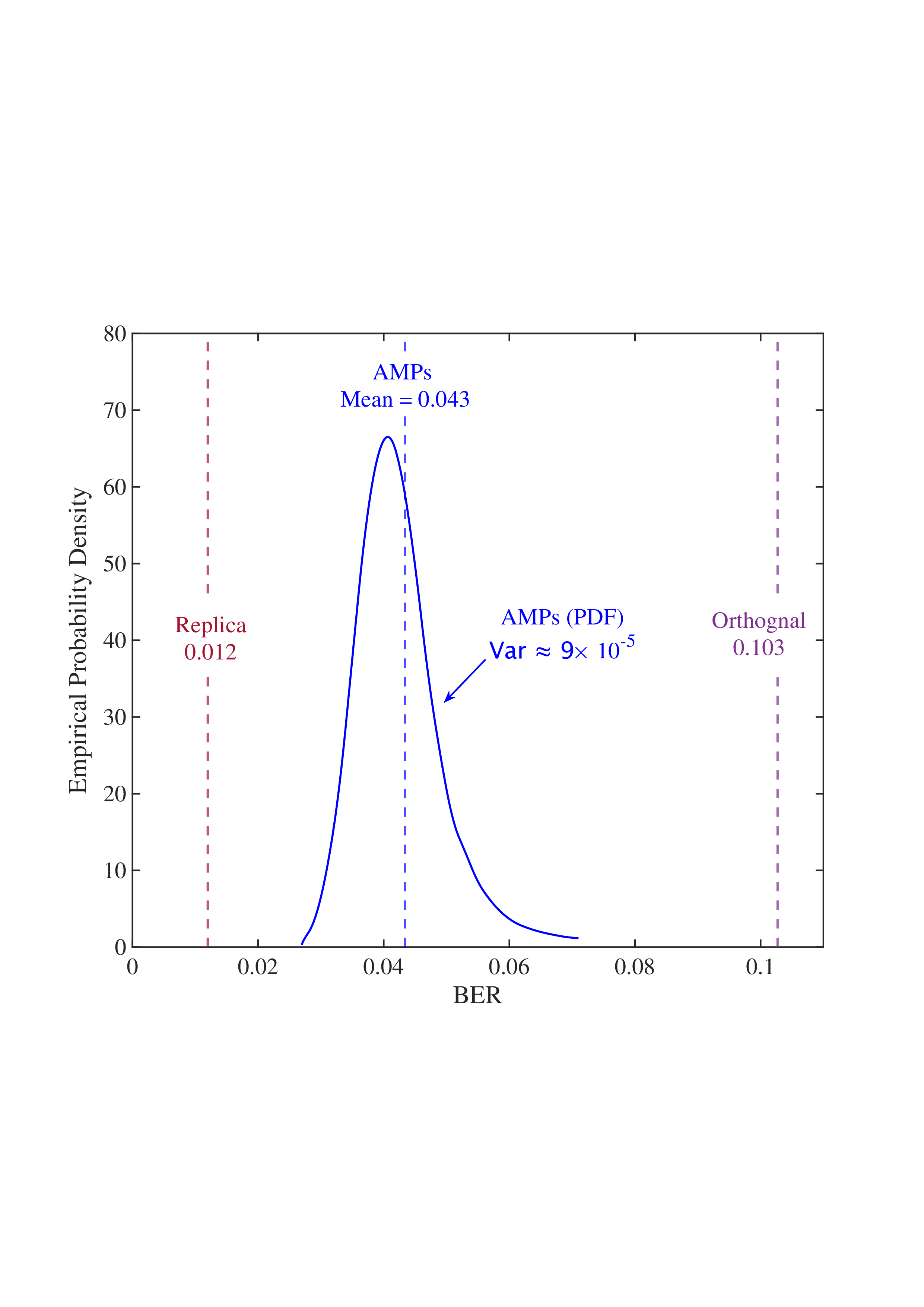
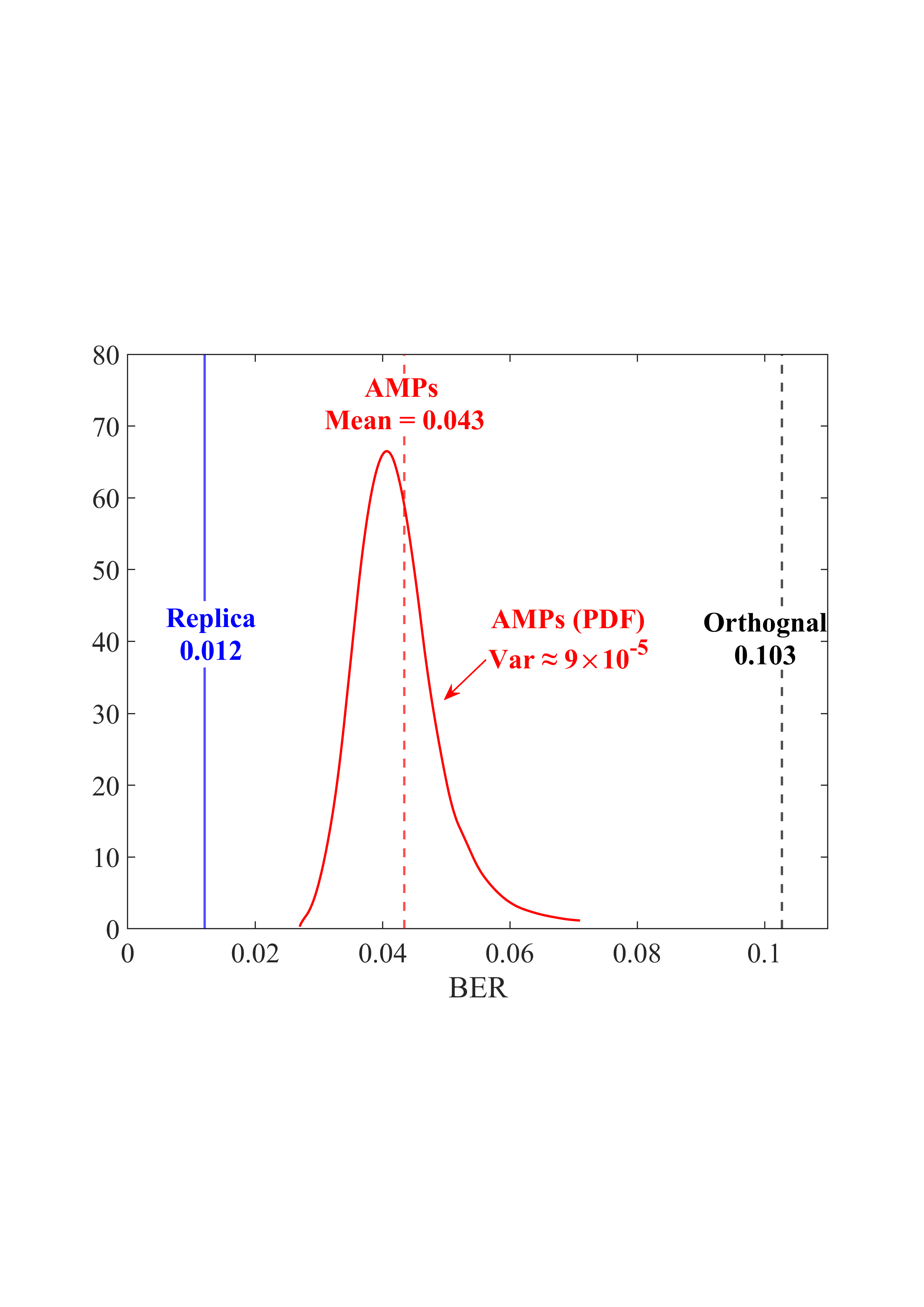
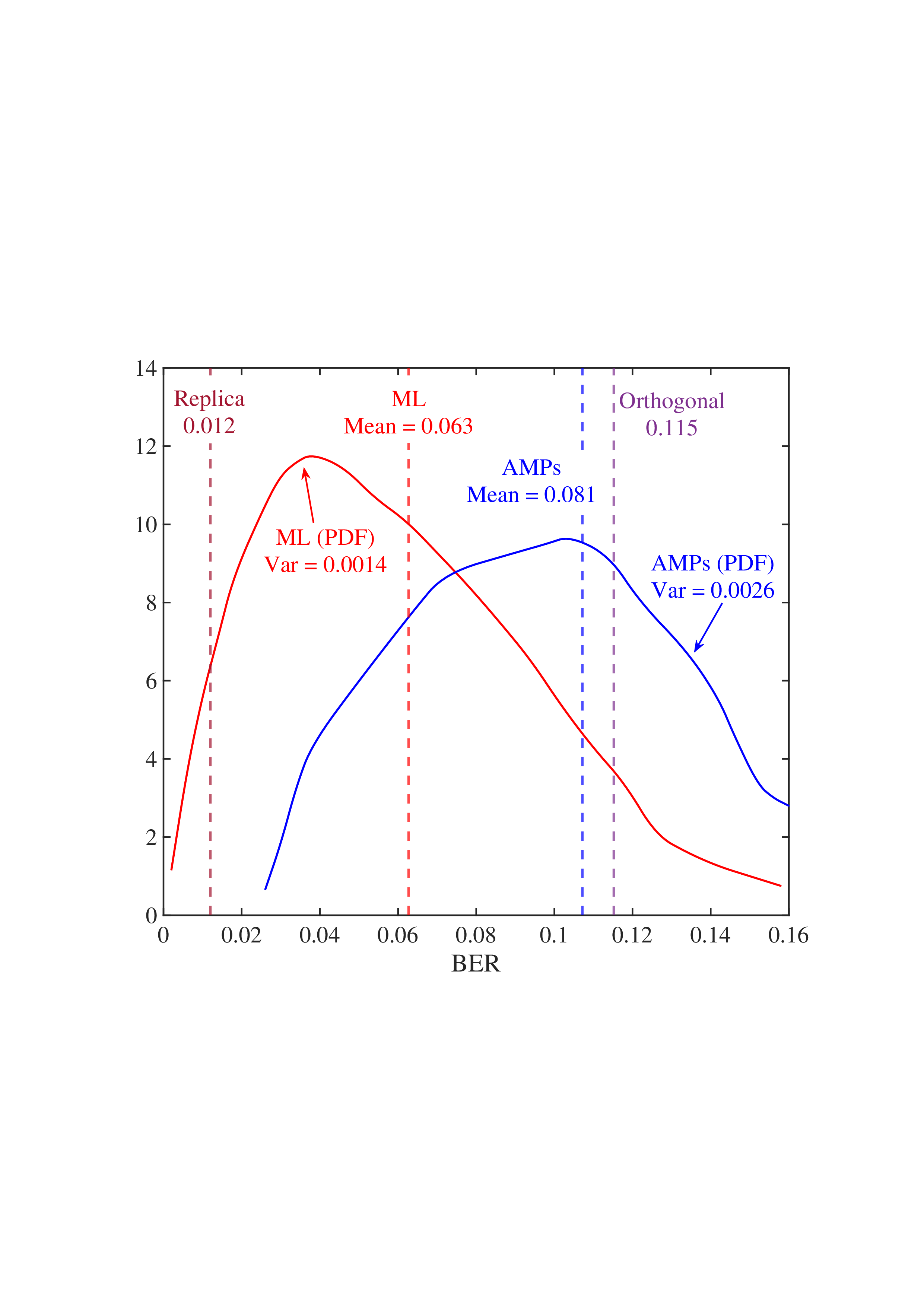
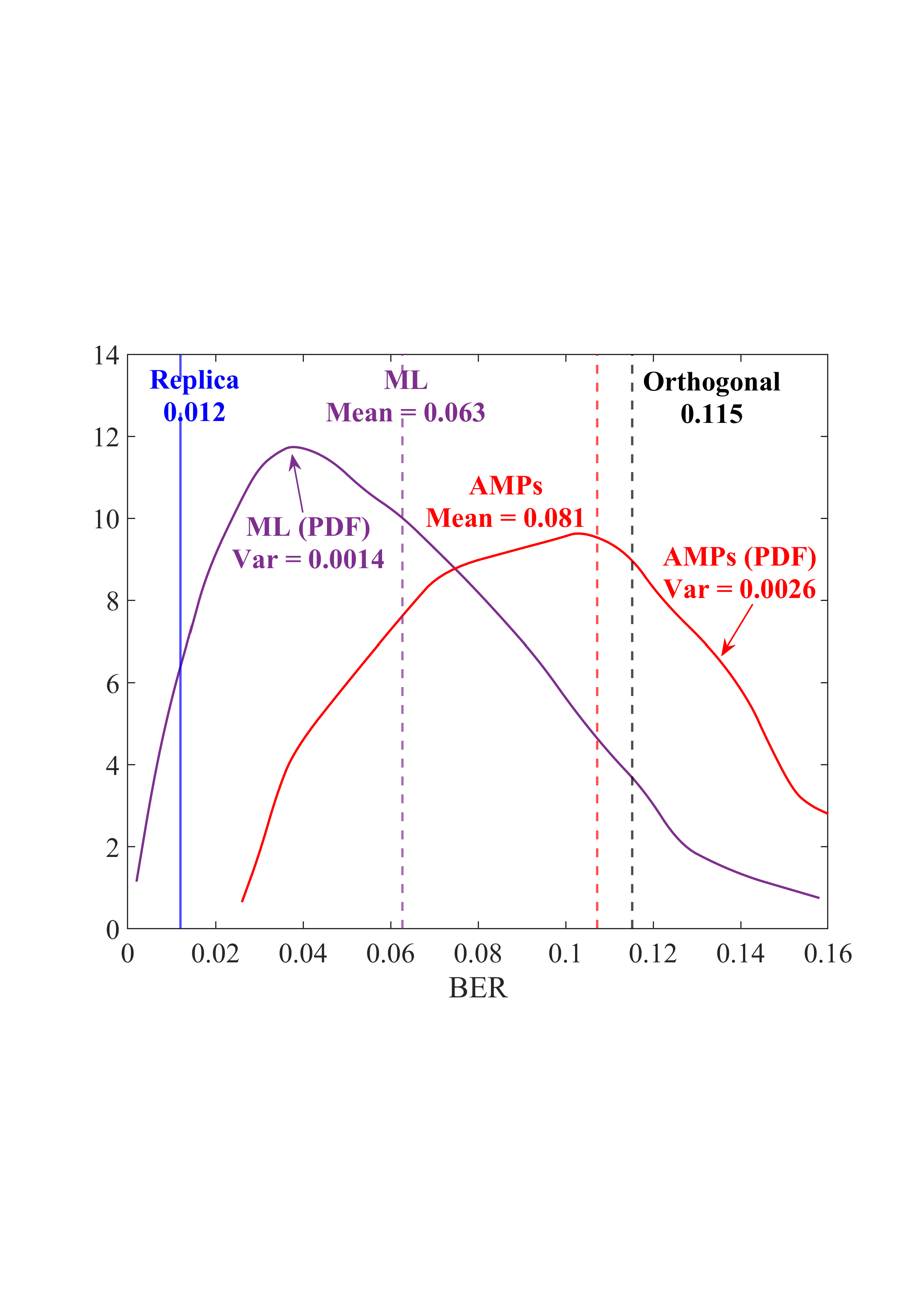
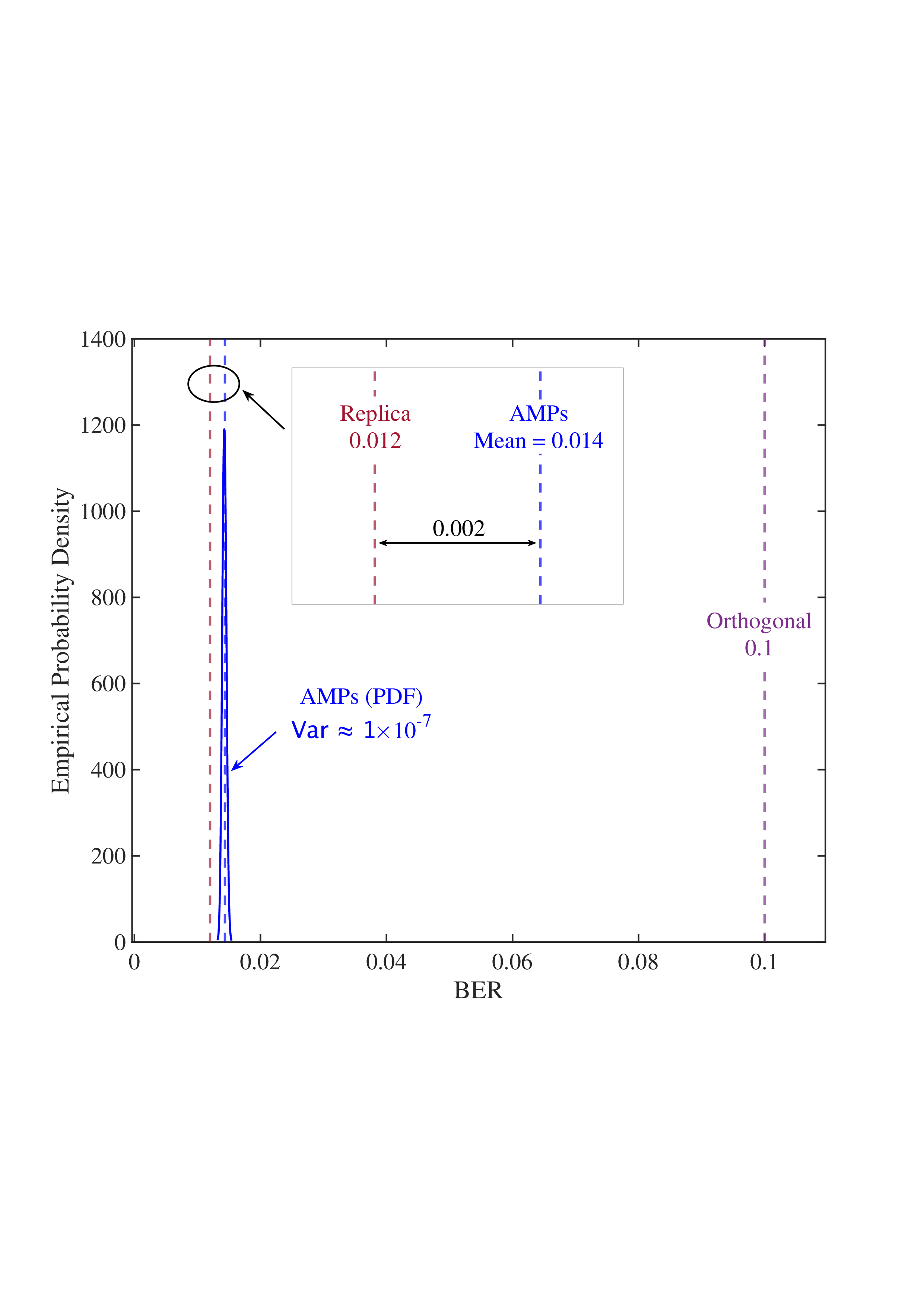
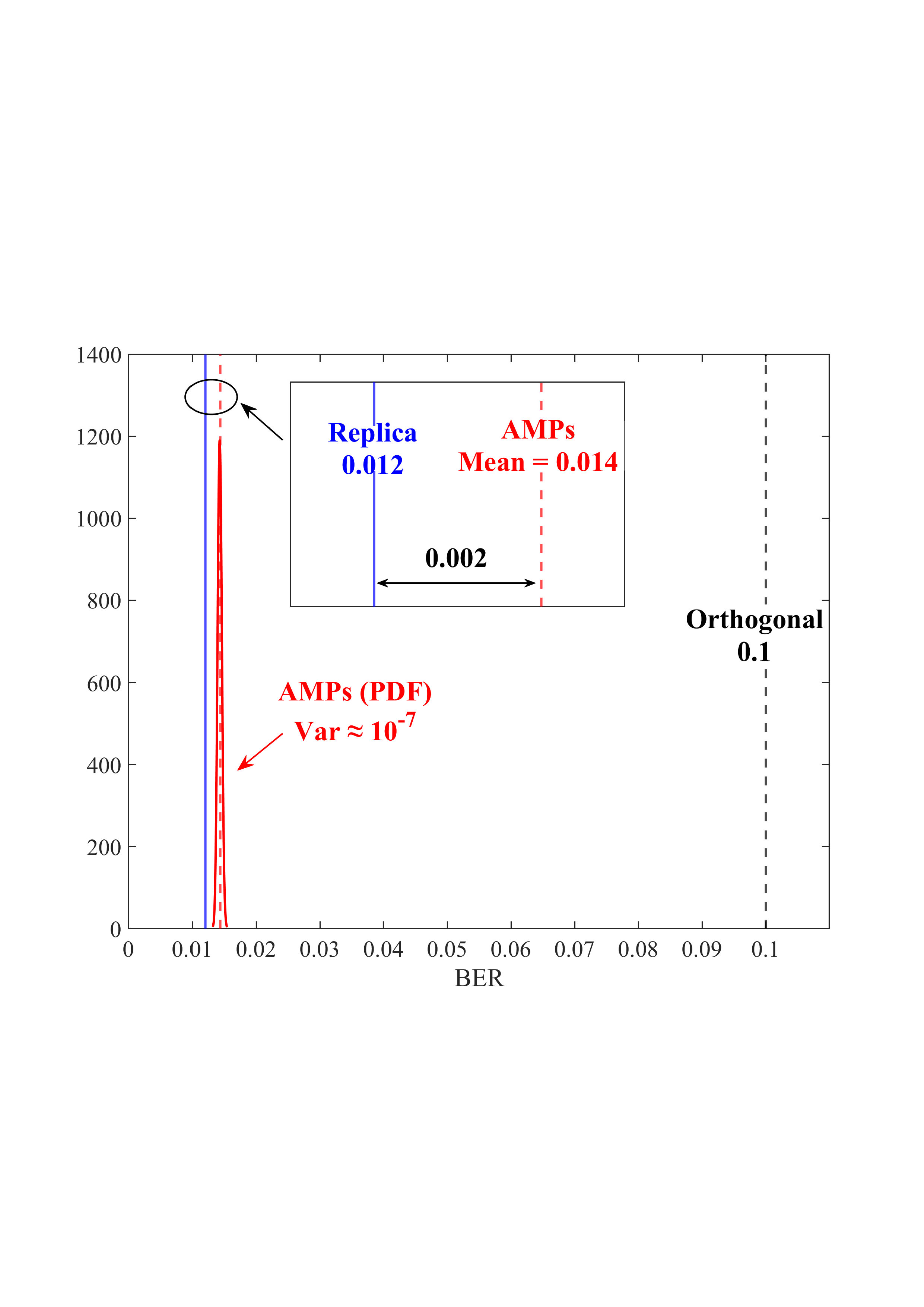
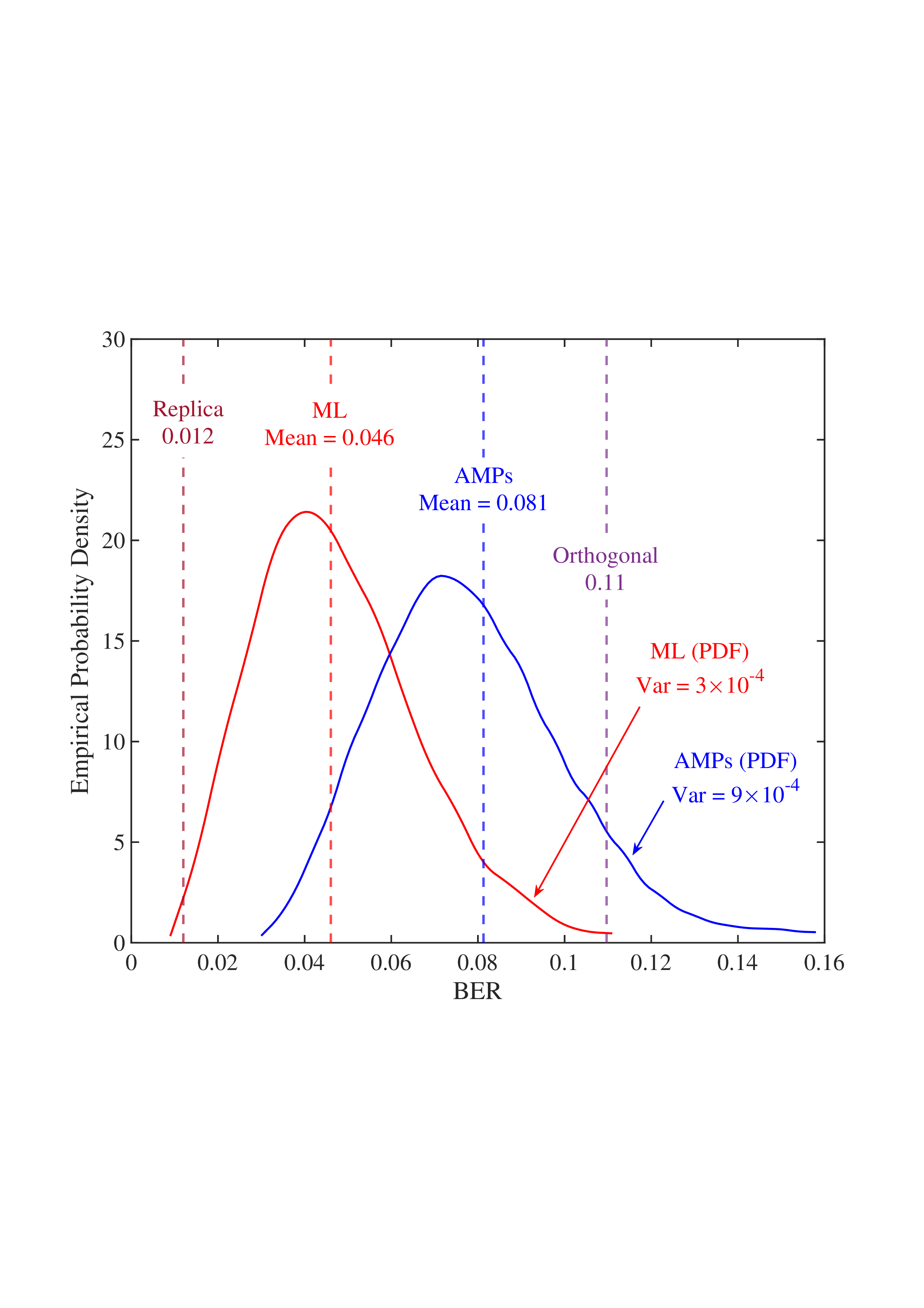
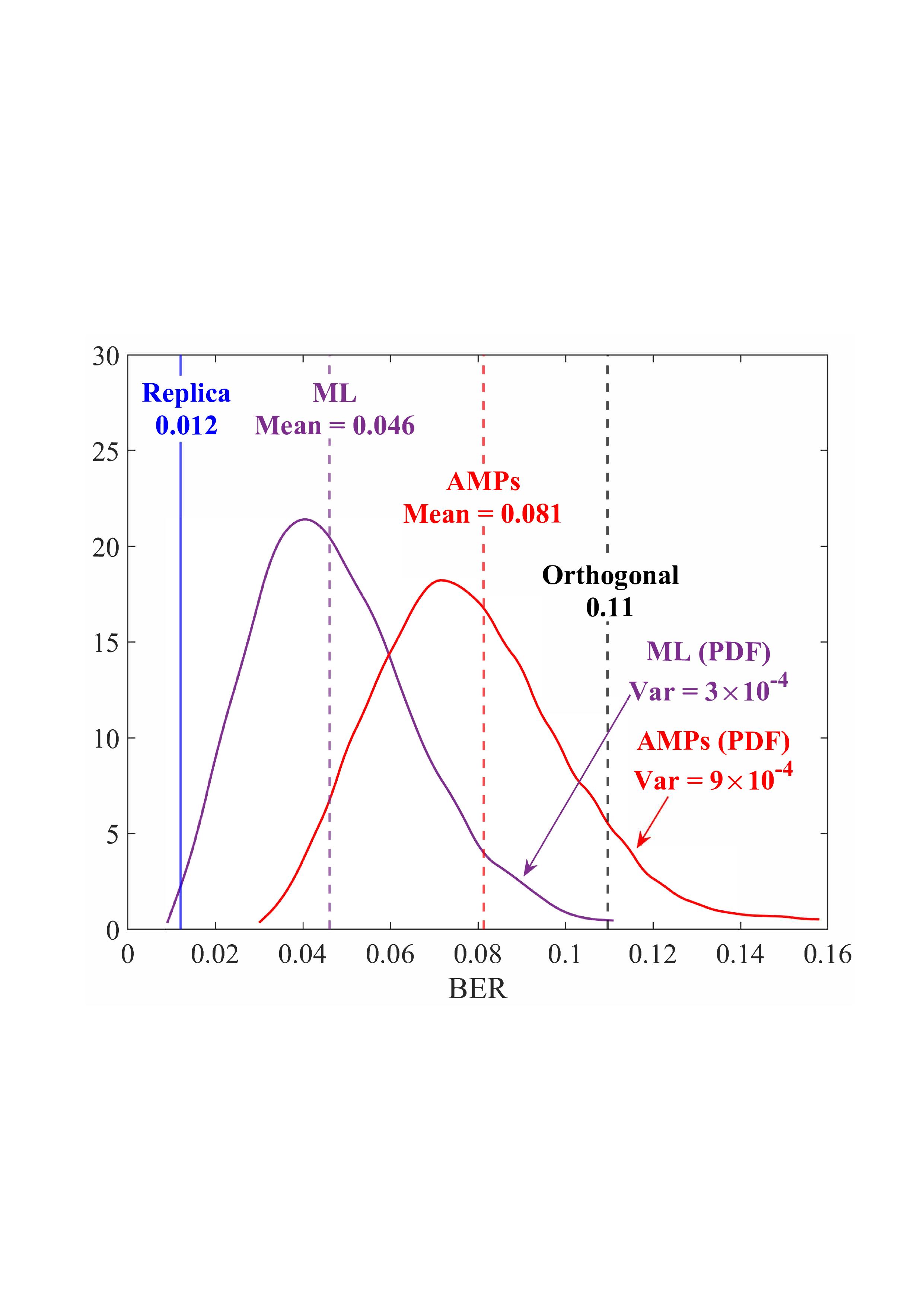
2. Example 2: We compare orthogonal and unitary modulations to study the impacts of a randomly chosen Ξ in highdimensional situations, in which Ξ = V A is set for orthogonal multiplexing and 10 5 RT matrices Ξ are randomly generated3 for unitary multiplexing. As illustrated in Fig. 4, the following trends emerge as the system size increases.

• Replica MAP BER: Based on Lemma 1, “Replica” denotes the average BER performance limit predicted by the replica method for the linear systems. • Converged BER Distribution: For the vast majority of unitary matrices, the BERs of the low-complexity AMP detector are concentrated near its mean. • Near-Optimality of AMP: The BERs of the AMP detector of the random multiplexing approach the replica limit, with the average performance of the AMP detector being (c) N = 512

Fig. 4: BER comparisons for 1) orthogonal multiplexing y = ΣAx + n using an element-wise MMSE detector, 2) unitary multiplexing y = ΣAΞx + n using ML and AMP-type detectors. The ΣA and Ξ = V H A are obtained from the SVD on 10 5 normalized IID Gaussian matrices A. For each A, the BER is averaged over 10 4 Monte Carlo simulations for each detector. The system dimension is set to N ∈ {8, 32, 512}. 0.014, close to the replica limit of 0.012, with only a negligible distance of 0.002.

• ML Performance: Due to the prohibitive computational complexity of the ML detector, the BER curves for the ML detector are not provided for N = {32, 512}. However, its performance is bounded between the replica limit and the performance of the AMP detector. As N increases, AMP approaches ML and then approaches the replica limit. • Poor BER of Orthogonal Multiplexing: The BERs of orthogonal multiplexing with MMSE detection are poor, with marginal improvement as N grows.

In conclusion, the above observations demonstrate that the BER performance of linear systems with randomly generated unitary matrices, when paired with ML or AMP-type detectors, approaches the replica limit with high probability as N increases. That is, as long as the system is sufficiently large, the probability of a randomly generated unitary matrix being good (approaching the replica limit) is extremely high. This effectively solves the difficulty of finding good unitary multiplexing matrices in high-dimensional systems.

Beyond the intuitive explanation above, theoretical analyses have demonstrated that random multiplexing achieves both the replica minimum MSE/BER and the constrained capacity in linear systems [10]- [12], [14], [15], [27], [28], [33], [59]. Refer to Lemma 6 in Section III-C for more details. It is important to note that the replica optimality established in [10]- [12], [14], [15], [27], [28], [33], [59] relies on the assumption that A is right-unitarily invariant, which does not hold for practical channel matrices. This assumption is relaxed through the random multiplexing technique in this paper.

Discussions: The essence of random multiplexing aligns with the random codebook selection in Shannon’s capacity theorem [20]. In high-dimensional systems, a randomly selected codebook is asymptotically capacity-achieving, while welldesigned codebooks often underperform in practice. Unlike random coding, which suffers from the absence of efficient optimal decoding algorithms, the transmitted signals in the linear system with random multiplexing can be effectively recovered using low-complexity AMP-type algorithms.

Signal detection in the linear systems with random multiplexing presents a significant challenge. In this section, we introduce a general cross-domain message passing detection framework, featuring two Bayes-optimal detectors: CD-OAMP/VAMP for theoretical analysis and CD-MAMP for practical low-complexity implementations. Critically, random multiplexing ensures the transform-domain channel matrix exhibits the requisite input isotropy, placing it in the universality class U [36]-a necessary condition for the efficacy of both detectors.

We rewrite the random multiplexing in (11) as

Nonlinear constraint Φ :

The goal is to find the MMSE estimate of s. That is, its MSE converges to [60] mmse{s|y, A, Ξ, Γ,

where ŝpost = E{s|y, A, Ξ, T, Γ, Φ} is the a-posteriori mean of s. In the special case where s is Gaussian, the standard LMMSE detector achieves optimality. However, for arbitrary non-Gaussian s and general A, finding the optimal solution is generally NP-hard [61].

Existing linear detectors, such as ZF and LMMSE, are suboptimal as they ignore the a priori information of the signal s. For this reason, nonlinear iterative detectors, such as the factor graph-based message passing algorithms, are

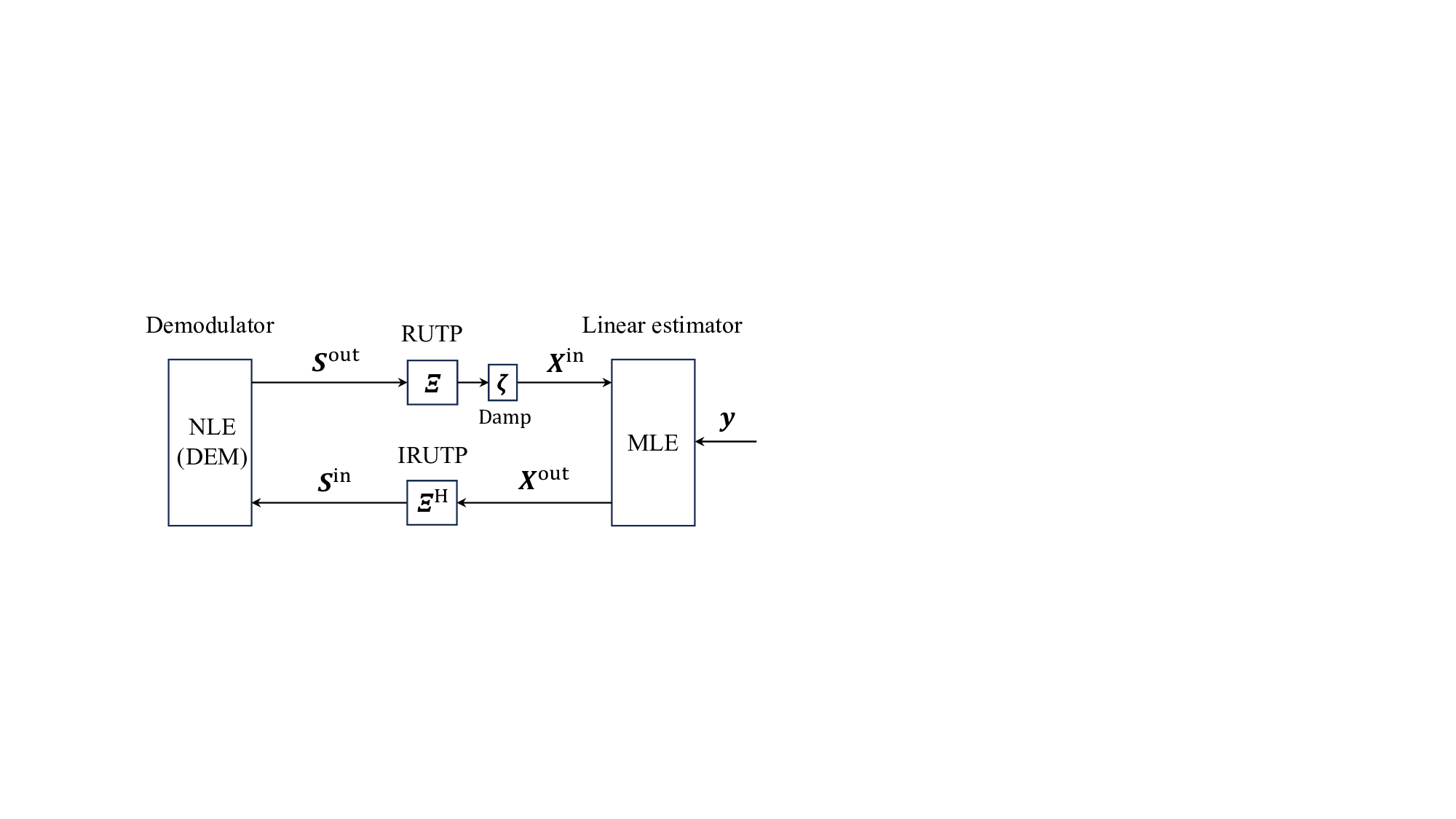
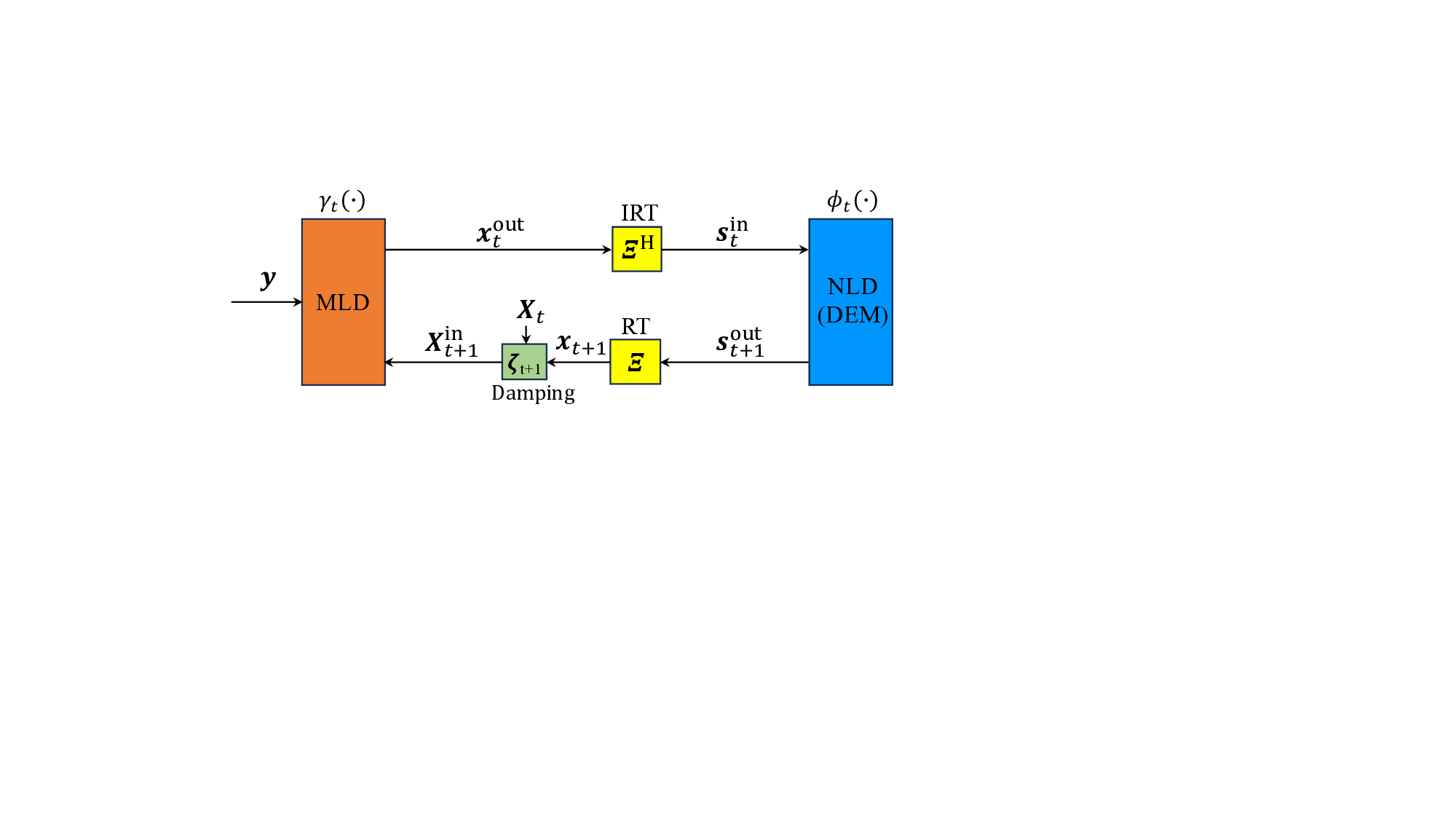
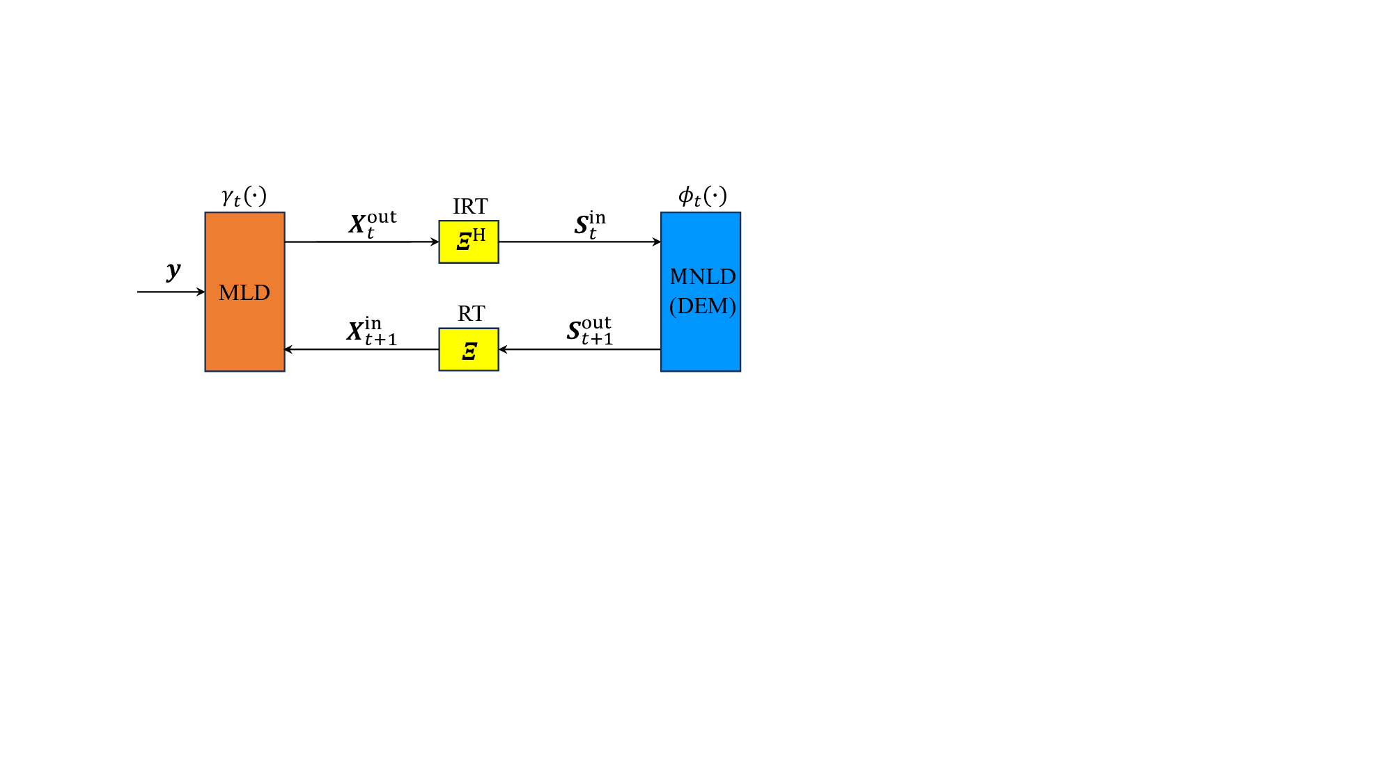
Fig. 5: The CD-MAMP framework for the linear system with random multiplexing, where t denotes the iteration index, Ξ the RT, Ξ H the IRT, and DEM the demodulation.

widely employed [62]. Nevertheless, when the measurement matrix A is dense, it often induces correlation problems, leading to performance degradation. To overcome this limitation, a sequence of advanced AMP-type algorithms, including OAMP/VAMP [10], [11], CAMP [27], long-memory AMP [28], PCA initialized AMP [59], WS-CG-VAMP [33], and MAMP [12], have been developed. In particular, a necessary condition for these algorithms to achieve the replica MAP BER is that the equivalent channel matrix AΞ exhibits sufficient input isotropy (i.e., belongs to the universality class U [36]). However, the wireless channel matrices or the equivalent channel matrices in existing multicarrier systems (e.g., OFDM [1], OTFS [7], and AFDM [8]) exhibit strong structural properties. This discrepancy often leads to significant performance degradation of AMP-type algorithms in practical scenarios. Random multiplexing is a simple yet effective solution to ensure that AΞ exhibits sufficient input isotropy, thereby allowing AMP-type algorithms to achieve the replica optimality under Assumptions 1 and 2.

The CD-MAMP framework and its state evolution (SE) are presented for random multiplexing systems as follows, generalizing the approach in [12], [17].

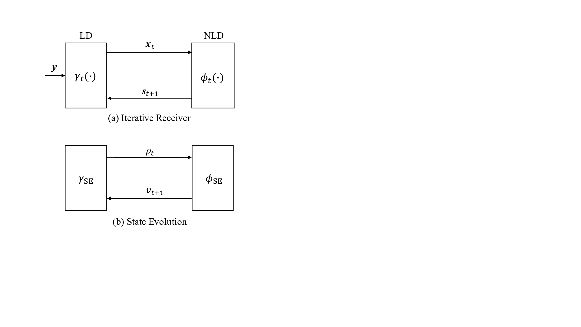
1. CD-MAMP Framework: As shown in Fig. 5, the CD-MAMP detector consists of a memory linear detector (MLD) γ t (•), the random transform (RT) and its inverse (IRT), and a memory nonlinear detector (MNLD) ϕ t (•), which correspond to the linear constraint Γ, the RT T , and nonlinear constraint Φ in (18), respectively. Specifically, MLD is designed to fully exploit the sparsity of the time-domain channels for low-complexity recovery of the time-domain signal x, while MNLD is tailored to incorporate the a priori information of the symbol-domain signal vector s. Then, an iterative refinement process is performed between MLD and MNLD via the RT and IRT, culminating in the recovery of the signal s. A key feature of both MLD and MNLD is the use of orthogonalization to ensure that the input and output estimation errors remain orthogonal. This prevents error correlation during iterative processing. The detailed formulation of the CD-MAMP framework is presented below.

Starting with iteration index t = 1 and X in 1 = 0, MLD :

IRT :

MNLD :

RT :

where 1 N tr Q t A = 1, and tr P t,t ′ = 0, t ′ = 1, . . . , t. (21) We assume that the norms of Q t and P t are finite. Thus, γ t (•) is Lipschitz-continuous. Furthermore, we assume that ϕ t (•) is Lipschitz-continuous and divergence-free, i.e.,

which ensures the orthogonality in MNLD.

2. State Evolution (SE): Suppose that Assumption 1 holds. For the system with random multiplexing in (11), the asymptotic IID Gaussianity result presented in [36, Theorem 3] (along with closely related earlier works in [12], [27], [63]) allows us to evaluate the output covariances of γ t (•) and ϕ t (•) in ( 20) by the SE functions given by: As N → ∞,

where X = x • 1 T and S = s • 1 T with 1 denoting an all-ones vector of proper size, (20). Hence, we rewrite the SE of CD-MAMP in (23) as: Let

The SE provides a methodology for analyzing and optimizing CD-MAMP receivers, characterizing fundamental performance limits such as achievable rates, MAP BER, and constrained capacity. Beyond theoretical analysis, SE plays a pivotal role in system design by facilitating optimal power allocation, guiding channel coding strategies, and demonstrating the constrained-capacity optimality of CD-MAMP receivers.

The CD-OAMP/VAMP detector is proposed in [38], [39] that can be regarded as a special case of CD-MAMP framework, i.e., the current output estimates of γ t (x in t ) and ϕ t (s in t ) in (20) (NLD) [10]. The detailed process is as follows: Starting with t = 1 and x in 1 = 0, LD :

IRT :

NLD :

RT :

where {ϵ γ t , ϵ ϕ t+1 } denote the orthogonalization parameters, i.e.,

and

Based on ( 24) and ( 25), the SE of CD-OAMP/VAMP is single-input single-output based on scalar variances, i.e., LD:

NLD:

This scalar SE plays a critical role in the theoretical analysis of random multiplexing systems. Nevertheless, the sparsity of the time-domain channel matrix H is not effectively used in CD-OAMP/VAMP due to the matrix inversion in (25g), resulting in high complexity and restricting their application in large-scale systems. The low-complexity CD-MAMP detector provides an effective solution to this limitation.

Following the CD-MAMP framework in (20), a CD-MAMP detector is proposed as illustrated in Fig. 6. To avoid the prohibitive complexity of matrix inversion in (25g), particularly in large-scale systems, we adopt a low-complexity memory matched filter rt as an efficient alternative for estimating the time-domain signal x. The detailed process is as follows: Starting with t = 1, x in 1 = 0 N and r0 = 0 M , MLD :

IRT :

NLD :

RT :

Damp :

where rt = B t rt-1 + ξ t (y -Ax in t ), B t = θ t (λ † I -AA H ) with λ † = [λ max + λ min ]/2, λ min and λ max denote the minimal and maximal eigenvalues of AA H , respectively. The parameters {ϵ γ t , p t,i } ensure the orthogonality of input and output errors according to (21) and (22), while {ζ t+1 , θ t , ξ t } are optimized to ensure the convergence or enhance the convergence rate of CD-MAMP. For more details, refer to [12].

Lemma 7 (Asymptotic IID Gaussianity [36]). Suppose that Assumption 1 holds. The asymptotic IID Gaussianity in (23) holds for the CD-MAMP detector in (27) when applied to random multiplexing systems.

Remark: Ref. [36] extends the asymptotic IID Gaussianity of OAMP/VAMP to matrices in a general universality class, while [12] demonstrates that MAMP satisfies the same asymptotic IID Gaussianity conditions as OAMP/VAMP. As a result, for matrices in the universality class, both OAMP/VAMP and MAMP exhibit rigorous state evolution and are replica optimal. Furthermore, CD-MAMP and MAMP are mathematically equivalent, differing only in implementation: CD-MAMP performs memory linear estimation in the time domain to leverage channel sparsity, whereas MAMP operates in the random transform domain. Consequently, the asymptotic IID Gaussianity, state evolution and replica optimality that hold for MAMP also apply for CD-MAMP.

By Lemma 7, the MSE performance of CD-MAMP can be tracked using the SE in (24). However, the high-dimensional covariance matrices V γ t and V ϕ t in ( 24) complicate direct application in performance analysis and optimization. This challenge is addressed by the following lemma, which establishes the fixed-point consistency between CD-MAMP and CD-OAMP/VAMP. This lemma simplifies the complex covariancebased SE analysis of CD-MAMP by using the scalar variancebased SE of CD-OAMP/VAMP in (26).

Lemma 8 (Fixed-Point Consistency [12]). Let the SE fixed point of CD-MAMP in (27) Following Lemma 8, the lower-complexity CD-MAMP can be employed for practical signal detection, while the scalar SE of CD-OAMP/VAMP in (26) can be utilized for the performance analysis and optimization. Since CD-OAMP/VAMP (or CD-MAMP) aligns with that of OAMP/VAMP (or MAMP), the following corollary, derived from Lemma 6, establishes the replica MAP-BER optimality of CD-MAMP in systems with random multiplexing.

Corollary 2 (Replica MAP-BER Optimality). Suppose that Assumptions 1 and 2 hold. For the linear systems with random multiplexing, i.e., AΞ ∈ U , both the CD-OAMP/VAMP detector in (25) and the CD-MAMP detector in (27) can achieve the replica MAP BER in (6).

To demonstrate the advantages of CD-MAMP in complexity, we present a comparison with existing state-of-the-art detectors, in which the measurement matrix A is assumed to be sparse and the number of non-zero elements per row in A is K (K ≪ min{M, N }), e.g., time-varying multipath channels [1], etc. For CD-MAMP, AA H rt and A H rt in (27a) are dominated and their time complexity is O(KM T ), where the maximum iteration number T ≪ N . In addition, Ξ can generally be implemented using a random interleaver and fast transformation matrices, such as DFT or Hadamard-Walsh transform matrices, with a time complexity of O(N logN ). The space complexity of CD-MAMP is O(KM ) to store the non-zero elements of A, O (M + N )T for {x t , x in t , x out t } and {s in t , s out t }, and O T 2 for associated covariance matrix (see details in [12]). Since Ξ can be constructed from an interleaver and a structured transform matrix (e.g., DFT or DCT), its fast algorithm avoids explicit storage. Table I presents the comparisons in time and space complexity of CD-MAMP, CD-OAMP/VAMP [19], [38], [39], symbol domain (SD) MAMP [41], SD Gaussian message passing (GMP) [62]. Hence, CD-OAMP/VAMP, SD-GMP, and SD-MAMP have higher complexity than CD-MAMP for T ≪ N and K ≪ min{M, N }.

V. POWER ALLOCATION Generally, the base station can acquire channel state information (CSI), while low-cost transmitters face difficulties in obtaining perfect CSI directly. To address this challenge, CSI feedback has been widely studied as a means to transmit accurate CSI from the base station to the transmitter [64]. In this section, we assume that CSI is available at both the transmitter and receiver. We investigate optimal power allocation strategies for the linear system with random multiplexing, aiming to minimize the MAP BER and maximize the constrained channel capacity, respectively.

In this section, we study the RT-domain power allocation in linear systems with random multiplexing, given by y = HP Ξs + n,

where P ∈ C N ×N is a power allocation matrix subject to tr{P P H } = P sum (total transmit power).

Theorem 2 (Optimal Power Allocation Matrix). Let H = U H Σ H V H H be the singular value decomposition of H. Then, regardless of whether the objective is to minimize the MAP BER or to maximize the constrained capacity of the asymptotic system in (28), the optimal form of P is

where

be optimized, and V P is an arbitrary unitary matrix. For simplicity, and without loss of generality, we can set V P = I so that

Proof: In [19], it was proven that ( 29) is optimal for minimizing P sum under a given MAP BER. We show that ( 29) is optimal for both minimizing the MAP BER and maximizing the constrained capacity under a given P sum . Our proof employs an intermediate result in their proof. See Appendix E for details.

Following Theorem 2, we reformulate (28) as

where Σ H = diag{σ 1 , . . . , σ min(M,N ) } is an M × N rectangular diagonal matrix. The power allocation reduces to

The intuitions are as follows.

• The RT matrix Ξ enhances the input isotropy of the equivalent channel matrix. • The unitary matrix V H enables us to diagonalize the channel matrix H. • The power allocation matrix Σ P optimizes the singular values of the equivalent channel matrix, thereby significantly improving the MAP BER or the constrained capacity of the systems. According to Theorem 1, HV H Σ P Ξ belongs to the universality class U . This leads to the following corollary.

Corollary 3 (Replica MAP BER Optimality). Suppose that Assumptions 1 and 2 hold. The replica MAP BER of the random multiplexing system in (31) can be achieved by both the CD-OAMP/VAMP and CD-MAMP detectors in Section IV when substituting A with HV H Σ P under the optimal power allocation vector p * .

Remark: One may consider the symbol-domain power allocation, where the signal undergoes power allocation before being transmitted through multiplexing with Ξ, given by y = HΞΣ P s + n.

In this case, unequal power allocated coefficients amplify the asymmetry among the signal elements in s, leading to the severe performance degradation, similar to the orthogonal case shown in Fig. 3(c). This is why we focus solely on the RTdomain power allocation in (31).

For simplicity of discussion, we rewrite (31) as:

where ỹ = U H H y, ΣH = diag{σ 1 , • • •, σ N } with σ i = 0 for min{M, N } < i ≤ N , and ñ ∼ CN (0, σ 2 I). Then, the sate evolution (SE) of CD-OAMP/VAMP for the power allocated linear system is

where

where

, and (a) follows pi ≡ ϱ i p i .

Here, we provide two crucial properties essential for presenting our main results of optimum power allocation in Subsections V-C and V-D.

Lemma 9 (Concavity of 1/γ SE ). The function [γ SE (v, p)] -1 , where γSE (•) is given in (35), is concave w.r.t. (with respect to) p.

Proof: See Appendix D.

Power allocation to minimize MAP BER is tailored for the receivers employing a MAP detector cascaded by a decoder, without any iteration between the two. In this context, effective SISO-AWGN codes are sufficient for linear systems, rendering channel code optimization unnecessary. As a result, maximizing the achievable rate is equivalent to minimizing the MAP BER at the detection stage.

1. Problem Formulation: Following Lemma 1, the MAP BER of the power allocated linear system in (31) can be evaluated by the following lemma. Lemma 11 (Replica MMSE and MAP BER). The replica MMSE v * of the power allocated linear system in (31) is the unique solution of

where R R (•) is the R-transform with R = Σ H P ΣH H ΣH Σ P . Let ρ * = mmse -1 (v * ) . The replica MAP BER of the power allocated linear system in (31) is

where Q S (ρ) denotes the BER function of MAP demodulation for √ ρx + z given signal constellation S, i.e., x i ∈ S, ∀i, as defined in Appendix A.

Following (37), to minimize the replica MAP BER of the system in (31), the power allocation is formulated as the following optimization problem:

2. Problem Transformation: Since Q S (•) is a monotonically decreasing function, Problem P 1 reduces to

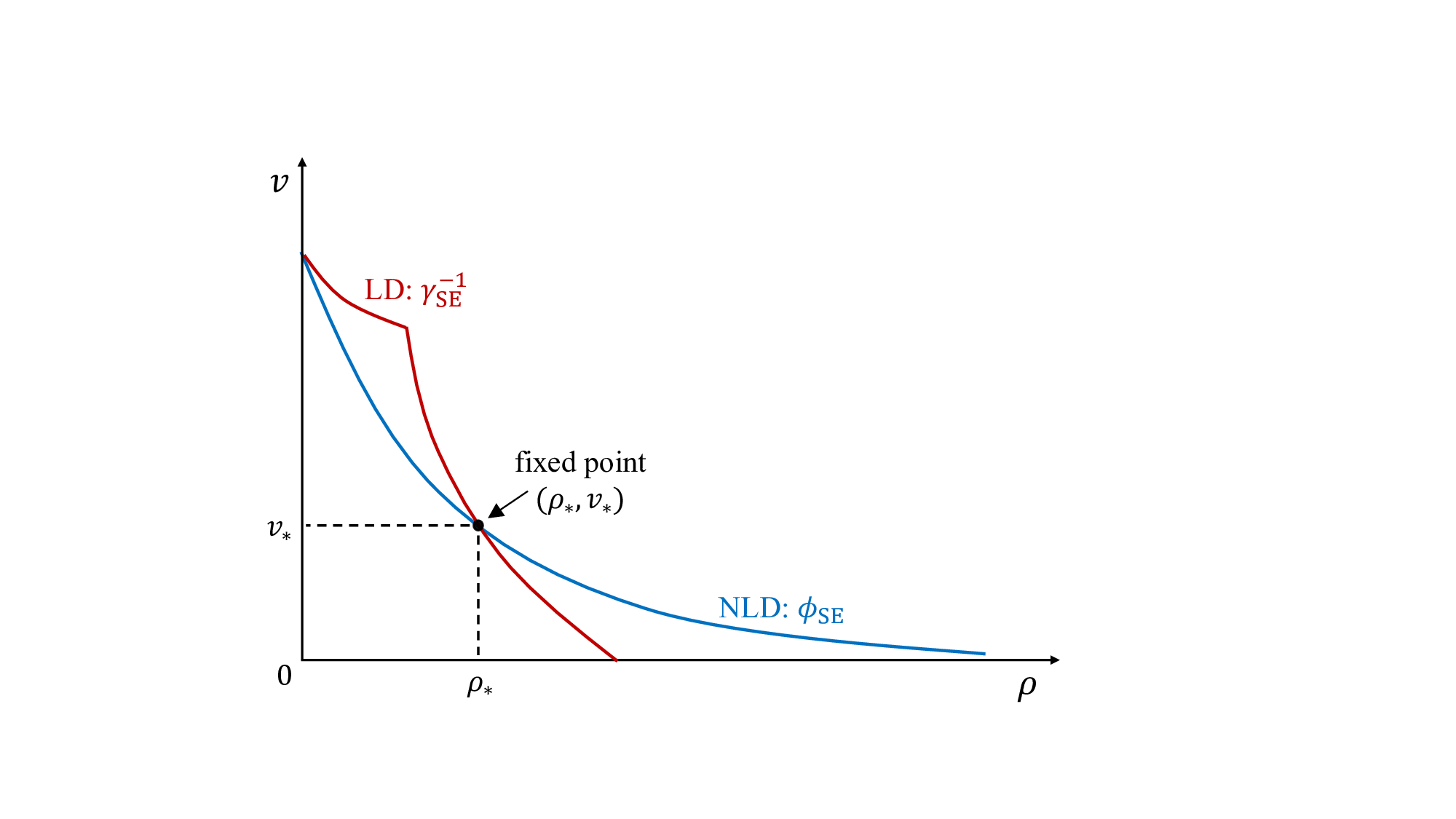
In general, obtaining ρ * by directly solving (39) is challenging. Fortunately, as shown in Corollary 3, CD-OAMP/VAMP can achieve the replica MAP-BER optimality in (31), and its convergence has been established in [12], [34], [35]. Hence, we address this issue by analyzing the first fixed point (ρ * , v * ) of the SE of CD-OAMP/VAMP:

where γ SE (•) and ϕ SE (•) are given in (34). Then, we have

Based on this analysis, Problem P 1.1 can equivalently transformed into a bi-level optimization problem: find v goal ∈ (0, 1) such that P 1.2 (v goal ) = 0, where

For any fixed P sum , P 1.2 (v goal ) is monotonically increasing w.r.t v goal , which can be proven by contradiction. Hence, the unique v goal satisfying P 1.2 (v goal ) = 0 can be obtained via a bisection search. However, it is hard to compute the minimum of γ SE (v, p) -ϕ -1 SE (v) over the continuous interval v ∈ [v goal , 1). To address this issue, we replace it with the minimum over V goal , a discrete set of log-uniformly sampled points within [v goal , 1). In practice, 100 sampling points are typically used, i.e., |V goal | = 100.

In summary, we can solve P 1 numerically by: finding v goal ∈ (0, 1) via a bisection search, such that the corresponding V goal satisfies P 1.3 (V goal ) = 0, where

3. Concavity: The following lemma shows that P 1.3 is a concave maximization problem over a convex set, which is well-known to be equivalent to a convex problem, enabling its solution via standard convex optimization solvers.

Lemma 12. P 1.3 is a concave maximization problem over a convex set.

Proof: It is easy to verify that the constraints of P 1.3 are convex. Hence, we only need to show the concavity of

, the problem reduces to showing the concavity of [γ SE (v, p)] -1 w.r.t. p, which was established in Lemma 9. Thus, we finish the proof.

The search interval is initialized to (0, v up ). Setting v up = 1 is always a natural choice. The iterative process is:

, and obtain the set V i by uniformly sampling on [v i , 1) in log domain.

• Step 2: Find the solution p (i) and the corresponding objective function value c i of P 1.3 with V goal = V i by convex optimization solvers.

In practice, the SE of CD-OAMP/VAMP is not perfectly accurate since the system size is finite. To ensure that CD-OAMP/VAMP converges to its SE fixed point, we revise step 1 and step 3 by introducing a small threshold ϵ > 0:

, and obtain the set V i by uniformly sampling on (v i , 1) in log domain.

The pseudocode is given in Algorithm 1. The stopping threshold ∆ v controls the precision of the output v, and the threshold ϵ serves as a safety margin to account for potential mismatch between the SE and the actual performance of CD-OAMP/VAMP in finite systems. In our simulations, we set ∆v = 10 -6 to ensure ∆v/v ≪ 1. For systems with N = 2048, we set ϵ = 0.45 empirically.

Note: In [19], power allocation is addressed by minimizing the total power under a target MAP BER, formulated as optimizing p to minimize

Get V goal by log-uniformly sampling in (v, 1)

Get p and c by solving

if c > ϵ then 8:

end if 16: end while if 1/γ SE is concave w.r.t p, with the proof, omitted in [19], derived in Lemma 9. Consequently, the problem can be solved by convex optimization solvers. Nevertheless, directly solving P 1.1 in ( 39) is challenging. To overcome this, we reformulate P 1.1 into a bisection search framework based on P 1.3 in (43). Furthermore, we offer practical implementation details, such as discretizing the continuous intervals in the logarithmic domain and introducing a threshold ϵ to account for the inaccuracy of the SE. These measures are essential for solving both the power allocation problem in this paper and the one in [19].

In this subsection, we study the power allocation to maximize the constrained capacity of the power allocated linear system in (31), an issue not addressed in [19].

1. Problem Formulation: The constrained capacity of the system in (31) can be evaluated by the following lemma.

Lemma 13 (Replica Constrained Capacity). The replica constrained capacity per transmit symbol of the linear system in (31) is given by

where R = Σ H P

H ΣH Σ P , ρ * = mmse -1 (v * ), and v * is the replica MMSE given by the unique solution of (36).

To maximize the constrained capacity of the system in (31), the power allocation is formulated as the following optimization problem: where C MIMO (p) is given in (44).

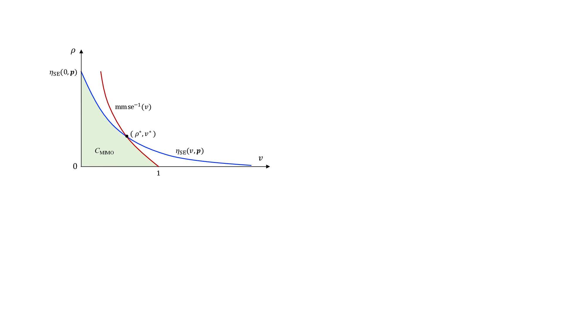
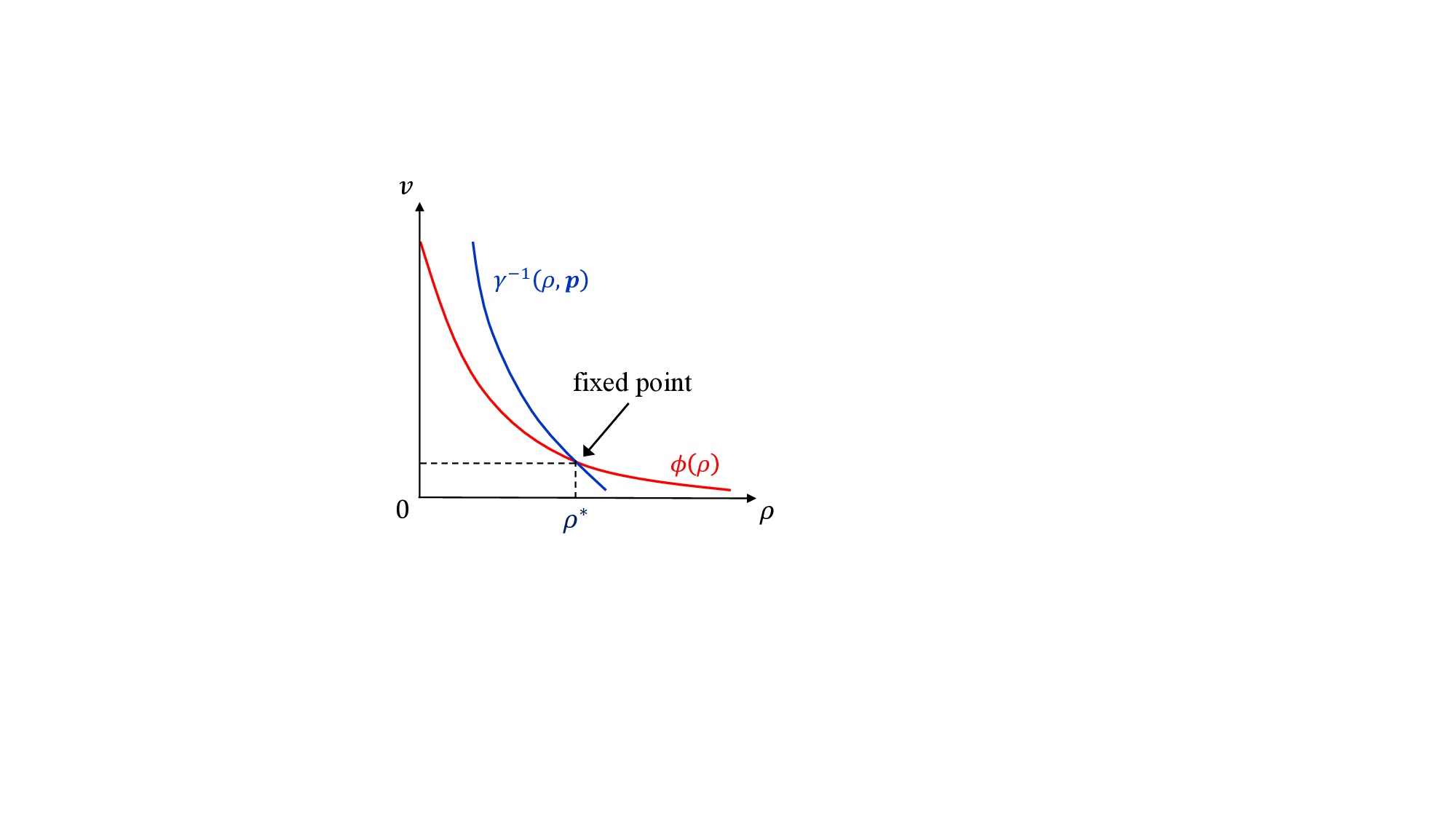
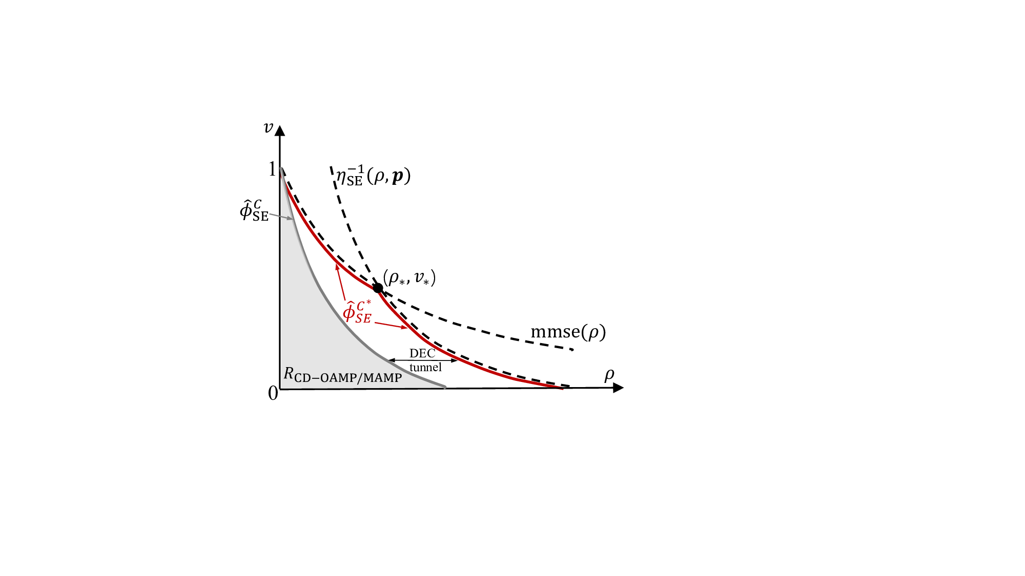
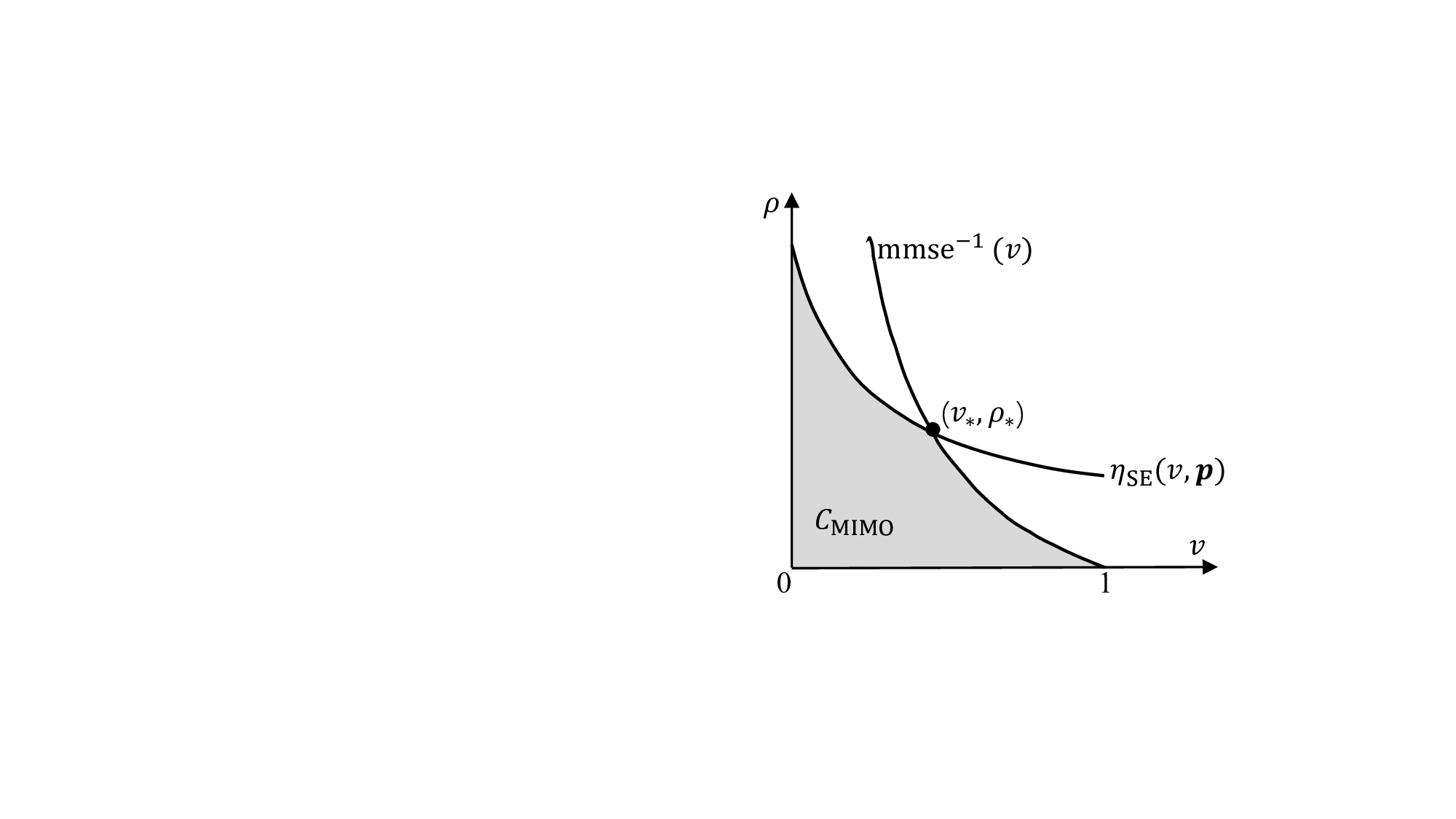
In this case, the optimal power allocation corresponds to the waterfilling solution [21]. Conversely, for non-Gaussian signaling s, the power allocation becomes more complex. Following the capacity-area theorem in [14, Theorem 1], the linear capacity C MIMO in ( 44) can be reformulated to

where η SE (•) is the variational transform function given by

with γ-1 SE (v, p) being the inverse function of v = γSE (ṽ, p) w.r.t. ṽ. Fig. 7 provides a graphic illustration of (46). Note that the ϕ SE (•) in (34b) involves an orthogonalization operation in the SE of CD-OAMP/VAMP, rendering it no longer locally MMSE optimal. This complicates the analysis of constrained capacity and achievable rates using the I-MMSE lemma [56]. This difficulty can be overcame by utilizing the variational transform functions of CD-OAMP/VAMP, as outlined in [14,Equation (37)], preserving the same fixed point as the SE described in (34).

2. Convexity: The following lemma shows that P 2 is a concave maximization problem over a convex set, thus enabling its solution via standard convex optimization solvers. Lemma 14. P 2 is a concave maximization problem over a convex set.

Proof: It is straightforward to verify that the constraints of Problem P 2 are convex. Hence, we only need to show that C MIMO (p) is concave w.r.t. p. Following Lemma 10, [γ -1 SE (ṽ, p)] -1 is convex w.r.t. p. Therefore, η SE (ṽ, p) is concave w.r.t. p. Furthermore, since mmse -1 (ṽ) is independent of p, and the integral operation and the minimum operation both preserve concavity, we obtain that C MIMO (p) is concave w.r.t. p. Hence, we complete the proof of Lemma 14.

3. Numerical Solution: It is intractable to find the closedform expressions of mmse -1 (v) and η SE (v, p). Therefore, we compute them as follows:

where g(v, p) ≡ min η SE (v, p), mmse -1 (v) , and v low > 0 is a small threshold. The term v low g(v low , p) approximates v low 0 g(v, p)dv using a rectangular rule. Typically, setting v low ∈ [10 -4 , 10 -3 ] is suitable. The pseudocode is given in Algorithm 2. The stopping threshold ϵ controls the precision of fun(v, p), thereby determining the accuracy of the integral in C(p). Therefore, ϵ is required to be sufficiently small. In our simulations, we set v low = 10 -4 and ϵ = 10 -15 .

Channel coding is crucial for achieving high-speed, reliable information transmission. Most current studies focus on well- if γSE (ṽ, p) -v < ϵ then else if γSE (ṽ, p) -v > ϵ then end while 15:

return min{η, mmse -1 (v)} 17: end Function designed codes that approach the SISO channel capacity. However, these schemes often neglect inter-symbol interference introduced by the measurement matrix A. Previous research has optimized codes and demonstrated replica constrained capacity for linear systems like (3) under the assumption that the channel A is IID Gaussian [13] or right unitarily invariant [14], [15]. Unfortunately, real-world wireless channels rarely meet this assumption, which limits the applicability of these conclusions. This assumption is relaxed in this paper by random multiplexing, allowing both code optimization and replica constrained capacity optimality hold for arbitrary norm-bounded and spectrally convergent channel matrices. This section introduces the optimal channel coding for the linear system with random multiplexing. CD-MAMP achieve the replica-constrained capacity in random multiplexing systems.

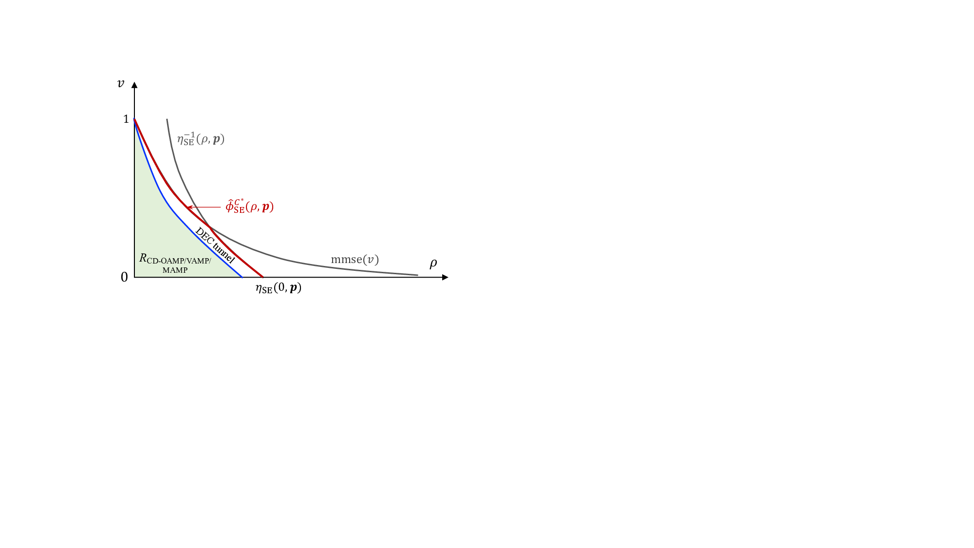
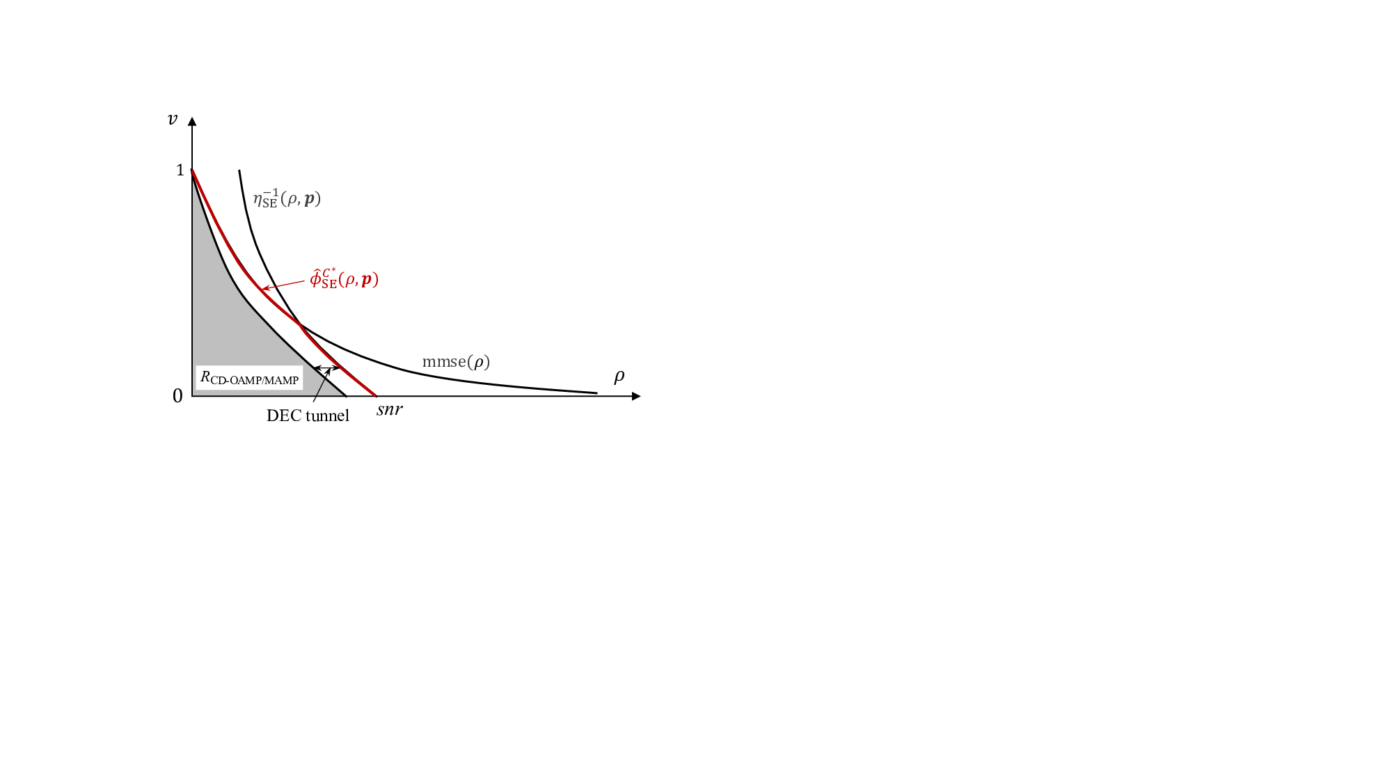
Theorem 3 (Capacity Optimality). Suppose that Assumptions 1-3 hold. When φC SE (ρ) → φC * SE (ρ) = min{mmse(ρ), η -1 SE (ρ, p)}, the achievable rate of the CD-OAMP/VAMP and CD-MAMP receiver per transmit symbol is maximized and expressed as

) which corresponds to the replica constrained capacity of the random multiplexing system, i.e.,

The optimal coding principle in Lemma 17 and the capacity optimality of the CD-MAMP in Theorem 3 are established based on the SE fixed-point consistency in Lemma 8, rather than the consistency of the SE trajectory. This has been proven in [15,Theorem 3], namely, when the channel matrices belong to the universality class, iterative algorithms with the same SE fixed point, such as OAMP, VAMP, and MAMP, share identical rate analysis, optimal coding principle, and capacity optimality. As a result, the codes optimized for CD-OAMP/VAMP are also optimal for CD-MAMP.

In this section, we explore the generality of random multiplexing by highlighting its potential in various common wireless application scenarios.

In practice, it is typical to set the random transform matrix Ξ = ΠF D, where Π is a random permutation, F a normalized fast transform matrix, and D a random phase matrix independent of Π. To guarantee that AΞ ∈ U , the condition in (13) for Theorem 1 is necessary. However, it is hard to claim that practical channel matrices always satisfy this condition. We can even consider an extreme example as:

where Z is an IID Gaussian matrix with Z i,j i.i.d.

∼ CN (0, 1). We have

where the upper bound almost surely converges to 3. Hence, ∥A∥ 2 ≲ 1.

• The empirical spectral distribution of A H A converges to a Marchenko-Pastur distribution supported on [0, 4]. Hence, A is spectrally convergent.

), meaning that it does not satisfy the condition in (13). (1). As a result, AΞ / ∈ U . However, for any spectrally convergent and norm-bounded matrix A, including that in (55), we observe that the performance of OAMP/VAMP with AΞ always matches the SE well in large-scale systems (e.g. N > 1000). This motivates the following conjecture.

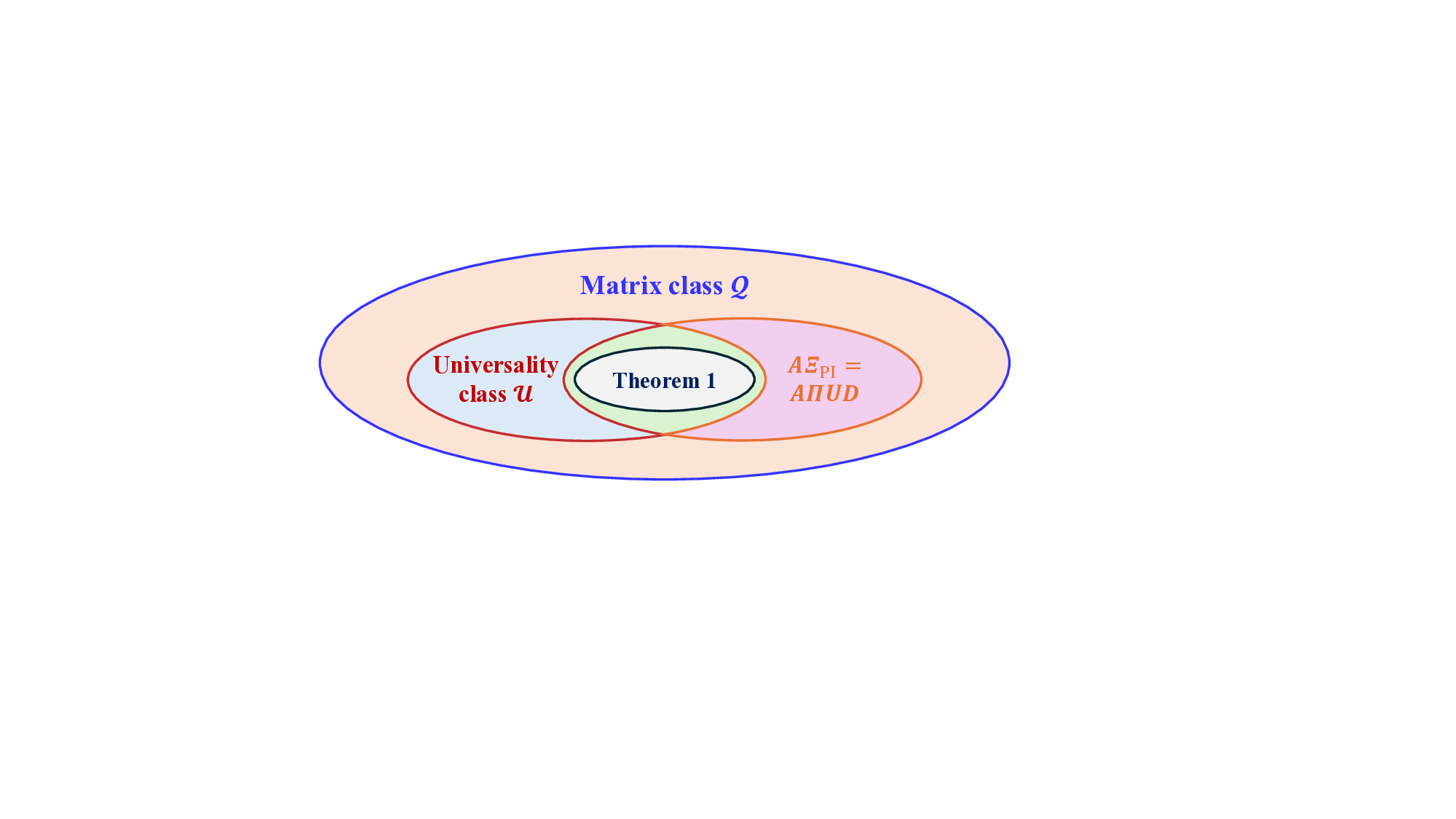
Conjecture 1. There exists a broader matrix class Q, which contains the universality class U (i.e., U ⊂ Q), such that the error vectors in OAMP/VAMP are asymptotically IID Gaussian and thus the SE is accurate. Moreover, for any spectrally convergent A with ∥A∥ 2 ≲ 1, and any Ξ PI defined in Theorem 1, AΞ PI ∈ Q.

To reduce computational complexity and storage requirements, we typically set the random transform matrix as Ξ = ΠT , where Π is a random permutation matrix and T is a fast transform matrix, representing a row-permuted fast transform matrix. In large-scale linear systems, practical implementations often struggle to support the ultra-high-dimensional fast transforms due to high complexity and hardware limitations. This creates significant challenges for the low-complexity detection, e.g., CD-MAMP. Processing the message sequence segment by segment with low-dimensional transforms fails to ensure adequate input isotropy, resulting in considerable performance degradation. To tackle this issue, [52] proposed the interleaved block-sparse transform (IBST):

which provides an effective trade-off between complexity and performance in random multiplexing systems. Besides, the design of a low-complexity interleaver Π is essential in practical communication systems. Traditional methods rely on generating pseudo-random numbers for interleaving, which requires significant storage-especially in large-scale systems with long sequences. In practical implementations, low-complexity interleaver designs, such as those employed in Turbo codes, serve as valuable references. These designs typically leverage modular arithmetic to efficiently generate interleaving patterns, allowing the system to store only the polynomial coefficients and greatly reducing memory requirements.

Traditional multiplexing schemes, such as OFDM, OTFS, and AFDM, require inserting guard intervals into the transmitted sequence to send the cyclic prefix (CP). The key idea behind this is to use CP to construct an equivalent channel with a special structure, such as cyclic shifts. This ensures that the channel exhibits diagonal or sparse characteristics in the transform (frequency, delay Doppler, or affine frequency) domain, reducing inter-symbol interference and enabling signal recovery through simple equalization algorithms. However, the extra CP overhead reduces spectral efficiency. In contrast, random multiplexing eliminate the need for CP, as they don’t require a diagonal or sparse channel matrix in the transform domain. Therefore, compared to OFDM, OTFS, and AFDM, random multiplexing offers higher spectral efficiency by eliminating the need for CP overhead, without compromising performance.

The random multiplexing system in ( 11) is compatible with current multiplexing schemes. Specifically, at the transmitter, the signal s is first processed by the RT matrix Ξ, followed by a arbitrarily given multiplexing through the unitary matrix Υ H , as given by

For example, Υ = F N in OFDM, Υ = F K ⊗ I L in Zak transform-based OTFS using rectangular windows with N = KL, and

, where c 1 and c 2 are determined by Doppler shift in time-varying multipath channels [8], and in OCDM with c 1 = c 2 = 1 2N . Notably, the system in ( 57) is equivalent to that in (11), as the unitary transformed RT matrix Υ H Ξ remains an RT matrix. Defining Ξ = Υ H Ξ, (57) is rewritten as

Since Υ is a unitary matrix, it does not change the system performance, and H Ξ still belongs to the universality class. Therefore, employing the CD-MAMP detector can achieve the same performance as in random multiplexing systems. Moreover, we have the following equivalent system for given multiplexing with Υ, i.e.,

where ỹ = Υy, ñ = Υn, and H denotes the effective channel matrix at the receiver, which generally exhibits unique features. For example, H is diagonal in OFDM for SISO static multipath channels, and is sparse in OTFS and AFDM for time-varying multipath channels. By leveraging the diagonal or sparse characteristic of H, one can further reduce the complexity of the CD-MAMP detection and channel estimation.

Taking H = Σ H in OFDM as an example, the complexity of the linear estimator in CD-OAMP/VAMP and CD-MAMP is reduced to O(M ) per iteration.

This paper primarily focuses on square random multiplexing, where Ξ is square RT matrix. However, the results in this paper can be directly extended to cover both compressed and spread random multiplexing, allowing for fine-tuned data rate adjustment by modifying the compression ratio without compromising performance.

• Compressed Random Multiplexing: A compressed random multiplexing system can be described as

where N < L, meaning Ξ N ×L is a random compression matrix, which can be constructed as a partial RT matrix by selecting N rows from the square RT matrix Ξ L×L . This can be reformulated into an equivalent square random multiplexing system as:

where

] is treated as an equivalent measurement matrix. In practice, Ξ N ×L can be constructed using IBST [52], providing a trade-off between complexity and performance:

where Π is an N × N uniformly random permutation matrix, [ Πj T j ] 1:N/J represents the extraction of the first N/J rows of Πj T j , and { Πj } and {T j }) are L/J ×L/J permutation and transform matrices, respectively. • Spread Random Multiplexing: A spread random multiplexing system can be written as

where N > S, meaning Ξ N ×S is a random spread matrix, which can be constructed as a partial RT matrix by selecting S columns from the square RT matrix Ξ S×S . This can be reformulated into a square random multiplexing system as:

where sN×1 =

  is treated as an equivalent signal vector.

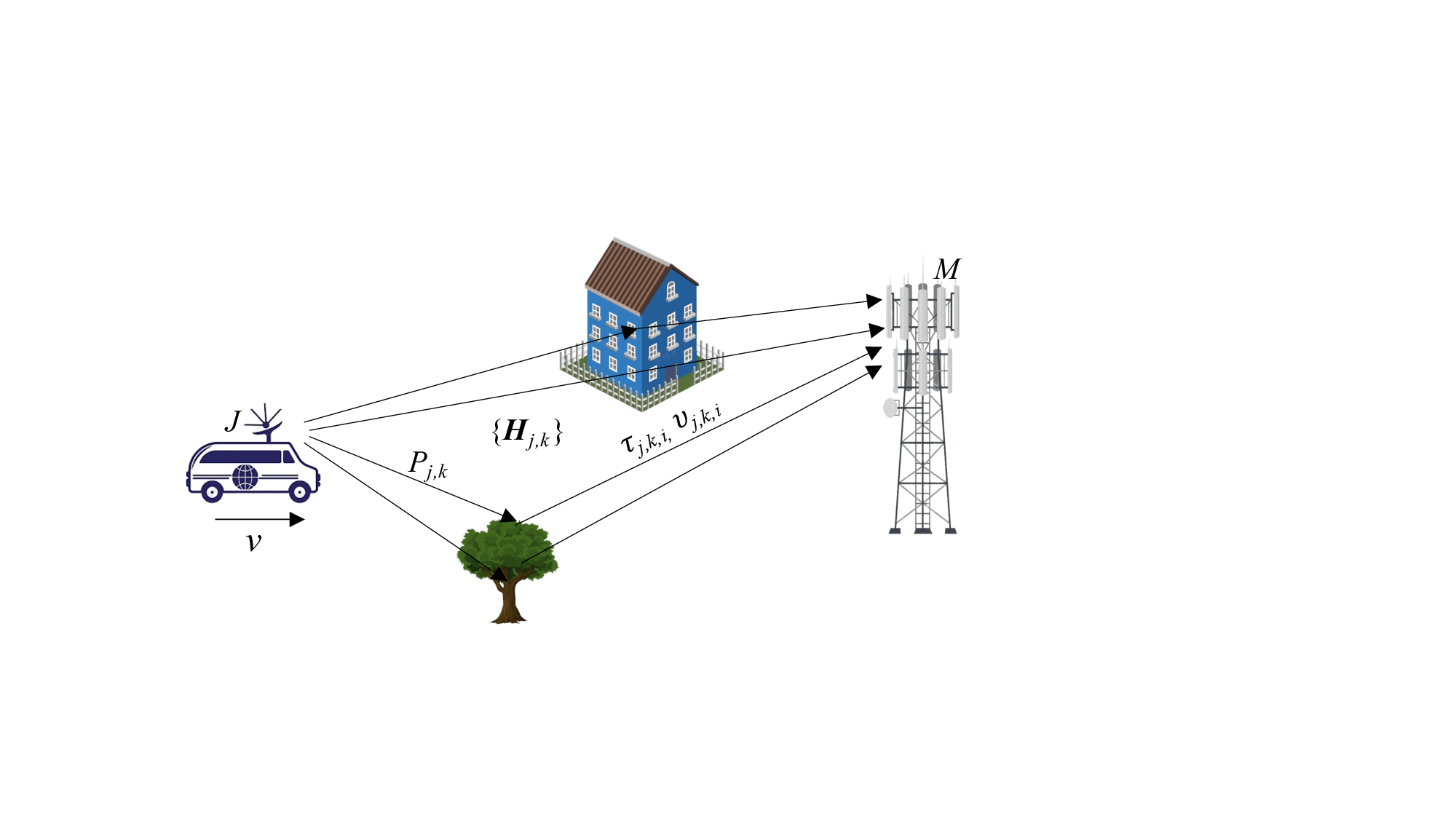
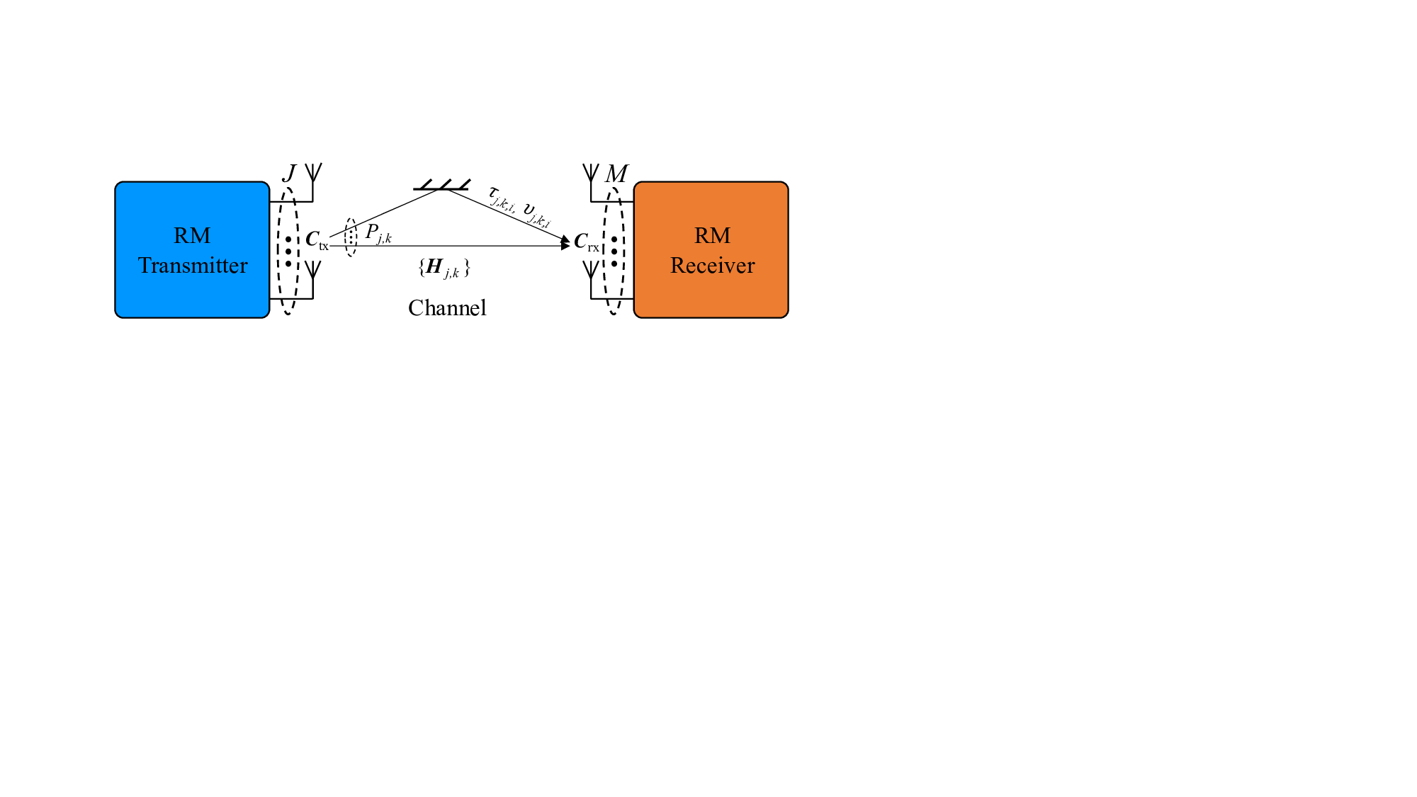
Note that the replica MAP BER and capacity optimality of RM rely on certain assumptions, such as large-scale systems and unique SE fixed points (Assumptions 1 and 2). When these conditions are not met, the combination of RM and CD-MAMP may experience performance degradation. For instance, the optimality and coding principles of CD-MAMP and CD-OAMP/VAMP may not hold in small-to mediumdimensional systems. A promising research avenue, inspired by [65], is to leverage AI techniques to facilitate the design of finite-length coding and detection algorithms. Meanwhile, under extremely harsh wireless channels, the equivalent channel matrices may still belong to the universality class U but with large condition numbers, causing severe instability-an open problem for message passing algorithms. Thus, integrating {H k,j } in MIMO RM systems with a mobile transmitter with J antennas and a receiver with K antennas, where P k,j denotes the maximal number of multipaths between the j-th transmit antenna and the k-th receive antenna, τ k,j,i channel delay and ν k,j,i Doppler shift in the i-th path, and Ctx and Crx correlation-shaping matrices at the transmitter and receiver, respectively, 1 ≤ i ≤ P k,j , 1 ≤ j ≤ J and 1 ≤ k ≤ K.

AI techniques holds promise for overcoming this bottleneck. In summary, RM offers a practical framework for optimal transceiver design, and its integration with AI is expected to enable broader applicability across diverse scenarios.

In this section, we provide numerical results to demonstrate the achievable rates and finite-length BER/BLER performance of the random multiplexing systems with CD-MAMP receiver, optimal power allocation, and channel coding.

Consider a time-varying multipath MIMO channel, as shown in Fig. 10,i

, and channel impulse response H k,j [u, ℓ] between jth transmit antenna and k-th receive antenna, 1 ≤ j ≤ J, 1 ≤ k ≤ K, is given by

H k,j,i e j2πν k,j,i (uTs-ℓTs) P rc (ℓT s -τ k,j,i ),

denotes the maximal number of channel taps, P k,j is the maximal number of multipaths, T s denotes the system sampling interval, H k,j,i , τ k,j,i , and ν k,j,i denote the channel gain, delay, and Doppler shift in the i-th path, respectively. P rc (•) is the overall raised-cosine rolloff filter when the practical root raised-cosine (RRC) pulse shaping filters are employed at the transceiver to control signal bandwidth and reject out-of-band emissions. Meanwhile, H k,j,i also contains the spatial correlations among the antennas [66, Equation ( 6)], i.e., H k,j,i = Hi [k, j], where

with IID complex Gaussian random matrix H i , correlationshaping matrices C rx and C H tx obtained by the Cholesky

where ρ tx , ρ rx ∈ [0, 1) denote the correlation level at R tx and R rx , respectively. Here, we assume that ρ tx = ρ rx = ρ.

We consider that the carrier frequency is 4 GHz with ∆f = 15 kHz, the velocity of the device is v ∈ {150, 300} km/h with a maximum Doppler frequency shift ν max ∈ {555.5, 1111} Hz, P k,j = 5, and the channel Doppler shift is generated by using Jakes information [62]. The RRC rolloff factor in the transceiver is set at 0.4. Here, SISO and MIMO random multiplexing systems are considered with (J, K) = (1, 1), (2, 2), (4,4), and (8,4), where ρ ∈ {0.3, 0.6} and M = N ∈ {2048, 1024, 512, 256}, respectively. In addition, the common QPSK, 8PSK, 16QAM, and Gaussian signaling are employed. Here, the random transform matrix is set as Ξ = ΠT HW for Figs. 11 and 12 and Ξ = ΠF H for Figs. 131415161718, where T HW denotes the normalized Hadamard-Walsh transform matrix and F H the normalized IDFT matrix.

Fig. 11 shows BER comparisons of MIMO systems with and without random multiplexing, where CD-OAMP/VAMP and CD-MAMP detectors are employed, (J, K) = (2, 2), M = N = 1024, and ρ = 0.3. As can be seen, thanks to the random multiplexing, both CD-MAMP and CD-OAMP/VAMP achieve the same BER performance consistent with the predictions of SE analysis in (24) and (26). In contrast, when no multiplexing is employed and the BER curves are at 10 -4 , the BER performance of CD-OAMP/VAMP deteriorates significantly by approximately 13 dB, while CD-MAMP converges to a BER of around 10 -2 . This indicates that channel matrices in practical communication systems rarely satisfy the input isotropy condition, resulting in degraded detection performance. Random multiplexing is therefore required to ensure that the equivalent channel matrix meets the input isotropy condition for CD-MAMP and CD-OAMP/VAMP detectors, enabling replica-MAP BER performance. These results are presented for the first time in this paper.

Fig. 12 illustrates the BER comparisons of random multiplexing, OFDM, OTFS, and AFDM in MIMO systems with CD-OAMP/VAMP and CD-MAMP detectors, where QPSK signaling is employed, (J, K) = (2, 2), and M = N = 1024. To be fair, we ensure that the multiplexing systems use the same bandwidth, i.e., the subcarrier spacing is ∆f kHz for OTFS, and ∆f Q kHz for IFDM, AFDM, and OFDM, where the OTFS multiplexing matrix is F H Q ⊗ I P with Q = 32 and P = 32. For BER curves of 10 -5 , it can be clearly seen that random multiplexing with CD-MAMP can achieve about a 11 dB gain with much lower complexity than OTFS/AFDM with CD-OAMP/VAMP, which also significantly outperforms OFDM with LMMSE. These results are similar to that reported in [52]. This also indicates that CD-OAMP/VAMP is no longer replica MAP optimal for existing OTFS and AFDM. The design of low-complexity, near-optimal detectors for OTFS and AFDM remains an open challenge.

Fig. 13 shows the BER comparisons of random multiplexing with optimal-MAP power allocation (PA) in (43), uniform PA, and channel parallelization via SVD with Gaussian and QPSK water filling, where QSPK signaling is employed. In random multiplexing, the optimal power allocation, aimed at achieving MAP performance, can achieve a 2 dB gain over uniform power allocation. In contrast, waterfilling for Gaussian and QPSK signals using channel parallelization via SVD decomposition results in a significant performance loss of more than 12 dB. This confirms the optimality of power allocation in random multiplexing.

Based on Theorem 3, we provide the achievable rate analysis of CD-MAMP in MIMO random multiplexing systems.

• Uniform Power Allocation: Fig. 14 shows the maximum achievable rates of CD-MAMP in MIMO random multiplexing systems with (J = 8, K = 4), ( M = N = 256), uniform power allocation, and {QSPK, 8PSK, 16QAM, Gaussian} signaling when CSI is unknown at the transmitter and available only at the receiver. Note that the achievable rate of CD-MAMP increases monotonically with the signal constellation order, where it converges to a constant value for discrete signaling and increases monotonically for Gaussian signaling as the SNR increases. Although Fig. 14 resembles our previous work [14], [15], the earlier study relied on the channel matrix being rightunitarily invariant, whereas this paper leverages random multiplexing to remove the need for such idealized channel assumptions. In contrast, a conventional cascading CD-MAMP (CAS-CD-MAMP) receiver is used as a baseline method, as defined in [67], [68], which operates by first using CD-MAMP for detection and then utilizing SE (ρ, p)dρ. Note that in this scenario, its achievable rate of CAS-CD-MAMP decreases instead with increasing signal constellation order.

• Optimal Power Allocation: Fig. 15 shows the achievable rate comparison of CD-MAMP with random multiplexing and channel parallelization via SVD in MIMO linear systems, where QPSK signaling is employed. When CSI is available in the transmitter, power allocation is employed to enhance the system capacity. For MIMO random multiplexing linear systems, the optimal power allocation in (45) has a 3 dB gain over the uniform power allocation at the same achievable rate and achieves the optimal rate for Gaussian signaling with Gaussian waterfilling in [20,Sec. 10.4] when SNR < 10 dB. Compared to conventional waterfilling for QPSK signaling based on channel parallelization, random multiplexing with optimal power allocation can achieve nearly a twofold rate improvement in the high SNR region (i.e., SNR > 10 dB). Fig. 16 shows the achievable rate comparison of CD-MAMP with random multiplexing and channel parallelization via SVD in MIMO linear systems, where 16QAM signaling is employed. Similar to the QPSK case, the random multiplexing with optimal power allocation can achieve the optimal rate for Gaussian signaling, a 3 dB gain over the random multiplexing with uniform power allocation for SNR ≤ 15 dB, and a 1.5 bits improvement per symbol for SNR > 15 dB. II and well-designed P2P irregular LDPC (Irre-LDPC) codes in [69] in MIMO random multiplexing systems, where (J, K) = (8, 4), M = N = 256, ρ = 0.6, P k,j = 5, and v = 300 km/h.

Fig. 17 shows the BLER comparisons of the different multiplexing with 5G-NR LDPC codes in MIMO linear systems, where the coding rate is 0.625 and coding length is 2048, (J, K) = (4, 4), M = N = 512, ρ = 0.6, P k,j = 5, v = 300 km/h. To be consistent with practical commercial communication systems, we employ CAS-MAMP for random multiplexing and CAS-OAMP/VAMP for OFDM, OTFS, and AFDM. Note that the gap between the BLER curve of random multiplexing with CAS-MAMP at 10 -4 and the corresponding performance limit is 2 dB, which achieves up to a 2 dB gain with lower complexity compared to OTFS, AFDM, and OFDM. This also validates the advantages of random multiplexing in 5G-NR LDPC coded linear systems. Fig. 18 provides the BER comparisons of the optimized irregular LDPC codes in Table II and well-designed SISO irregular LDPC codes in [69] for MIMO random multiplexing systems, where capacity-optimal power allocation (PA) in (45) and uniform PA are employed for QPSK signaling with M = N = 256, (J, K) = (8, 4), P k.j = 5, ρ = 0.6, and v = 300km/h. The degree distributions of P2P irregular LDPC codes are λ(X) = 0.24426x + 0.25907x 2 + 0.01054x 3 + 0.05510x 4 +0.01455 7 +0.01275x 9 +0.40373x 11 and µ(X) = 0.25475x 6 + 0.73438x 7 + 0.01087x 8 , whose rate R LDPC is 0.5 and the decoding threshold is 0.18 dB away from the P2P-AWGN capacity. Notably, with optimized and irregular LDPC codes, the capacity-optimal PA can achieve about 4.25 dB and 3 dB gains over the uniform PA, respectively. Furthermore, for fixed capacity-optimal and uniform PA, the optimized LDPC codes outperform the P2P irregular LDPC codes by about 5.95 dB and 4.7 dB gains. This indicates that the well-designed P2P irregular LDPC codes are not optimal anymore with significant performance losses in MIMO random multiplexing systems.

This paper presents a random multiplexing framework that decouples the multiplexing process from channel matrix dependencies, thereby enabling its application to arbitrary normbounded and spectrally convergent channel environments. By employing a random transformation, the random multiplexing builds an equivalent input-isotropic channel matrix in the random transform domain, facilitating the asymptotic replica MAP-BER optimality of AMP-type detectors. To further enhance efficiency, a CD-MAMP detector is considered, which effectively leverages the sparsity of time-domain channels and the input isotropy of the transform-domain channels, significantly reducing computational complexity without compromising detection performance. Furthermore, optimal power allocation strategies are developed to minimize the MAP BER and maximize the constrained channel capacity, complemented by the establishment of optimal coding principles and the constrained capacity optimality of CD-MAMP. The random multiplexing framework demonstrates remarkable versatility across diverse wireless applications, delivering advantages in spectral efficiency, and compatibility with established multiplexing techniques. Numerical results show that in correlated time-varying multipath MIMO channels, random multiplexing achieves BER and BLER performance improvements of up to 2 ∼ 10 dB compared to OFDM/OTFS/AFDM schemes, including conventional multiplexing and SISO channel coding, under both uniform and optimized power allocation, as well as with optimal channel coding strategies.

Future work will explore: 1) Robustness against burst noise in practical channels, leveraging random multiplexing’s ability to convert such noise into equivalent white Gaussian noise; 2) Enhanced physical layer security, where the random transform matrix acts as an encryption key to thwart eavesdroppers; and 3) Applications to sparse regression coded linear systems, extending the theoretical framework of compressed random multiplexing to systems with structured sparsity. These avenues will further validate the versatility and advantages of where 1 N denotes the N -dimensional all-ones vector, α and β are the averages of diagonal and off-diagonal entries of B respectively, i.e.,

Proof: See Appendix B-C. By Lemma 20, we have

where

From ( 71), we have

In addition,

From ( 77), ( 80), ( 83) and (84), we obtain that

for any fixed k ∈ N * , ϵ > 0. Finally, we take a union bound over k ∈ N * and ϵ ∈ Q + to finish the proof.

We first state the following lemma, a straightforward complex-valued extension of [71,Theorem 4.3].

Lemma 21. For any B ∈ C N ×N and t > 0, we have

where

where π :

Since

there exists explicit universal constants C such that

Let P be the permutation matrix corresponding to π, i.e.,

the entries of M can be expressed as

where u (i) is the i-th row of O and v (j) is the j-th column of QΛQ H P H O H , i.e.,

where e i denotes the i-th standard basis vector. Next, we apply the concentration inequality in (94) with s = 4 ln N to obtain

It can be verified that

Utilizing the inequalities:

we obtain

for any i, j ∈ [N ]. Finally, we take a union bound over i, j to finish the proof.

Let π : [N ] → [N ] be the permutation corresponding to P :

Hence, for any i, j ∈ [N ],

.

When i = j, the probability of π(i) = k is 1/N . As a result, Thus, we have completed the proof.

Our goal is to prove that [γ SE (v, p)] -1 = N N i=1 (v -1 + σ -2 σ 2 i p i ) -1 -1 (106) is concave w.r.t p. Since v > 0 and σ -2 σ 2 i ≥ 0, it follows from the concavity of

where pN = [p i , • • •, pN ] with pi ≡ v -1 + σ -2 σ 2 i p i > 0. We prove the concavity of g N ( pN ) by induction on N .

• When N = 1, g 1 (p 1 ) = p1 is concave.

• When N = 2, the Hessian matrix of g 2 (p 1 , p2 ) is

Since tr{H g2 } = -2(p 2 1 + p2 2 )/(p 1 + p2 ) 3 < 0 and det(H g2 ) = 0, the eigenvalues of H g2 must be one zero and one non-positive number. Thus, H g2 ⪯ 0, meaning that g 2 (p 1 , p2 ) is concave.

• When N ≥ 2, suppose that g N ( pN ) is concave. Then, for any 0 ≤ α ≤ 1, ᾱ = 1 -α, we have αg N +1 ( pN+1 ) + ᾱg N +1 (q N +1 ) = αg 2 g N ( pN ), pN+1 + ᾱg 2 g N (q N ), q N +1 (a)

≤ g 2 αg N ( pN ) + ᾱg N (q N ), αp N +1 + ᾱq N +1

Let z = v -1 and v = N ṽ. Therefore, [γ -1 SE (ṽ, p)] -1 can be formulated as

where g -1 (v, p) is the inverse function of g(z, p) w.r.t. z, given by v = g(z, p) = N i=1 (z + pi ) -1 .

(112)

It then suffices to prove the convexity of g -1 (v, p).

The following equation is obtained by taking the partial derivative of both sides of g -1 (v, p) -z = 0 w.r.t. pi , treating z as a variable independent of p.

i.e.,

The relationship between the first-order partial derivatives of an inverse function and its original function is given by the following equation: The second order partial derivatives are expressed as follows:

where

i , and (a) follows z = g -1 (v, p) and (117). Similarly, we have

The convexity of g -1 (v, p) can be established by proving that the Hessian matrix ∇ 2 p g -1 (v, p) is semi-positive definite. Given that Ω 2 = N i=1 a 2 i > 0, the task reduces to proving the semi-positive definiteness of Ω 3 2 2 ∇ 2 p g -1 (v, p), which can be shown by verifying the non-negativity of its quadratic form, i.e., ∀x ∈ R N ,

a 2 i a 2 j x i x j Ω 3 -(a

Thus, we have completed the proof.

Let H = U H Σ H V H H and P = U P Σ P V H P denote the singular value decomposition of H and P , respectively. The proof is completed by establishing the following two lemmas. Lemma 22. Choosing U P = V H with arbitrary unitary V P minimizes the MAP BER of the power-allocated system with random multiplexing in (28).

Proof: See Appendix E-A. Lemma 23. Choosing U P = V H with arbitrary unitary V P maximizes the constrained capacity of the power-allocated system with random multiplexing in (28).

Proof: See Appendix E-B.

We formulate the problem as P 3.0 : min (123c)

where γ(v ϕ t , Q) denotes the posterior variance w.r.t Q, and

As a result, Problem P 3 can be rewritten as

s.t. tr{Q} = P sum . (125b) Arbitrary V P is optimal since Q is independent to V P . Next, we introduce a crucial lemma proposed in [19].

Lemma 24 (Posterior Variance [19]). For v > 0,

where γ(•) is given in (123e), and Q diag denotes the diagonal of Q with zeros elsewhere.

Proof: Building on the proof in [19], we provide the omitted convexity proof of γ(v, Q) w.r.t Q. See Appendix E-C for details.

From Lemma 24 and the fact that tr{Q} = tr{Q diag }, it is clear that choosing U P = V H and arbitrary V P is optimal to minimize the MAP BER of the system in (28).

Following Q ≡ V H H P P H V H in (124), we formulate the problem as

where

where C MIMO (Q) is from [14, Theorem 1], γ(v, Q) is given in (123e). Arbitrary V P is optimal since Q is independent to V P . Next, we introduce an important lemma.

Lemma 25. For v > 0,

where γ-1 (v, Q) denotes the inverse function of γ(ṽ, Q) in (123e) w.r.t ṽ > 0.

Proof: For ṽ > 0, γ(ṽ, Q) is always positive and strictly increasing w.r.t ṽ, i.e., γ(ṽ 1 , Q) > γ(ṽ 2 , Q) > 0 if and only if ṽ1 > ṽ2 > 0. (130) Furthermore, following Lemma 24, we have γ(ṽ, Q diag ) ≤ γ(ṽ, Q).

(131) Thus, for any v > 0, γ(ṽ

which means that γ-1 (v, Q diag ) ≥ γ-1 (v, Q). Thus, we completed the proof. From Lemma 25 and (128), we have C MIMO (Q diag ) ≥ C MIMO (Q), where tr{Q} = tr{Q diag } always holds. Note that the entries in Q diag are the same as those in Σ 2 P . Thus, choosing U P = V H with V P arbitrary is optimal to maximize the constrained capacity of the system in (28).

Let g(v, Q) = tr v -1 I + σ -2 Σ H QΣ H H -1 . It is equivalent to prove that g(v, Q diag ) ≤ g(v, Q). First, we show the convexity of g(v, Q) w.r.t Q, which is omitted in [19].

Lemma 26 (convexity). For v > 0 and Hermitian positive semidefinite matirx Q,

is convex w.r.t Q.

Proof: Let B = v -1 I + σ -2 Σ H QΣ H H , which preserves convexity since it is an affine function of Q. Thus, we only need to show that tr{B -1 } is convex w.r.t Hermitian positive definite B. It is known that x -1 is a operator convex function w.r.t x ∈ (0, ∞) [72], i.e., for any Hermitian positive definite B 1 and B 2 , and α ∈ [0, 1],

Subsequently, we have

which implies that tr{B -1 } is convex w.r.t Hermitian positive definite B. Hence, we completed the proof.

Next, the proof is the same as that in [19]. Let J 1 , • • •, J T denotes all the possible M × M diagonal matrices with diagonal entries of 1 or -1, where T = 2 M . For 1 ≤ i ≤ T , it can be verified that g(v, Q) = g(v, J i QJ i ).

(136) Moreover, from [73], we have

Therefore,

≥ g v, 1 T T i=1

where (a) holds due to Lemma 26 and Jensen’s inequality. Hence, we have completed the proof.

are independent of x and s, with IID Gaussian columns and jointly Gaussian rows that satisfy w t ∼ CN (0, v ϕ t,t I) with E{w t (w t ′ ) H } = v ϕ t,t ′ I, and z t ∼ CN (0, v γ t,t I) with E{z t (z t ′ ) H } = v γ t,t ′ I. t×t remain invariant under the RT and IRT in

t ) is employed in the linear detector (LD) and the MMSE demodulator φt (s in t ) = E{s|s in t = s + v γ t z, s ∼ P s } is employed in the nonlinear detector

• , v ϕ * ), where v γ * = lim * ) as that of CD-OAMP/VAMP in (25).

s.t. tr{P PH } = P sum . (121b)Since the MAP demodulation function Q S (•) is monotonically decreasing, it is reduced toP 3 : max P ρ * (P ),(122a)s.t. tr{P P H } = P sum ,(122b)where ρ * t ] -1 I + σ -2 P H H H HP -1

s.t. tr{P PH } = P sum . (121b)Since the MAP demodulation function Q S (•) is monotonically decreasing, it is reduced toP 3 : max P ρ * (P ),(122a)s.t. tr{P P H } = P sum ,(122b)

s.t. tr{P PH } = P sum . (121b)Since the MAP demodulation function Q S (•) is monotonically decreasing, it is reduced toP 3 : max P ρ * (P ),(122a)s.t. tr{P P H } = P sum ,

s.t. tr{P PH } = P sum . (121b)Since the MAP demodulation function Q S (•) is monotonically decreasing, it is reduced toP 3 : max P ρ * (P ),(122a)

s.t. tr{P PH } = P sum . (121b)Since the MAP demodulation function Q S (•) is monotonically decreasing, it is reduced toP 3 : max P ρ * (P ),

s.t. tr{P PH } = P sum . (121b)Since the MAP demodulation function Q S (•) is monotonically decreasing, it is reduced to

s.t. tr{P PH } = P sum . (121b)

s.t. tr{P PH } = P sum . (121b

s.t. tr{P PH } = P sum . (

s.t. tr{P P

In this paper, OAMP and VAMP are collectively referred to as OAMP/VAMP due to their underlying equivalence.

Strictly speaking, if J is random but independent of D, and almost surely satisfies the conditions in items 2 and

3, then it follows that JD almost surely lies in U . For brevity, we do not distinguish this case from the deterministic one in this paper.

A RT matrix Ξ can be constructed as follows: First, randomly generate a normalized IID Gaussian matrix A. Then, conduct the SVD decomposition of A, i.e., A = U A Σ A V H A . Finally, set Ξ as V H A .