Causify DataFlow: A Framework For High-performance Machine Learning Stream Computing

The goal of DataFlow is to increase the productivity of data scientists by empowering them to design and deploy systems with minimal or no intervention from data engineers and devops support.

Guiding desiderata in the design of DataFlow include:

(1) Support rapid and flexible prototyping with the standard Python/Jupyter/data science tools (2) Process both batch and streaming data in exactly the same way (3) Avoid software rewrites in going from prototype to production (4) Make it easy to replay stream events in testing and debugging (5) Specify system parameters through config (6) Scale gracefully to large data sets and dense compute These design principles are embodied in the many design features of DataFlow, which include:

(1) Computation as a direct acyclic graph. DataFlow represents models as direct acyclic graphs (DAG), which is a natural form for dataflow and reactive models typically found in real-time systems. Procedural statements are also allowed inside nodes. (2) Time series processing. All DataFlow components (such as data store, compute engine, deployment) handle time series processing in a native way. Each time series can be univariate or multivariate (e.g., panel data) represented in a data frame format.

(3) Support for both batch and streaming modes. The framework allows running a model both in batch and streaming mode, without any change in the model representation.

The same compute graph can be executed feeding data in one shot or in chunks (as in historical/batch mode), or as data is generated (as in streaming mode). DataFlow guarantees that the model execution is the same independently on how data is fed, as long as the model is strictly causal. Testing frameworks are provided to compare batch/streaming results so that any causality issues may be detected early in the development process. (4) Precise handling of time. All components automatically track the knowledge time of when the data is available at both their input and output. This allows one to easily catch future peeking bugs, where a system is non-causal and uses data available in the future. (5) Observability and debuggability. Because of the ability to capture and replay the execution of any subset of nodes, it is possible to easily observe and debug the behavior of a complex system. (6) Tiling. DataFlow’s framework allows streaming data with different tiling styles (e.g., across time, across features, and both), to minimize the amount of working memory needed for a given computation, increasing the chances of caching computation. (7) Incremental computation and caching. Because the dependencies between nodes are explicitly tracked by DataFlow, only nodes that see a change of inputs or in the implementation code need to be recomputed, while the redundant computation can be automatically cached. (8) Maximum parallelism. Because the computation is expressed as a DAG, the DataFlow execution scheduler can extract the maximum amount of parallelism and execute multiple nodes in parallel in a distributed fashion, minimizing latency and maximizing throughput of a computation. (9) Automatic vectorization. DataFlow DAG nodes can apply a computation to a crosssection of features relying on numpy and Pandas vectorization. (10) Support for train/prediction mode. A DAG can be run in ‘fit’ mode to learn some parameters, which are stored by the relevant DAG nodes, and then run in ‘predict’ mode to use the learned parameters to make predictions. This mimics the Sklearn semantic.

There is no limitation to the number of evaluation phases that can be created (e.g., train, validation, prediction, save state, load state). Many different learning styles are supported from different types of runners (e.g., in-sample-only, in-sample vs out-of-sample, rolling learning, cross-validation). (11) Model serialization. A fit DAG can be serialized to disk and then materialized for prediction in production. (12) Configured through a hierarchical configuration. Each parameter in a DataFlow system is controlled by a corresponding value in a configuration. In other words, the config space is homeomorphic with the space of DataFlow systems: each config corresponds to a unique DataFlow system, and vice versa, each DataFlow sytem is completely represented by a Config. A configuration is represented as a nested dictionary following the same structure of the DAG to make it easy to navigate its structure. This makes it easy to create an ensemble of DAGs sweeping a multitude of parameters to explore the design space. (13) Deployment and monitoring. A DataFlow system can be deployed as a Docker container. Even the development system is run as a Docker container, supporting the development and testing of systems on both cloud (e.g., AWS) and local desktop. Airflow is used to schedule and monitor long-running DataFlow systems. (14) Python and Jupyter friendly. The framework is completely implemented in highperformance Python. It supports natively ‘asyncio’ to overlap computation and I/O. The Section 4.2). This design unifies batch and streaming execution semantics within a single framework, enabling models developed in batch mode to execute identically in streaming production environments without code modification.

1.2. Definition of stream computing. In the computer science literature, several terms (such as event/data stream processing, graph computing, dataflow computing, reactive computing) are used to describe what in this paper we refer succintly to as “stream computing”.

By stream processing we refer to a programming paradigm where streams of data (e.g., time series or dataframes) are the objects of computation. A series of operations (aka kernel functions) are applied to each element in the stream.

Stream computing represents a paradigm shift from traditional batch processing and imperative languages, emphasizing real-time data handling, adaptability, and parallel processing, making it highly effective for modern data-intensive applications.

1.3. Core principles of stream computing. The core principles of stream computing are:

(1) Node-based architecture. In stream and dataflow programming, the code is structured as a network of nodes. Each node represents a computational operation or a data processing function. Nodes are connected by edges that represent data streams. (2) Data-driven and reactive execution. Execution in dataflow languages is data-driven, meaning that a node will process data as soon as it becomes available. Unlike imperative languages where the order of operations is predefined, in dataflow languages, the flow of data determines the order of execution. (3) Automatic parallelism. The Dataflow programming paradigm naturally lends itself to parallel execution. Since nodes operate independently, they can process different data elements simultaneously, exploiting concurrent processing capabilities of modern hardware. (4) Continuous data streams. Streams represent a continuous flow of data rather than discrete batches. Nodes in the network continuously receive, process, and output data, making them ideal for real-time data processing. (5) State management. Nodes can be stateful or stateless. Stateful nodes retain information about previously processed data, enabling complex operations like windowing, aggregation, or pattern detection over time. (6) Compute intensity. Stream processing is characterized by a high number of arithmetic operations per I/O and memory reference (e.g., it can be 50:1), since the same kernel is applied to all records and a number of records can be processed simultaneously. Furthermore, data is produced once and read only a few times. (7) Dynamic adaptability. The dataflow model can dynamically adapt to changes in the data stream (like fluctuations in volume or velocity), ensuring efficient processing under varying conditions. (8) Scalability. The model scales well horizontally, meaning one can add more nodes (or resources) to handle increased data loads without major architectural changes. (9) Event-driven processing. Many dataflow languages support event-driven models where specific events in the data stream can trigger particular computational pathways or nodes.

1.4. Applications of stream computing. Stream computing is a natural solution in a wide range of industries and scenarios. Table 1 presents representative application domains and their corresponding use cases.

DataFlow is a computational framework designed to build, test, and deploy artificial intelligence and machine learning models for unbounded tabular time series data. The framework addresses the unique challenges of processing streaming data where temporal ordering, causality, and reproducibility are essential requirements. DataFlow is particularly suited to domains including financial markets, IoT sensor networks, supply chain monitoring, and real-time analytics systems where time dependencies constitute a fundamental aspect of the modeling problem.

Core Abstractions. The central data model in DataFlow is the stream dataframe, a timeindexed tabular structure with a potentially unbounded number of rows. Unlike traditional batchoriented dataframes, stream dataframes model data as continuous sequences that arrive incrementally over time, reflecting the reality of production systems where data generation is ongoing and termination is not inherent to the process.

Computation in DataFlow is organized as a directed acyclic graph (DAG) of computational nodes. Each node receives a fixed number (possibly zero) of stream dataframes as input and produces a fixed number of stream dataframes as output. Nodes encapsulate transformations ranging from simple arithmetic operations to complex machine learning models. The DAG structure makes data dependencies explicit and enables the framework to exploit parallelism and perform incremental computation.

Tiling and Point-in-Time Idempotency. A distinguishing principle of DataFlow is the requirement that computations be tilable-that is, their correctness must not depend on how input data is partitioned along temporal or feature dimensions. Formally, a computation is tilable if it can operate on contiguous windows (tiles) of the input stream and produce outputs that are invariant to the tile boundaries, provided that each tile contains sufficient temporal context. This invariance is enforced through point-in-time idempotency: for any time point t, the output at t depends only on a fixed-length temporal window preceding t, known as the context window. Once a tile includes at least this context window length of historical data, the computed output at the tile’s right endpoint is guaranteed to match the output that would be obtained from processing the entire historical stream up to that point.

Point-in-time idempotency provides a formal correctness criterion that unifies batch and streaming execution. A model developed and validated on historical data in batch mode can be deployed in streaming mode with the assurance that, as long as causality is preserved, the outputs will be identical to those produced in batch evaluation. This property is enforced by the framework and can be automatically validated through tiling tests that partition data in multiple ways and verify output consistency.

The tiling principle and point-in-time idempotency requirement enable several critical capabilities:

(1) Unified batch and streaming execution. The same model specification executes identically in batch mode (processing historical data in large chunks) and streaming mode (processing data as it arrives), eliminating the need for separate implementations and reducing development-production discrepancies. (2) Causality enforcement. Because outputs at time t depend only on data from times s ≤ t, the framework prevents future-peeking errors that commonly arise in batch-oriented development. Violations of causality manifest as tile-dependent outputs and are automatically detectable through tiling validation tests. (3) Memory-bounded computation. Tiles may be sized to fit within available memory resources while maintaining correctness, enabling processing of arbitrarily large historical datasets without requiring full in-memory representation.

(4) Replay and debugging. Real-time execution can be captured and replayed deterministically in development environments. The framework records input streams with precise knowledge timestamps, enabling systematic debugging of production failures by replaying exact sequences of events. (5) Parallelism and incremental computation. The DAG structure makes data dependencies explicit. Nodes with no dependency relationship may execute in parallel, and nodes whose inputs and implementations have not changed may skip recomputation by retrieving cached results. The framework automatically exploits these opportunities for optimization. (6) Vectorization across features. Stream dataframes support multi-level column indexing, enabling computations to be expressed in vectorized form across assets or features. This design leverages the computational efficiency of array-oriented libraries (e.g., NumPy, pandas) while maintaining compatibility with streaming semantics. ( 7) Model lifecycle management. Nodes may be stateful, supporting distinct fit and predict phases analogous to scikit-learn conventions. Trained models may be serialized and deployed to production environments with assurance that evaluation semantics remain consistent between research and deployment.

A tile is a contiguous temporal window of a stream dataframe whose length equals or exceeds the node’s context window requirement. For a node with context window length L, any tile of length τ ≥ L ending at time t contains sufficient information to compute the correct output at time t. The context window of a DAG is determined by the context windows of its constituent nodes and the dependencies encoded in the graph structure; the maximal context window over all source-to-sink paths defines the DAG-level context window.

An important consequence of point-in-time idempotency is that two tiles suffice for correct minibatch execution: providing two consecutive tiles of input data, each of length τ , ensures that all outputs in the second tile are computed correctly, even for time points near the tile boundary where the context window spans both tiles. This property (formalized in Theorem 4.24) underpins DataFlow’s ability to process historical data efficiently in batch mode while guaranteeing identical results to streaming execution.

The framework’s tile-based execution model, combined with explicit dependency tracking and causality enforcement, addresses the fundamental tension between the finite-data assumptions prevalent in data science tooling and the unbounded-data reality of production systems. By treating data as unbounded streams from the outset and imposing strict correctness criteria, DataFlow enables models to be developed, validated, and deployed within a unified computational model.

Conducting machine learning on streaming time series data introduces additional challenges beyond those encountered with machine learning on static data. These challenges include overfitting, feature engineering, model evaluation, data pipeline engineering. These issues are compounded by the dynamic nature of streaming data.

In the following we list several problems in time-series machine learning and how DataFlow solves these problems.

3.1. Prototype vs Production. Data scientists typically operate under the assumption that all data is readily available in a well-organized data frame format. Consequently, they often develop a prototype based on assumptions about the temporal alignment of the data. This prototype is then transformed into a production system by rewriting the model in a more sophisticated and precise framework. This process may involve using different programming languages or even having different teams handle the translation. However, this approach can lead to significant issues:

• Converting the prototype in production requires time and effort • The translation process may reveal bugs in the prototype.

• Assumptions made during the prototype phase might not align with real-world conditions.

• Discrepancies between the two model can result in additional work to implement and maintain two separate models for comparison. DataFlow addresses this issue by modeling systems as directed acyclic graphs (DAGs), which naturally align with the dataflow and reactive models commonly used in real-time systems. Each node within the graph consists of procedural statements, similar to how a data scientist would design a non-streaming system.

DataFlow enables the execution of a model in both batch and streaming modes without requiring any modifications to the model code. In batch Mode, the graph can be executed by processing data all at once or in segments, suitable for historical or batch processing. In streaming mode, the graph can also be executed as data is presented to the model, supporting real-time data processing.

Frequency of Model Operation. The required frequency of a model’s operation often becomes clear only after deployment. Adjustments may be necessary to balance time and memory requirements with latency and throughput, which require changing the production system implementation, with further waste of engineering effort.

DataFlow enables the same model description to operate at various frequencies by simply adjusting the size of the computation tile. This flexibility eliminates the need for any model modifications and allows models to be always run at the optimal frequency requested by the application.

Non-stationarity time series. While the assumption of stationarity is useful, it typically only strictly holds in theoretical fields such as physics and mathematics. In practical, real-world applications, this assumption is rarely valid. Data scientists often refer to data drift as an anomaly to explain poor performance on out-of-sample data. However, in reality, data drift is the standard rather than the exception.

All DataFlow components, including the data store, compute engine, and deployment, are designed to natively handle time series processing. Each time series can be either univariate or multivariate (such as panel data) and is represented in a data frame format. DataFlow addresses non-stationarity by enabling models to learn and predict continuously over time. This is achieved using a specified look-back period or a weighting scheme for samples. These parameters are treated as hyperparameters of the system, which can be tuned like any other hyperparameters.

3.4. Non-causal Bugs. A common and challenging problem occurs when data scientists make incorrect assumptions about data timestamps. This issue is often called “future peeking” because the model inadvertently uses future information. A model is developed, validated, and fine-tuned based on these incorrect assumptions, which are only identified as errors after the system is deployed in production. This happens because the data scientist lacks an early, independent evaluation to identify the presence of non-causality.

Figure 1 illustrates a concrete example of this bug pattern. DataFlow offers precise time management. Each component automatically monitors the time at which data becomes available at both its input and output. This feature helps in easily identifying future peeking bugs, where a system improperly uses data from the future, violating causality. DataFlow ensures consistent model execution regardless of how data is fed, provided the model adheres to strict causality. Testing frameworks are available to compare batch and streaming results, enabling early detection of any causality issues during the development process.

3.5. Accurate Historical Simulation. Implementing an accurate simulation of a system that processes time-series data to evaluate its performance can be quite challenging. Ideally, the simulation should replicate the exact setup that the system will use in production. For example, to compute the profit-and-loss curve of a trading model based on historical data, trades should be computed using only the information available at those moments and should be simulated at the precise times they would have occurred. However, data scientists often create their own simplified simulation frameworks alongside their prototypes. The various learning, validation, and testing styles (such as in-sample-only and crossvalidation) combined with walkthrough simulations (like rolling window and expanding window) result in a complex matrix of functionalities that need to be implemented, unit tested, and maintained.

DataFlow integrates these components once and for all into the framework, to streamline the process and allow to running detailed simulation in the design phase. DataFlow supports many different learning styles from different types of runners (e.g., in-sample-only, in-sample vs out-ofsample, rolling learning, cross-validation) together with 3.6. Debugging production systems. The importance of comparing production systems with simulations is highlighted by the following typical activities:

• Quality Assessment: To evaluate the assumptions made during the design phase, ensuring that models perform consistently with both real-time and historical data. This process is often called “reconciliation between research and production models.” • Model Evaluation: To assess how models respond to changes in real-world conditions.

For example, understanding the impact of data arriving one second later than expected.

• Debugging: Production systems occasionally fail and require offline debugging. To troubleshoot production models by extracting values at internal nodes to identify and resolve failures.

In many engineering setups, there is no systematic approach to conducting these analyses. As a result, data scientists and engineers often rely on cumbersome and time-consuming ad-hoc methods to compare models.

DataFlow solves the problem of observability and debuggability of models by easily allowing to capture and replay the execution of any subset of nodes. In this way, it is possible to easily observe and debug the behavior of a complex system. This comes naturally from the fact that research and production systems are the same, from the accurate timing semantic of the simulation kernel. • During the research phase, data scientists perform numerous simulations to explore the parameter space. It is crucial to systematically specify and track these parameter sweeps • Once the model is finalized, the model parameters must be fixed and these parameters should be deployed alongside the production system In a DataFlow system it is easy to generate variations of DAGs using a declarative approach to facilitate the adjustment of multiple parameters to comprehensively explore the design space.

• Each parameter is governed by a specific value within a configuration. This implies that the configuration space is equivalent to the space of DataFlow systems: each configuration uniquely defines a DataFlow system, and each DataFlow system is completely described by a configuration • A configuration is organized as a nested dictionary, reflecting the structure of the Directed Acyclic Graph (DAG). This organization enables straightforward navigation through its structure 3.9. Challenges in time series MLOps. The complexity of Machine Learning Operations (MLOps) arises from managing the full lifecycle of ML models in production. This includes not just training and evaluation, but also deployment, monitoring, and governance. DataFlow provides solutions to MLOps challenges fully integrated in the framework. In mathematical terms, a dataframe can be described as a two-dimensional (or more, as described below) labeled data structure, similar to an array but with more flexible features.

A dataframe df can be represented as:

where:

• m is the number of rows (observations).

• n is the number of columns (variables).

• a ij represents the element of the Dataframe in the i-th row and j-th column.

Remark 4.4. Some characteristics of dataframes are:

(1) Labeled axes:

• Rows and columns are labeled, typically with strings, but labels can be of any hashable type. • Rows are often referred to as indices and columns as column headers.

(2) Heterogeneous data types:

• Each column j can have a distinct data type, denoted as dtype j • Common data types include integers, floats, strings, and datetime objects. (3) Mutable size:

• Rows and columns can be added or removed, meaning that the size of df is mutable.

• This adds to the flexibility as compared to fixed-size arrays. (4) Alignment and operations:

• Dataframes support alignment and arithmetic operations along rows and columns.

• Operations are often element-wise but can be customized with aggregation functions. (5) Missing data handling:

• Dataframes can represent missing data through NaN and N one objects.

• Dataframes provide tools to handle, impute, or remove missing data.

(6) Multidimensionality:

• Tensor-like objects are supported through row or column “multi-indices”.

• If time is the primary key, then multi-index columns can be used to support panel or higher-dimensional data at each timestamp.

Definition 4.5 (DataFlow data format). As explained in XYZ, raw data from DataPull is stored in a “long format”, where the data is conditioned on the asset (e.g., full_symbol). DataFlow transforms this into a multi-index wide format where the index is a timestamp, the outermost column index is the feature, and the innermost column index is the asset.

Long The transformation is accomplished using pandas pivot operations: The reason for this convention is that typically features are computed in a uni-variate fashion (e.g., asset by asset), and DataFlow can vectorize computation over the assets by expressing operations in terms of the features. E.g., we can express a feature as

Definition 4.6 (Stream dataframe). Intuitively, a stream dataframe is a time-indexed sequence of rows that may be arbitrarily long in the past and is typically extended online as new rows arrive, i.e., a dataframe with a potentially unbounded number of rows.

Let R denote the set of possible dataframe rows (records). A stream dataframe is a partial function X :

where T ≤tmax = {t ∈ T : t ≤ t max } for some t max ∈ T. The value t max is the current time of the stream dataframe.

We may represent a stream dataframe up to time t 0 visually as in Table 2.

Definition 4.7 (Computational Node). A computational node N with m inputs and n outputs is specified by a family of functions

Given m input stream dataframes X (1) , . . . , X (m) whose domains contain [s, t], the node produces n output stream dataframes

The number of inputs m and outputs n is node-specific; either may be zero.

As in the general paradigm of dataflow computing, DataFlow represents computation as a directed graph. Nodes represent computation and edges the flow of data from one computational node to another. In DataFlow, each node accepts one or more (fixed number of) tables as input and emits one or more (fixed number of) tables as output. Nodes may either be stateless or stateful. A computational node receives as input a (per-node) predefined number (which may be zero) of stream dataframes and emits as output a predefined number of stream dataframes. The number of outputs may be zero and may differ from the number of inputs.

A computation node has:

• a fixed number of inputs • a fixed number of outputs • a unique node id (aka nid)

• a (optional) state

Inputs and outputs to a computational nodes are tables, represented in the current implementation as Pandas dataframes. A node uses the inputs to compute the output (e.g., using Pandas and Sklearn libraries). A node can execute in multiple “phases”, referred to through the corresponding methods called on the DAG (e.g., fit, predict, save_state, load_state).

A node stores an output value for each output and method name. Further examples include nodes that maintain relevant trading state, or that interact with an external environment:

• Updating and processing current positions • Performing portfolio optimization

• Generating trading orders • Submitting orders to an API Definition 4.9 (Causal Computation). A distinguishing feature of DataFlow is how time series are handled. Within each node, computation must be causal.

To introduce this notion, we consider the case where the (row) index of the tabular data is a time-based index. For convenience, we assume that the index is sorted according to the natural time ordering. We note that while data usually has multiple timestamps associated with it (e.g., event time, timestamps for various stages of processing, a final “knowledge timestamp” for the system), for the purposes of DataFlow, a single notion of time is chosen as primary key.

Definition 4.10 (Knowledge Time). Next, we posit the existence of a “simulation clock”, against which the data timestamps may be compared. In the case of real-time processing, the simulation clock will coincide with the system clock. In the case of simulation, the simulation clock is entirely independent of the system clock. In DataFlow, the simulation clock has initial and terminal times (except in real-time processing, where there is no terminal time) and advances according to a schedule. If, at any point in simulation time, a DataFlow node computation only depends upon data with timestamps earlier than the simulation time, then the computation is said to be causal. Remark 4.11 (Non-causal computations). Of course, any real-time system must be causal (any computation it performs necessarily only utilizes data available to it at the time of the computation). In many applications, the correctness of a computation performed at a certain point in simulation time is dependent upon having the complete set of data up to that point. While DataFlow relegates that function to DataPull in the case of real-time pipelines, violations of causal computation, either through human error or through data delays, are detectable in DataFlow through its testing and replay framework.

Note that there are some time series processing methods that prima facie are not causal. An example of this is fixed-interval Kalman smoothing, which, to calculate the smoothed data point at a particular point in time, requires data from the adjacent future time interval of fixed length. Provided the dependence upon future data is bounded in time, such techniques may be included in a causal framework through the proper choice of primary key timestamp. In the case of Kalman smoothing, this choice of timestamp would have the apparent effect of yielding smoothed data points with a delay equal to the fixed-interval of time required for the smoothing. Definition 4.12 (Incremental Computation). While latency-sensitive real-time systems are expected to perform computation incrementally, i.e., with every data update, an important observation to make is that, in many cases, causal computation need not be performed incrementally. For example, calculating point-to-point percentage change in a time series (such as calculating returns from prices) is causal, but may be vectorized over a batch. In practice, this means that simulation or batch computation need not be executed in the same way that a real-time system is.

where:

• each vertex v ∈ V is a computational node,

• each edge e = (u, v) ∈ E connects an output stream of u to an input stream of v.

A subset of incoming edges to G is designated as graph inputs, and a subset of outgoing edges as graph outputs.

Nodes are organized by the user into a directed acyclic graph (DAG).

Definition 4.14 (DataFlow DAG). A DataFlow DAG is a directed acyclic graph G = (V, E) where:

• each edge e = (u, v) ∈ E connects an output stream of u to an input stream of v. A subset of incoming edges to G is designated as graph inputs, and a subset of outgoing edges as graph outputs.

Nodes are organized by the user into a directed acyclic graph (DAG). (1) We say that L is a context window length for N if the following holds: for all t ∈ T and all intervals [s

for all input stream dataframes X (1) , . . . , X (m) we have (Y

(1) , . . . , Y

(2) , . . . , Y

(

(2) (t) for all j ∈ {1, . . . , n}. (2) If such an L exists, we say that N is point-in-time idempotent. The minimal such L (if it exists) is called the minimal context window length of N and denoted L N .

Intuitively, once the incoming window is at least L steps long, the latest-in-time output at t is independent of how far back in time the window starts. This is exactly the informal notion of point-in-time idempotency.

Figure 3 illustrates this concept with a concrete example using a moving average with context window L = 3. Remark 4.16 (Tilability as a computational property). Point-in-time idempotency is closely related to the property of tilability: a computation is tilable if its output does not depend on how input data is partitioned along the temporal axis, provided sufficient historical context is maintained. More precisely, for tiles

where L is the context window length and the restriction to output intervals ensures we only compare outputs that have sufficient context. Point-in-time idempotency guarantees that this equality holds at each time point independently, which in turn ensures tilability. This property enables a node to process data in arbitrary temporal chunks while producing consistent results, a fundamental requirement for unified batch-streaming execution. Another notable time series element of the DataFlow approach to computation is the notion of a lookback period. If computation at a certain point in simulation time, say t 1 , does not require timestamped data with timestamps earlier than t 0 < t 1 , then the lookback period at time t 1 is t 1 -t 0 > 0. In many cases, this lookback period is independent of the time t 1 , in which case we may refer to the quantity as the lookback period. More generally, we define the lookback period to be the supremum of lookback periods over all times t 1 . The lookback period places an effective lower bound on the amount of data required by a node to ensure computational correctness and has implications for how a DataFlow graph may be executed. Certain operations, e.g., exponentially weighted moving averages, have an effectively infinite lookback period. Through careful state management and bookkeeping, such operations may also be handled in DataFlow. Lemma 4.17 (Local dependence on trailing window). Let N be a point-in-time idempotent node with context window length L. Then for each output index j ∈ {1, . . . , n} there exists a function

such that for any time t ∈ T and any interval [s, t] with t -s + 1 ≥ L, if applying N on [s, t] yields outputs (Y (1) , . . . , Y (n) ), then Y (j) (t) = g j (X (1) (t -L + 1), . . . , X (1) (t)), . . . , (X (m) (t -L + 1), . . . , X (m) (t)) .

Proof. Fix j. For any tuple (r

L ), . . . , (r (1) , . . . , X (m) ) and set

L ), . . . , (r

We must show g j is well-defined. Consider any other choice of interval [s ′ , t ′ ] with t ′ -s ′ + 1 = L and streams X ′(i) that encode the same L-tuples. Extend the original and alternative intervals arbitrarily backwards to [s ′′ , t] and [s ′′′ , t ′ ], with s ′′ ≤ s and s ′′′ ≤ s ′ , and extend the streams accordingly. By point-in-time idempotency with window L, the output at time t (resp. t ′ ) is invariant under the choice of how far back the window starts, provided its length is at least L. Thus every such construction yields the same Y (j) (t), so g j is well-defined. Now take arbitrary input streams X (1) , . . . , X (m) and an interval [s, t] with t -s + 1 ≥ L. Let

and construct streams as above on an interval of length L ending at t. Point-in-time idempotency implies that Y (j) (t) is the same as if we had started the window at t -L + 1, hence it equals g j applied to the trailing L tuples, as claimed. □ Lemma 4.17 formalizes the intuitive claim that, once the context window is “filled,” the output at time t depends only on the last L time points of each input. .

The operation F (X) = X + X has context window L = 1 (no memory). Processing the full stream X 1 ∪ X 2 yields the same result as processing each tile independently and concatenating:

Example 2: Operations with memory. Consider a differencing operation F (X) t = X t -X t-1 , which has context window L = 2. To correctly process tile X 2 starting at t 3 , we must include the final observation from the previous tile: .

Applying F to the extended tile X2 and restricting output to [t 3 , t 4 ] produces the same result as if the entire stream had been processed at once. This requirement-extending tiles with sufficient context-is central to DataFlow’s tiling mechanism. More generally, operations with finite memory (such as rolling averages, exponential moving averages with recursive formulations, or FIR filters) can be made tilable by ensuring that each tile includes at least L preceding observations, where L is the node’s context window. 4.3. Stream dataframes and tiles. We now formalize tiles, which are contiguous windows of the stream dataframe that are at least as long as the context window. Definition 4.19 (Tile). Let X be a stream dataframe and let L ∈ N. A tile of length τ ∈ N ending at time t is the restriction X| [t-τ +1,t] for some τ ≥ L. The interval [t -τ + 1, t] is the temporal extent of the tile and t its right endpoint.

In Table 3 we depict a stream dataframe tile of length 4 ending at time point t 0 , with context window of length 3. We use blue text coloring to indicate the indices of inputs that are included in the context window (i.e., the last L = 3 points). Definition 4.20 (Ideal pointwise semantics). Let N be a point-in-time idempotent node with context window length L, and let X (1) , . . . , X (m) be input streams. For any t ∈ T and any s ≤ t with t -s

[s,t] (t) is independent of s, as long as t -s + 1 ≥ L. We define the ideal output of N at time t by

We now show that any tile whose length is at least the context window length produces the correct (ideal) output at its right endpoint.

Theorem 4.21 (Single-step tile correctness (streaming mode)). Let N be a point-in-time idempotent node with context window length L. Fix any tile length τ ≥ L, and let X (1) , . . . , X (m) be input streams. For a time t such that [t -τ + 1, t] is contained in the domain of each input, define

i.e., the output at the right endpoint t computed from the tile coincides with the ideal node output at t. Proof. By definition of the ideal semantics, for any s ≤ t -L + 1 we have

Point-in-time idempotency therefore guarantees correctness of the t 0 output for any tile of length at least the context window (e.g., length 3 or 4 in Table 3). We illustrate this in Table 4, where the text in blue indicates the context window inputs, and the text in orange indicates the corresponding point-in-time idempotent output.

When operating in streaming mode, the context window “slides” as time advances. In Table 5, we show how the context window advances as the next time point t 1 arrives, producing a new point-in-time idempotent output at t 1 . Let N be a node, τ ∈ N a tile length, and X (1) , . . . , X (m) input streams. For a time t such that I

and call the collection Y (j)

the mini-batch output tile corresponding to the second tile.

Theorem 4.24 (Two tiles suffice for tile-level idempotency). Let N be a point-in-time idempotent node with context window length L, and let τ ≥ L. Let X (1) , . . . , X (m) be input streams defined on a prefix T ≤tmax , and fix t ≤ t max such that [t -2τ + 1, t] ⊆ T ≤tmax . Then for every u ∈ [t -τ + 1, t] and every j ∈ {1, . . . , n}, Y

i.e., the mini-batch output tile over the second tile coincides with the ideal pointwise outputs. Moreover, these outputs are invariant under extending the input window further into the past.

Proof. Fix u ∈ [t -τ + 1, t] and j. By Lemma 4.17, there exists a function g j such that the value of the j-th output at time u depends only on the restriction of the inputs to

We first check J u ⊆ I

(2)

t . The right endpoint satisfies u ≤ t by assumption. For the left endpoint, we use u ≥ t -τ + 1 and L ≤ τ :

Consequently, when we apply N to I (u) is determined entirely by the inputs on J u and therefore coincides with the value obtained by applying N to any interval ending at u and containing J u with length at least L. By the definition of the ideal semantics, this value is exactly Y (j) (u). This proves the first part.

For invariance under further extension, consider any s ′ ≤ t -2τ + 1 and the extended window [s ′ , t]. The interval J u remains contained in [s ′ , t], and point-in-time idempotency with window L ensures that any earlier history prior to u -L + 1 does not affect the output at u. Hence the value at u computed from [s ′ , t] equals that computed from I (2) t , establishing the desired invariance. □ Theorem 4.24 justifies the mini-batch schematic shown in Figure 4 and Table 6. In Figure 4 and Table 6, we use purple (violet) to indicate the input context required for tile-level idempotency, and red to indicate the idempotent outputs associated with the tile-level context. Table 6. Temporal mini-batch processing

Note that outputs t -2 and t -3 in Table 6 have context windows spanning both tiles, as predicted by the proof of Theorem 4.24.

Remark 4.25 (Detecting incorrect tiled computations). The tilability property provides a practical method for validating the correctness of DataFlow implementations. Given a node (or DAG) purported to have context window length L, one may perform the following validation:

(1) Execute the node on the full historical stream to obtain reference outputs Y ref .

(2) Partition the same historical data into tiles of varying lengths τ 1 , τ 2 , • • • ≥ L with different temporal boundaries.

(3) Execute the node on each tiled partition (using two-tile windows as per Theorem 4.24) to obtain outputs Y (τ 1 ) , Y (τ 2 ) , . . . (4) Verify that Y (τ k ) = Y ref for all k up to numerical precision. Discrepancies between tiled and untiled outputs indicate one of three failure modes: (1) the stated context window L is insufficient; (2) the node implementation inadvertently accesses future data (violates causality); or (3) the node exhibits nondeterministic behavior or untracked dependencies.

This validation protocol is particularly valuable for detecting future-peeking bugs, where a computation inadvertently uses information from time t ′ > t when producing output at time t. Such errors are notoriously difficult to detect in batch-mode development but manifest immediately as tiling inconsistencies. DataFlow’s testing framework automates this validation, enabling early detection of causality violations during the development cycle.

Remark 4.26 (Tile size vs. DAG context window). Tile size τ is a user-selected parameter whose optimal value depends on use case, data requirements, and computational resources. For example, backtesting on a single machine may suggest a tile size dictated by memory constraints, while a near real-time system whose input frequency exceeds the decision-making frequency may suggest a small tile size. Latency-critical real-time applications suggest the minimum tile size, i.e., the DAG-level context window length. Crucially, τ is tunable and separate from the computational logic: the same DataFlow DAG may be used for both latency-critical real-time applications and large-scale historical backtests, with correctness guaranteed whenever τ is chosen to be at least the DAG context window. 4.5. Columnar grouping. Up to this point we have discussed tiling purely in terms of time indexing. DataFlow also supports columnar tiling, which allows the separation of computationally independent columns into separate tiles. This form of independence is easiest to interpret when operating with tiles with multilevel column indexing.

Formally, let U denote a finite index set of entities (e.g., customers), and let F denote a finite index set of features (e.g., “time spent”, “dollars spent”). The set of columns is then the Cartesian product C := U × F, and a stream dataframe row at time t may be written as

A columnar grouping is a partition

where each C k ⊆ C is a group of columns that we may tile and process jointly.

For example, suppose there is a column index level called “customer”, and to each customer there are associated fields “time spent” and “dollars spent”. We depict such a streaming dataframe in Table 7.

In this example, U = {A, B} and F = {time, $}, so C = {(A, time), (A, $), (B, time), (B, $)}. Table 7 depicts the restriction of the stream dataframe to these columns over time.

Suppose that one wishes to aggregate over a sliding time window the “time spent” column across all users, and that, separately, one wishes to identify the user who spends the greatest dollar amount in a given time window. In this contrived example, the “time” and “dollar” computations are independent, which allows one to tile according to column group (in addition to time).

Formally, let U = {A, B, . . . } and define feature-specific column groups

Let [t -3, t 0 ] be a time interval of length 4. Consider two functionals:

and a combining map Φ :

[s,t] (X| [s,t]×C 1 ), . . . , F

In this terminology, the “time spent” aggregation and “dollars spent” argmax are columnseparable with respect to P = {C time , C $ }, with K = 2 and two independent subcomputations F (1) and F (2) . Proof. This is immediate from the definition of column-separability: by assumption, for all X,

and each argument of Φ depends only on the restriction of X to the corresponding group C k . Thus the K subcomputations can be carried out independently and in parallel on the respective column-restricted tiles. □ Remark 4.30 (Cross-sectional tiling and computational independence). Proposition 4.29 establishes that computations may be partitioned not only along the temporal axis (as in temporal tiling) but also along the feature/entity axis when column-separability holds. This enables cross-sectional tiling, where the dataframe is partitioned into column-disjoint subsets that may be processed independently.

Cross-sectional tiling provides several benefits:

• Horizontal scalability. When processing thousands of entities (e.g., financial instruments, customers, sensors), column groups may be distributed across multiple machines, enabling data-parallel execution that scales linearly with the number of entities. • Memory efficiency. Large dataframes with many columns may exceed available memory.

Column-restricted tiles allow processing subsets that fit in memory, with results combined via the map Φ. • Heterogeneous processing. Different column groups may be assigned to processors with different characteristics (e.g., CPU vs. GPU) based on their computational requirements. Importantly, temporal and cross-sectional tiling may be composed : a dataframe may be partitioned along both time and column dimensions simultaneously, yielding a two-dimensional tiling that exploits independence along both axes. The resulting tiles are characterized by a time interval [s, t] and a column group C k , and correctness follows from the conjunction of temporal point-in-time idempotency and column-separability.

Not all operations are column-separable. Cross-sectional operations (e.g., normalizing features to have zero mean across entities at each time point, or computing entity rankings) require access to all columns at once and cannot be column-tiled. Such operations impose constraints on the column-grouping strategy and may require materialization of full cross-sections at designated synchronization points in the DAG.

An example of the two such tiles of context window length 4 that would be generated ending at t 0 are as in Table 8. The left tile corresponds to the group C time , and the right to C $ .

Consider an alternative scenario where, instead of aggregating features cross-sectionally across customers, one instead wished to perform a per-customer data operation. Such a scenario would permit an alternative column grouping into tiles as shown in Table 9.

Formally, suppose we have a node whose computation is per-customer separable: there exists a map H [s,t] : R [s,t]×F -→ O such that for each customer u ∈ U and any input X,

Define column groups C u := {u} × F, u ∈ U, so that P cust := {C u : u ∈ U } is a partition of C by customer. In this case, all groups share the same computation H [s,t] up to the label u, so the resulting tiles are semantically identical in the sense that each tile is processed by the same function.

An example of the resulting column grouping for U = {A, B} and F = {time, $} is shown in Table 9.

[s,t] coincide for all inputs. • Otherwise we say that the tiles are semantically different. 8 produces semantically different tiles (one tile is processed by G time , the other by G $ ), whereas the tiling in Table 9 produces semantically identical tiles (each tile is processed by the same per-customer map H [s,t] ). Both cases support parallelism, but in different ways. The former lends itself to parallelism across multiple DAG nodes (or distinct subcomputations), whereas the latter lends itself to intra-node parallelism (e.g., parallelizing the same computation across many customers).

(1) Pandas long-format (non multi-index) dataframes and for-loops

Then the approximation error satisfies

Hence choosing h ≥ ln(1/ε) ln(1/λ) ensures error ≤ ε relative to the maximum historical value.

Proof. The exact EWMA can be written as

The truncation error is

The geometric series sums to Let N be a deterministic node that is point-in-time idempotent with context window w. Suppose the node’s output depends only on (i) the last w input rows, (ii) a configuration parameter c, and (iii) an implementation hash h. Then memoizing outputs by key (X [t-w+1,t] , c, h) reproduces exactly the output at time t across different executions.

Proof. By point-in-time idempotency (Definition in subsection 4.2), the output at time t is a function F of X [t-w+1,t] alone, independent of how far back the input window extends. Since the node is deterministic and depends only on (X [t-w+1,t] , c, h), any two executions with identical values for this triple must produce identical outputs. Hence caching by this key is sound. □ Theorem 4.39 (Research-production reconciliation). Assume: (i) all nodes in a DAG G are point-in-time idempotent with correct context windows; (ii) node outputs are cached by input window, configuration, and code hash; and (iii) mini-batch execution uses tile size L ≥ w(G). Then research (batch or mini-batch) and production (streaming) executions produce identical outputs on overlapping time indices.

Proof. By Theorem 4.24, mini-batch execution with L ≥ w(G) produces outputs identical to streaming execution at every time point in the output tile. By Theorem 4.38, cached computations are deterministic and match direct execution. Combining these results, any research execution using mini-batch tiling and caching produces the same outputs as production streaming execution, provided all nodes are correctly specified with their context windows. □ Remark 4.40 (Practical implications for model validation). Theorem 4.39 provides a formal guarantee that models developed and validated in batch mode (using historical data) will produce identical predictions when deployed in streaming mode (processing real-time data), provided the model specification is correct. This eliminates a major source of discrepancy between research prototypes and production systems. In practice, automated testing frameworks verify this property by executing the same model in both batch and streaming modes on identical input data and asserting bitwise equality of outputs. 4.9. Knowledge time and causality enforcement. In real-time systems, data arrives with inherent delays between event time (when an event occurs) and knowledge time (when the system becomes aware of the event). DataFlow enforces causality by tracking knowledge time and preventing access to future data. when producing outputs at time t, then there exists an arrival schedule where streaming and twotile mini-batch execution (with L ≥ w(G)) produce different outputs, thus detecting the causality violation.

Proof. Consider an arrival schedule where data at time t + δ arrives late, after the streaming system has already produced the output at time t. In streaming mode, the node cannot access the unavailable future data. In mini-batch mode with post-facto data, the node has access to all data including t + δ. If the node’s output at t depends on data from t + δ, the streaming and batch outputs will differ, revealing the future-peeking violation. □ Remark 4.45 (Probabilistic detection via randomized tiling). If future-peeking violations occur with frequency ρ > 0 over random tile placements, then n independent tiling tests detect at least one violation with probability 1 -(1 -ρ) n . This provides a practical method for validating causal correctness: partition historical data into tiles with random boundaries, execute in both batch and streaming modes, and verify output equality. Discrepancies indicate either causality violations or incorrect context window specifications.

4.10. Batch and streaming execution modes. The tilability property established in the preceding sections enables DataFlow to execute the same computational specification in fundamentally different operational modes while guaranteeing output consistency. This section formalizes the relationship between batch and streaming execution and characterizes their performance tradeoffs.

Definition 4.46 (Batch execution mode). In batch mode, a node (or DAG) processes historical data over an interval [t min , t max ] by partitioning it into K tiles of length τ ≥ L:

where each tile satisfies t k -t k-1 ≥ τ and tiles may overlap to provide sufficient context windows. Execution proceeds by applying the computational node(s) to each tile sequentially or in parallel, producing outputs that are subsequently concatenated.

Definition 4.47 (Streaming execution mode). In streaming mode, data arrives incrementally over time. At each time t, the node receives input data on the window [t -L + 1, t] (or possibly a longer prefix) and produces output at time t. The execution advances the time index as new observations become available, processing tiles of minimal size τ = L (the context window).

Proposition 4.48 (Batch-streaming output equivalence). Let N be a point-in-time idempotent node with context window L, and let X (1) , . . . , X (m) be input streams defined on [t min , t max ]. Then for any time t ∈ [t min + L -1, t max ]:

(1) The output Y (t) computed in streaming mode (using tiles of length τ = L) coincides with the output computed in batch mode (using any tiling with τ ≥ L).

(2) Both outputs coincide with the ideal pointwise output defined in Section 4.2.

Proof. This follows directly from Theorems 4.21 and 4.24. In streaming mode, at time t the node receives input on [t -L + 1, t] and produces output Y stream (t). By Theorem 4.21, this equals the ideal output Y (t).

In batch mode, the time point t lies within some tile or at its boundary. By Theorem 4.24, as long as the tile (and its predecessor, if necessary) provides at least L preceding observations, the output at t equals the ideal output

.48 establishes the central guarantee of DataFlow: a model developed and validated using batch execution on historical data will produce identical outputs when deployed in streaming mode, provided the model is correctly specified (point-in-time idempotent with known context window L) and causality is preserved. Remark 4.49 (Operational tradeoffs between batch and streaming modes). While batch and streaming modes produce equivalent outputs, they exhibit distinct performance characteristics:

Batch mode advantages:

• Throughput. Processing large tiles amortizes scheduling overhead and enables aggressive vectorization across time, increasing data throughput. • Parallelism. Independent tiles may be executed concurrently across multiple processors or machines. • Optimization. Compilers and runtime systems can apply optimizations (loop fusion, memory layout transformations) over large contiguous data blocks. Streaming mode advantages:

• Latency. Minimal tile sizes (τ = L) reduce time-to-output for individual predictions, critical for low-latency applications. • Memory footprint. Processing small tiles reduces working memory requirements, enabling execution on resource-constrained devices. • Causality validation. Operating with real-time data arrival patterns exposes future-peeking errors that may be masked in batch mode. Hybrid execution: DataFlow supports intermediate tile sizes L ≤ τ < (t max -t min ), enabling exploration of the throughput-latency-memory tradeoff space. For example, near-real-time systems may batch observations arriving within short intervals (e.g., one second) to exploit vectorization while maintaining acceptable latency. The optimal tile size τ * depends on application requirements, data characteristics, and computational resources, and is a tunable parameter independent of the model specification. (1) Development-production consistency. Researchers develop and validate models using batch execution on historical data (for speed), then deploy the identical model specification in streaming mode (for real-time predictions), eliminating the need for model reimplementation and the associated risk of semantic discrepancies. (2) Debugging production failures. When a production streaming system exhibits unexpected behavior, the exact sequence of inputs can be captured and replayed in batch mode (with arbitrarily small tile sizes to match streaming execution precisely), enabling systematic debugging in controlled environments. (3) Flexible reprocessing. Historical periods may be reprocessed with updated models using efficient batch execution, while forward-going predictions continue in streaming mode, without requiring separate execution engines. ( 4) Testing and validation. The same model specification can be subjected to both backtesting (batch execution over historical periods) and paper trading (streaming execution with simulated real-time data arrival), providing comprehensive validation across execution modalities. These capabilities stem directly from the tilability property and point-in-time idempotency requirements imposed on DataFlow computations.

Nodes. Nodes represent computation that is point-in-time idempotent on tiles of a streaming dataframe. Tiles have a primary index representing time. In practice, multiple time points are associated with an element of data, such as event time, knowledge time, processing time, etc. One notion of time is chosen as primary, while other notions may remain available as features.

Formally, recall that a (multi-column) stream dataframe is a map

where T ≤tmax ⊆ T is a discrete time prefix, C is a finite column index set, and V is a value space. We distinguish a primary time component t ∈ T and may include any secondary time notions (event time, knowledge time, processing time, etc.) as columns in C.

A tile of length τ ending at time t is a restriction X| [t-τ +1,t]×C . As in previous sections, each node is equipped with a context window length L ∈ N and is required to be point-in-time idempotent with respect to this primary time index.

where m is the number of input dataframes, n is the number of output dataframes, and C ′ is the output column index set. We say that F is admissible as a DataFlow node if:

(1) (Prefix restriction) F is defined for every finite time interval [s, t] contained in the domains of the inputs. (2) (Point-in-time idempotency) There exists L such that for all t ∈ T, all intervals [s 1 , t], [s 2 , t] with t -s 1 + 1 ≥ L, t -s 2 + 1 ≥ L, and all inputs X (1) , . . . , X (m) , the outputs at time t coincide:

Any such F induces a pointwise, primary-time semantics that is independent of the length of the input window beyond L.

A key feature of DataFlow is that any user-defined function that is point-in-time idempotent is admissible in a computational node. This flexibility makes it easy to convert pre-existing code into a DataFlow pipeline. It also enables users to write and deploy pipelines using the computational abstractions natural for the problem at hand. In other words, user-defined functions need not be decomposed into computational primitives in order to be executed in DataFlow.

Formally, let UF be the class of user-defined functions

that satisfy the point-in-time idempotency condition for some context window length L f . Then every f ∈ UF defines an admissible node in the sense above, with node context window L f . Nodes may have state and may call out to external resources. For example, a machine learning node may operate in a “fit” mode, where it learns from tiles that are processed and stores a trained model upon completion. When operating in a “predict” mode, the node loads into memory or calls out via an API the trained model and emits the output of the model as applied to the tiles seen during prediction.

We can formalize such behavior as a stateful node.

. A stateful node is given by: • a state space S,

• a set of modes M (e.g. M = {fit, predict}),

• for each mode m ∈ M and time interval [s, t], a transition map

× S, mapping inputs and current state to outputs and next state. We say that F (m) is point-in-time idempotent in the data arguments if, for each fixed state s ∈ S, the map (X (1) , . . . , X (m) ) → F (m) [s,t] (X (1) , . . . , X (m) , s) is an admissible node in the sense above, with some context window length L m independent of s.

In “fit” mode, the node applies F (fit) , updating its internal state (e.g. model parameters). In “predict” mode, the node applies F (predict) using the frozen state produced during fitting. As long as both transition maps are point-in-time idempotent in the data arguments, the node remains admissible in DataFlow.

Among the simplest nodes are the single-source single-ouput (SISO) nodes, which accept one streaming dataframe as input and emit one streaming dataframe as output.

Definition 5.3 (SISO, source, and sink nodes). Let a node have m input streams and n output streams.

• The node is

• The node is a source if m = 0 and n ≥ 1.

• The node is a sink if m ≥ 1 and n = 0.

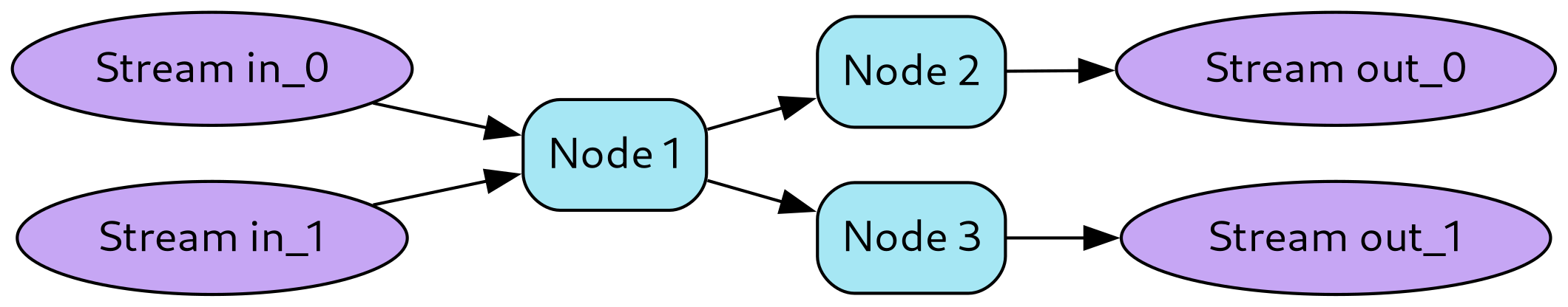
Source nodes are those that do not receive input from another node; examples include those that call out to external databases to generate output and those that generate synthetic data for testing or verification purposes. Sink nodes are those that do not emit output; examples include nodes that serialize results to disk and those that simply call out to an external service. An example of a node with multiple inputs is a join node, and an example of a node with multiple outputs is a splitter node that splits columns of its input into multiple sets across multiple streaming dataframes. 5.2. DAGs. In DataFlow, computational nodes are organized into a directed acyclic graph (DAG). In this sense, DataFlow may be interpreted as a dataflow programming paradigm, as the data (streaming dataframes) flows between nodes (computational operations). The DAG structure supports parallelism at the coarsest level. In particular, if neither node A nor node B is an ancestor of the other, then the two nodes may perform computation in parallel.

Formally, a DataFlow DAG is a directed acyclic graph G = (V, E) whose vertices v ∈ V are nodes (as above) and whose edges (u, v) ∈ E connect outputs of u to inputs of v. We write u ≺ v if there exists a directed path from u to v; this induces a partial order on V . Two nodes A, B ∈ V are concurrent if neither A ≺ B nor B ≺ A holds, in which case they may be scheduled in parallel in any topological ordering.

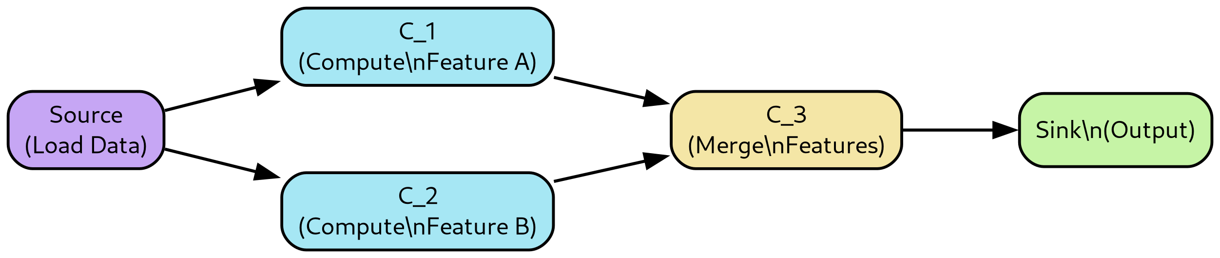
A simple DAG with 5 nodes, including one source and one sink, is depicted in Figure 5. Note that nodes C 1 and C 2 may be computed in parallel, as they have no dependency relationship. To determine the context window requirement of a DAG, we first formalize the context window of a path.

Let each node v ∈ V be point-in-time idempotent with a (minimal) context window length w v ∈ N. Consider a path p i 0 ,i 1 ,…,in = (v i 0 , v i 1 , . . . , v in ) from a source node v i 0 to a sink node v in . Definition 5.4 (Path context window). The context window w(p i 0 ,…,in ) of a path p i 0 ,…,in is defined as the minimal integer L such that the outputs at time t of v in depend only on the inputs at the source node v i 0 on the time interval [t -L + 1, t], for all t. Equivalently: if two executions of the DAG agree on all source-input stream values on [t -L + 1, t], then they produce identical outputs at time t at the sink along that path.

The following proposition shows that the formula used in DataFlow indeed computes this quantity.

Proposition 5.5 (Closed form for path context window). Let p i 0 ,i 1 ,…,in be a source-to-sink path in G, and let w i k be the context window of node v i k for k = 0, . . . , n. Then the path context window satisfies

Proof. We argue inductively on the length n of the path.

Base case n = 0. The path consists of a single node v i 0 with context window w i 0 . By definition of context window, the outputs at time t depend only on inputs on [t -w i 0 + 1, t], and this dependence is minimal. Thus w(p i 0 ) = w i 0 , which agrees with the formula 1 + (w i 0 -1).

Inductive step. Suppose the formula holds for all paths of length n -1, and consider a path p i 0 ,…,i n-1 ,in . Let p ′ denote its prefix (v i 0 , . . . , v i n-1 ), and write w(p ′ ) for the context window of p ′ . By the inductive hypothesis,

Consider the output of v in at time t. This depends on the outputs of v i n-1 on the time interval [t -w in + 1, t]. For each u ∈ [t -w in + 1, t], the output of v i n-1 at time u depends only on the inputs at v i 0 on the interval [u -w(p ′ ) + 1, u], by definition of w(p ′ ). The earliest time in this union, as u ranges over [t -w in + 1, t], is obtained by taking u = t -w in + 1 and then its left endpoint:

Hence the outputs of v in at time t depend only on inputs at v i 0 on the interval

Thus the context window w of path p i 0 ,i 1 ,…,in is given by

Note that the context window of a path of nodes each of context window 1 is itself 1. On the other hand, if p is a path of n context window-2 nodes, then the context window of p is n + 1, in accordance with the formula. This is due to the fact that, in proceeding backward along the path, the context window requirement for the current node is the union of the context window requirements of the output node; at each step, an additional time point enters into the context window requirement.

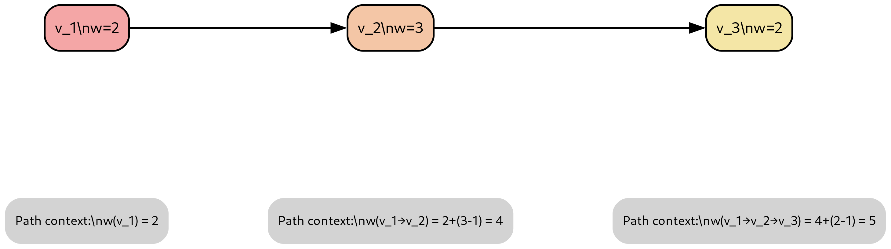
The following worked example illustrates the path context window calculation with concrete values.

Figure 6 illustrates this accumulation with a concrete example of a three-node linear chain. The context window w of a DAG G is the maximum of the context windows of all paths in G connecting a source node to a sink node:

Proposition 5.6 (Graph-level context window). Suppose every node v ∈ V in a DAG G is pointin-time idempotent with context window w v . Then:

(1) For each source-to-sink path p and each time t, the outputs at the sink node along p at time t depend only on the values of the source inputs on [t -w(p) + 1, t].

Consider a linear path

Timeline showing data dependencies:

To produce output at time t 0 , the path requires input data back to time t -4 . (2) The graph context window w(G) is the minimal integer L such that for every sink node and time t, the sink outputs at t depend only on the source inputs on [t -L + 1, t].

Proof. (1) is a direct consequence of Proposition 5.5, applied to each path separately. (2) follows because any influence from sources to a given sink must travel along some source-to-sink path. The largest window required among those paths is thus both sufficient (no path requires more than w(G) time steps) and necessary (for any smaller L < w(G), there exists a path whose sink output at time t can be changed by altering source inputs earlier than t -L + 1). □

Recall that the graph context window size is a lower bound for the minimum tile size. In many practical cases, conservative upper bounds for the graph context window size may be produced, which already may suffice for tiling purposes. Whether the estimated bounds suffice will depend upon the data, computational resources, and operational mode.

Proof. We construct a counterexample. Let G be a linear chain of nodes

Consider an input stream where all values are zero except for a single value of 1 at time t 0 = t -w(G) + 1. In streaming execution with full history, this input propagates through the chain and affects the output at time t. Specifically, by the definition of the graph context window, the output at time t depends on inputs back to time t -w(G) + 1 = t 0 . Now consider two-tile execution with tile length τ < w(G). The two tiles cover [t -2τ + 1, t]. Since 2τ < 2w(G), we have t -2τ + 1 > t -2w(G) + 1. In particular, if we choose the input spike at t 0 = t-w(G)+1, then t 0 > t-2τ +1 for τ < w(G) sufficiently small. However, the two-tile window [t -2τ + 1, t] does not extend back to t 0 , so the spike is not visible to the two-tile computation. The two-tile output at time t will be zero, while the streaming output is nonzero, demonstrating the disagreement.

More formally, choose τ = ⌊w(G)/2⌋ and set the spike at

so the spike falls outside the two-tile window, establishing the claim. □ Remark 5.9 (Practical implications of tile size selection). Proposition 5.8 establishes that τ ≥ w(G) is not merely sufficient but also necessary for correctness. In practice, this means that the tile size must be chosen based on the DAG’s context window. Choosing τ < w(G) leads to subtle errors where outputs appear correct for most time points but silently fail when context dependencies span tile boundaries. DataFlow’s testing framework detects such violations by comparing tiled and untiled execution across multiple random tile boundaries.

In DataFlow, the DAG topology is separated from the configuration of the nodes of the DAG, which we refer to as “DAG configuration”. For example, a machine learning node that fits and utilizes an autoregressive model may expose hyperparameters such as the order of the model (i.e., the number of lags to include), the technique used to learn parameters, and the model training period. A more pedestrian use case, common in practice, is to allow the user to define admissible node-level input and output column names of dataframes. We formalize this separation as follows.

Definition 5.10 (DAG topology and configuration). A DAG topology is a directed acyclic graph G = (V, E) together with, for each vertex v ∈ V ,

• its input and output arities (m v , n v ), and • its abstract node type (e.g. SISO, join, splitter, ML node), which fixes the input/output schema and the admissibility constraints (such as point-in-time idempotency and schema compatibility). A DAG configuration is a map κ : V -→ Conf, assigning to each node v a configuration object κ(v) that instantiates its type (e.g. concrete hyperparameters, column names, or pointers to user-defined functions).

A more abstract case is where the selection of computational operations is specified in the DAG configuration itself. For example, a computational node N may wrap a user-defined function conforming to some constraints on input and output schema. The wrapping may be implemented so that a pointer to the user-defined function is specified in the node configuration, thereby allowing the user to supply any function f which conforms to the constraints upon DAG configuration (or reconfiguration).

Formally, let UF v denote the set of all user-defined functions admissible at node v (e.g. those that satisfy the node’s schema constraints and point-in-time idempotency). Then a node configuration may include a choice f v ∈ UF v , and the overall DAG configuration is an element of the product space

where Conf v captures other node-specific parameters (such as lag order or training period for a model).

Remark 5.11 (Topology vs. configuration and context window). The DAG topology (V, E) encodes data dependencies and hence determines the way in which node-level context windows {w v } v∈V combine into the graph-level context window w(G). The DAG configuration κ selects concrete admissible functions at each node but does not change the topology. As long as the configured functions preserve the same node-level context windows, the graph context window w(G) remains unchanged when the DAG is reconfigured.

Associated with each node is a user-defined temporal minimum context window, which is used to impose a consistency requirement upon the computational node. Namely, provided the data window exceeds the context window, the latest-in-time output of the node must not depend upon the length of window provided. In other words, for the latest output, the node acts in an idempotent way over any data window of the streaming dataframe that includes the context window. We call this property point-in-time idempotency.

Performance bounds and scheduling. The explicit DAG structure in DataFlow enables analysis of performance bounds and scheduling opportunities. This section establishes fundamental limits on latency and parallelism. Theorem 5.12 (Critical-path latency lower bound). Let G = (V, E) be a DAG and let each node v ∈ V have service time τ (v) > 0 (the time required to process a single tile). The minimum possible latency to produce an output at a sink node is lower bounded by

the weighted length of the critical path in G.

Proof. Consider any source-to-sink path p = (v i 0 , v i 1 , . . . , v in ) where v i 0 is a source and v in is a sink. By the dependency structure of the DAG, node v i k cannot begin computation until all its predecessors have completed. In particular, along path p, node v i k cannot start until node v i k-1 has finished, which takes time at least τ (v i k-1 ).

Thus, the total time to compute the output at v in following path p is at least

Since the sink output depends on at least one source-to-sink path, and computation must proceed sequentially along any such path, the minimum latency is bounded below by the maximum path length. This maximum is the critical path.

Note that this bound is tight: a scheduler that processes nodes in topological order, with infinite parallelism across independent nodes, achieves exactly this latency. □ Remark 5.13 (Implications for system design). Theorem 5.12 establishes that the critical path length L * represents a fundamental lower bound on latency, independent of available computational resources. Even with infinite parallelism, latency cannot be reduced below L * . This has several practical implications:

• DAG restructuring for latency reduction. If a system fails to meet latency requirements, the only solution is to restructure the DAG to reduce the critical path length-either by optimizing slow nodes or by reorganizing dependencies to create shorter paths. • Resource allocation. Nodes on the critical path are candidates for priority resource allocation (e.g., GPU acceleration, caching), as improvements to non-critical nodes do not reduce overall latency. • Load balancing. In distributed execution, nodes on the critical path should be assigned to the fastest available workers to minimize end-to-end latency. Figure 8 illustrates these concepts with a Gantt chart comparing sequential and parallel execution.

Sequential Execution (1 processor):

Critical path: processors reduces total time to 10.5 units by executing v 3 and v 5 (blue) in parallel with critical path nodes (red). However, the critical path of 9 units remains the fundamental bottleneck. Nodes on the critical path (v 1 → v 2 → v 4 ) determine minimum latency regardless of parallelism.

Remark 5.14 (Parallelism and DAG width). The maximum instantaneous parallelism achievable in a DAG is upper bounded by the width of the DAG, defined as the size of the largest antichain (set of pairwise incomparable nodes in the partial order induced by the DAG). For a DAG with n nodes, total work W = v∈V τ (v), and critical path length L * , standard DAG scheduling results establish:

• The optimal makespan with P processors is at least max(L * , W/P ).

• Greedy topological scheduling achieves makespan at most L * + (W -L * )/P . In DataFlow, these bounds apply both to intra-tile parallelism (executing multiple nodes on the same time slice) and to inter-tile parallelism (processing multiple tiles concurrently). Definition 5.15 (DAG width and antichain). An antichain in a DAG G = (V, E) is a set A ⊆ V of nodes such that for any distinct u, v ∈ A, neither u ≺ v nor v ≺ u (i.e., they are incomparable in the partial order). The width of G is the size of the largest antichain. Proof. At any time step, the set of nodes currently executing forms an antichain (since if u ≺ v, then v cannot start until u completes). By definition, no antichain can have size exceeding w. □ Remark 5.17 (Amdahl’s law for DAGs). Even if most nodes in a DAG can be parallelized, the critical path imposes a serial bottleneck. This is analogous to Amdahl’s law: if fraction f of the work lies on the critical path, then the speedup with P processors is bounded by 1/(f + (1 -f )/P ), which approaches 1/f as P → ∞. For latency-critical applications, reducing the critical path fraction f is essential. For example, in a computation graph for a mathematical expression, nodes would represent operations like addition or multiplication, while edges would indicate the order (and grouping) of operations.

The DataFlow simulation kernel schedules nodes according to their dependencies.

6.3. Simulation kernel details. The most general case of simulation consists of multiple nested loops:

(1) Multiple DAG computation. The general workload contains multiple DAG computations, each one inferred through a Config belonging to a list of Configs describing the entire workload to execute.

• In this set-up each DAG computation is independent, although some pieces of computations can be common across the workload. DataFlow will compute and then cache the common computations automatically as part of the framework execution (2) Learning pattern. For each DAG computation, multiple train/predict loops represent different machine learning patterns (e.g., in-sample vs out-of-sample, cross-validation, rolling window)

• This loop accommodates the need for nodes with state to be driven to learn parameters and hyperparameters and then use the learned state to predict on unseen data (i.e., out-of-sample) (3) Temporal tiling. Each DAG computation runs over a tile representing an interval of time • As explained in section XYZ, DataFlow partition the time dimension in multiple tiles

• Temporal tiles might overlap to accommodate the amount of memory needed by each node (see XYZ), thus each timestamp will be covered by at least one tile. In the case of DAG nodes with no memory, then time is partitioned in non-overlapping tiles. • The tiling pattern over time does not affect the result as long as the system is properly designed (see XYZ) (4) Spatial tiling. Each temporal slice can be computed in terms of multiple sections across the horizontal dimension of the dataframe inputs, as explained in section XYZ.

• This is constrained by nodes that compute features cross-sectionally, which require the entire space slice to be computed at once (5) Single DAG computation. Finally a topological sorting based on the specific DAG connectivity is performed in order to execute nodes in the proper order. Each node executes over temporal and spatial tiles. Figure 9 illustrates the nested structure of these simulation loops. Note that it is possible to represent all the computations from the above loops in a single “scheduling graph” and use this graph to schedule executions in a global fashion.

Parallelization across CPUs comes naturally from the previous approach, since computations that are independent in the scheduling graph can be executed in parallel, as described in Section XYZ.

Incremental and cached computation is built-in in the scheduling algorithm since it’s possible to memoize the output by checking for a hash of all the inputs and of the code in each node, as described in Section XYZ.

Even though each single DAG computation is required to have no loops, a System (see XYZ) can have components introducing loops in the computation (e.g., a Portfolio component in a trading system, where a DAG computes forecasts which are acted upon based on the available funds). In this case, the simulation kernel needs to enforce dependencies in the time dimension. 6.4. Node ordering for execution. TODO(gp, Paul): Extend this to the multiple loop.

Topological sorting is a linear ordering of the vertices of a directed graph such that for every directed edge from vertex u to vertex v, u comes before v in the ordering. This sorting is only possible if the graph has no directed cycles, i.e., it must be a Directed Acyclic Graph (DAG). return post_order [:: -1] # Reverse the post -order to get the topological order 6.5. Heuristics for splitting computational steps into nodes. There are degrees of freedom in splitting the work between various nodes of a graph E.g., the same DataFlow computation can be described with several nodes or with a single node containing all the code

The trade-off is often between several metrics:

• Observability -More nodes make it easier to: * observe and debug intermediate the result of complex computation * profile graph executions to understand performance bottlenecks • latency/throughput -More nodes: * allows for better caching of computation * allows for smaller incremental computation when only one part of the inputs change * prevents optimizations performed across nodes * incurs in more simulation kernel overhead for scheduling * allows more parallelism between nodes being extracted and exploited • memory consumption -More nodes: * allows one to partition the computation in smaller chunks requiring less working memory

A possible heuristic is to start with smaller nodes, where each node has a clear function, and then merge nodes if this is shown to improve performance 6.6. DataFlow System. 6.6.1. Motivation. While DataFlow requires that a DAG should not have cycles, general computing systems might need to reuse the state from computation performed on past data. E.g., in a trading system, there is often a Forecast component that can be modeled as a DAG with no cycles and a Portfolio object that uses the forecasts to compute the desired allocation of capital across different positions based on the previous positions.

DataFlow supports this need by assembling multiple DAGs into a complete System that allows cycles.

The assumption is that DAGs are computationally expensive, while other components mainly execute light procedural computation that requires interaction with external objects such as databases, filesystems, sockets. In timed simulation (also referred to as historical, vectorized, or batch simulation), data is provided with an advancing clock that reports the current timestamp. The system enforces that only data with knowledge time less than or equal to the current timestamp is observable, thus preventing future peeking. This mode typically employs either a replayed clock or static clock depending on the specific use case.

Non-timed simulation. In non-timed simulation (also referred to as event-based or reactive simulation), the clock type is static. The wall-clock time corresponds to a timestamp equal to or greater than the latest knowledge time in the dataset. Consequently, all data in the dataframe becomes immediately available since each row has a knowledge time less than or equal to the wallclock time. In this mode, data for the entire period of interest is provided as a single dataframe.

For example, consider a system generating predictions every 5 minutes. In non-timed simulation, all input data are equally spaced on a 5-minute grid and indexed by knowledge time:

6.7.5. Real-time execution. In real-time execution, the clock type is a real clock. For a system predicting every 5 minutes, one forecast is generated every 5 minutes of wall-clock time, with data arriving incrementally rather than in bulk. 6.7.6. Replayed simulation. In replayed simulation, data is provided in the same format and timing as in real-time execution, but the clock type is a replayed clock. This allows the system to simulate real-time behavior while processing historical data, facilitating testing and validation of production systems. 6.7.7. Synchronous and asynchronous execution modes. Asynchronous mode. In asynchronous mode, multiple system components execute concurrently. For example, the DAG may compute while orders are transmitted to the market and other components await responses. The implementation utilizes Python’s asyncio framework. While true asynchronous execution typically requires multiple CPUs, under certain conditions (e.g., when I/O operations overlap with computation), a single CPU can effectively simulate asynchronous behavior.

Synchronous mode. In synchronous mode, components execute sequentially. For instance, the DAG completes its computation, then passes the resulting dataframe to the Order Management System (OMS), which subsequently executes orders and updates the portfolio.

The framework supports simulating the same system in either synchronous or asynchronous mode. Synchronous execution follows a sequential pattern: the DAG computes, passes data to the OMS, which then executes orders and updates the portfolio. Asynchronous execution creates persistently active objects that coordinate through mutual blocking mechanisms. 6.8. Vectorization.

6.8.1. Vectorization. Vectorization is a technique for enhancing the performance of computations by simultaneously processing multiple data elements with a single instruction, leveraging the capabilities of modern processors (e.g., SIMD (Single Instruction, Multiple Data) units). 6.8.2. Vectorization in DataFlow. Given the DataFlow format, where features are organized in a hierarchical structure, DataFlow allows one to apply an operation to be applied across the crosssection of a dataframe. In this way DataFlow exploits Pandas and NumPy data manipulation and numerical computing capabilities, which are in turns built on top of low-level libraries written in languages like C and Fortran. These languages provide efficient implementations of vectorized operations, thus bypassing the slower execution speed of Python loops. 6.8.3. Example of vectorized node in DataFlow. TODO 6.9. Incremental, cached, and parallel execution.

6.9.1. DataFlow and functional programming. The DataFlow computation model shares many similarity with functional programming:

• Data immutability: data in dataframe columns is typically added or replaced. A node in a DataFlow graph cannot alter data in the nodes earlier in the graph. • Pure functions: the output of a node depends only on its input values and it does not cause observable side effects, such as modifying a global state or changing the value of its inputs • Lack of global state: nodes do not rely on data outside their scope, especially global state 6.9.2. Incremental computation. Only parts of a compute graph that see a change of inputs need to be recomputed.

Incremental computation is an approach where the result of a computation is updated in response to changes in its inputs, rather than recalculating everything from scratch 6.9.3. Caching. Because of the “functional” style (no side effects) of data flow, the output of a node is determinstic and function only of its inputs and code.

Thus the computation can be cached across runs. E.g., if many DAG simulations share the first part of simulation, then that part will be automatically cached and reused, without needing to be recomputed multiple times.

Figure 10 shows the caching algorithm used by DataFlow. The framework enables loading DAG state for subsequent analysis. For instance, one might examine how linear model weights evolve over time in a rolling window simulation. 6.10.6. Batch computation and tiled execution. DataFlow supports batch computation through tiled execution, which partitions computation across temporal and spatial dimensions. Tiled execution provides several advantages:

• Memory efficiency: Large-scale simulations that exceed available memory can be executed by processing data in manageable tiles. • Incremental computation: Results can be computed progressively and cached, avoiding redundant calculations. • Parallelization: Independent tiles can be processed concurrently across multiple compute resources.

Temporal tiling. Temporal tiling partitions the time dimension into intervals. Each tile represents a specific time period (e.g., a single day or month). Tiles may overlap to accommodate node memory requirements. For nodes without memory dependencies, time is partitioned into non-overlapping intervals. Spatial tiling. Within each temporal slice, computation may be further divided across the horizontal dimension of dataframes. This approach is constrained by nodes that compute cross-sectional features, which require simultaneous access to the entire spatial slice. DAG runner implementations. Different DagRunner implementations support various execution patterns:

• FitPredictDagRunner: Implements separate fit and predict phases for in-sample and outof-sample evaluation. • RollingFitPredictDagRunner: Supports rolling window evaluation with periodic retraining. • RealTimeDagRunner: Executes nodes with real-time semantics, processing data as it arrives.

6.11. Backtesting and model evaluation. Backtesting provides a framework for evaluating model performance on historical data, supporting various levels of abstraction and fidelity to production environments. 6.11.1. Backtest execution modes. A backtest consists of code configured by a single Config object. The framework supports multiple execution modes:

• Batch mode: All data is available from the outset and processed in bulk, either as a single operation or partitioned into tiles. No clock advancement occurs during execution. • Streaming mode: Data becomes available incrementally as a clock advances, simulating real-time operation. This mode is equivalent to processing tiles with temporal span matching the data arrival frequency. • DagConfig: Contains node-specific parameters, excluding connectivity information which is specified in the DagBuilder. • SystemConfig: Encompasses the entire system specification, including market data configuration, execution parameters, and DAG configuration. • BacktestConfig: Defines temporal boundaries, universe selection, trading frequency, and data lookback requirements. Each configuration is serialized and stored alongside results, enabling precise reproduction of experiments.

6.12. Observability and debuggability. 6.12.1. Running a DAG partially. DataFlow allows one to run nodes and DAGs in a notebook during design, analysis, and debugging phases, and in a Python script during simulation and production phases.

It is possible to run a DAG up to a certain node to iterate on its design and debug. TODO: Add example 6.12.2. Replaying a DAG. Each DAG node can:

• capture the stream of data presented to it during either a simulation and real-time execution • serialize the inputs and the outputs, together with the knowledge timestamps • play back the outputs 7.5. Additional Related Systems. Several additional systems address specific aspects of distributed stream processing and machine learning but remain complementary to rather than competitive with DataFlow’s comprehensive approach. Apache Kafka Streams is a client library for building stream processing applications on top of Apache Kafka. The library provides stateful stream processing with exactly-once semantics but focuses on Kafka-centric architectures and does not provide integrated support for machine learning workflows or point-in-time idempotency guarantees.

Apache Samza is a distributed stream processing framework originally developed at LinkedIn. Samza integrates tightly with Apache Kafka for messaging and provides stateful stream processing capabilities. However, like Kafka Streams, it does not address the specific requirements of time series machine learning or provide formal temporal correctness guarantees.

Dask is a parallel computing library in Python that extends NumPy, pandas, and scikit-learn to distributed environments. While Dask supports dataframe operations and integrates well with the Python scientific computing ecosystem, it does not provide native streaming semantics, eventtime processing, or the temporal correctness guarantees required for time series machine learning applications. Dask is well-suited for batch processing of large datasets but does not address realtime streaming or causality validation.

MillWheel [1] is Google’s internal framework for fault-tolerant stream processing that inspired Apache Beam and Google Cloud Dataflow. The system introduced important concepts including persistent state and exactly-once processing semantics. However, MillWheel is an internal Google system and does not provide the ML-focused abstractions or Python-native programming model offered by DataFlow.

A comprehensive treatment of distributed data systems architecture and design patterns is provided by Kleppmann [5]. " " " Evaluate window size quality ( implementation detail ) . " " "

• Climate and Weather Analysis: Processing data from environmental sensors for weather prediction and climate research • Pollution Monitoring: Real-time tracking of air and water quality Gaming • In-Game Analytics: Real-time analysis of player behavior for game optimization and personalized experiences Social Media Analytics • Trend Analysis: Monitoring social media streams to identify and analyze trending topics and sentiments Emergency Response • Disaster Monitoring and Management: Real-time data analysis for effective response during natural or man-

t := [t -2τ + 1, t].

• We say that tiles C k and C ℓ are semantically identical if there exists a relabeling (e.g., of customers) under which F (k) [s,t] and F

• We can do a group-by or filter by full_symbol • Apply the transformation on each resulting dataframe • Merge the data back into a single dataframe with the □ Lemma 4.34 (Column-group-separable nodes). Let the columns decompose into disjoint groups C 1 , . . . , C m and suppose the node acts independently on each group with contexts w 1 , . . . , w m . Then the node is point-in-time idempotent with w = max j w j .Proof. For each group C j , the output at time t restricted to columns in C j depends only on inputs in C j over the window [t -w j + 1, t]. Since the computations are independent across groups, the overall output at time t depends on the union of these windows, which is [t -max j w j + 1, t]. Thus w = max j w j suffices. □ Lemma 4.35 (Joins with temporal alignment). Suppose two input streams are joined on time with left-closed, right-exact alignment and bounded misalignment ∆ ∈ N (e.g., last-observation-carriedforward up to ∆ time steps). If the input nodes are point-in-time idempotent with context windows w 1 and w 2 , then the join node is point-in-time idempotent with w = max(w 1 , w 2 ) + ∆.Proof. The join output at time t may depend on input values from either stream up to ∆ time steps earlier (due to the alignment tolerance). For each input stream i, we require access to [t -w i + 1, t] to compute its contribution. Accounting for the misalignment, we need access to [t -w i -∆ + 1, t].Taking the maximum over both streams yields w = max(w 1 , w 2 ) + ∆. □ 4.7. Approximating infinite impulse response operations. While finite impulse response (FIR) operations naturally satisfy point-in-time idempotency with bounded context windows, infinite impulse response (IIR) operations (such as exponential moving averages) technically require access to the entire history. In practice, IIR operations can be approximated by FIR operations with bounded truncation error.Theorem 4.36 (FIR approximation error for EWMA). Let y t+1 = (1 -λ)x t + λy t with 0 < λ < 1 define an exponentially weighted moving average (EWMA). Let ỹ(h) t be the truncated FIR approximation using the last h inputs:

• We can do a group-by or filter by full_symbol • Apply the transformation on each resulting dataframe • Merge the data back into a single dataframe with the □ Lemma 4.34 (Column-group-separable nodes). Let the columns decompose into disjoint groups C 1 , . . . , C m and suppose the node acts independently on each group with contexts w 1 , . . . , w m . Then the node is point-in-time idempotent with w = max j w j .Proof. For each group C j , the output at time t restricted to columns in C j depends only on inputs in C j over the window [t -w j + 1, t]. Since the computations are independent across groups, the overall output at time t depends on the union of these windows, which is [t -max j w j + 1, t]. Thus w = max j w j suffices. □ Lemma 4.35 (Joins with temporal alignment). Suppose two input streams are joined on time with left-closed, right-exact alignment and bounded misalignment ∆ ∈ N (e.g., last-observation-carriedforward up to ∆ time steps). If the input nodes are point-in-time idempotent with context windows w 1 and w 2 , then the join node is point-in-time idempotent with w = max(w 1 , w 2 ) + ∆.Proof. The join output at time t may depend on input values from either stream up to ∆ time steps earlier (due to the alignment tolerance). For each input stream i, we require access to [t -w i + 1, t] to compute its contribution. Accounting for the misalignment, we need access to [t -w i -∆ + 1, t].Taking the maximum over both streams yields w = max(w 1 , w 2 ) + ∆. □ 4.7. Approximating infinite impulse response operations. While finite impulse response (FIR) operations naturally satisfy point-in-time idempotency with bounded context windows, infinite impulse response (IIR) operations (such as exponential moving averages) technically require access to the entire history. In practice, IIR operations can be approximated by FIR operations with bounded truncation error.

• We can do a group-by or filter by full_symbol • Apply the transformation on each resulting dataframe • Merge the data back into a single dataframe with the □ Lemma 4.34 (Column-group-separable nodes). Let the columns decompose into disjoint groups C 1 , . . . , C m and suppose the node acts independently on each group with contexts w 1 , . . . , w m . Then the node is point-in-time idempotent with w = max j w j .Proof. For each group C j , the output at time t restricted to columns in C j depends only on inputs in C j over the window [t -w j + 1, t]. Since the computations are independent across groups, the overall output at time t depends on the union of these windows, which is [t -max j w j + 1, t]. Thus w = max j w j suffices. □ Lemma 4.35 (Joins with temporal alignment). Suppose two input streams are joined on time with left-closed, right-exact alignment and bounded misalignment ∆ ∈ N (e.g., last-observation-carriedforward up to ∆ time steps). If the input nodes are point-in-time idempotent with context windows w 1 and w 2 , then the join node is point-in-time idempotent with w = max(w 1 , w 2 ) + ∆.Proof. The join output at time t may depend on input values from either stream up to ∆ time steps earlier (due to the alignment tolerance). For each input stream i, we require access to [t -w i + 1, t] to compute its contribution. Accounting for the misalignment, we need access to [t -w i -∆ + 1, t].

• We can do a group-by or filter by full_symbol • Apply the transformation on each resulting dataframe • Merge the data back into a single dataframe with the □ Lemma 4.34 (Column-group-separable nodes). Let the columns decompose into disjoint groups C 1 , . . . , C m and suppose the node acts independently on each group with contexts w 1 , . . . , w m . Then the node is point-in-time idempotent with w = max j w j .Proof. For each group C j , the output at time t restricted to columns in C j depends only on inputs in C j over the window [t -w j + 1, t]. Since the computations are independent across groups, the overall output at time t depends on the union of these windows, which is [t -max j w j + 1, t]. Thus w = max j w j suffices. □ Lemma 4.35 (Joins with temporal alignment). Suppose two input streams are joined on time with left-closed, right-exact alignment and bounded misalignment ∆ ∈ N (e.g., last-observation-carriedforward up to ∆ time steps). If the input nodes are point-in-time idempotent with context windows w 1 and w 2 , then the join node is point-in-time idempotent with w = max(w 1 , w 2 ) + ∆.Proof. The join output at time t may depend on input values from either stream up to ∆ time steps earlier (due to the alignment tolerance). For each input stream i, we require access to [t -w i + 1, t] to compute its contribution. Accounting for the misalignment, we need access to [t -

• We can do a group-by or filter by full_symbol • Apply the transformation on each resulting dataframe • Merge the data back into a single dataframe with the □ Lemma 4.34 (Column-group-separable nodes). Let the columns decompose into disjoint groups C 1 , . . . , C m and suppose the node acts independently on each group with contexts w 1 , . . . , w m . Then the node is point-in-time idempotent with w = max j w j .Proof. For each group C j , the output at time t restricted to columns in C j depends only on inputs in C j over the window [t -w j + 1, t]. Since the computations are independent across groups, the overall output at time t depends on the union of these windows, which is [t -max j w j + 1, t]. Thus w = max j w j suffices. □ Lemma 4.35 (Joins with temporal alignment). Suppose two input streams are joined on time with left-closed, right-exact alignment and bounded misalignment ∆ ∈ N (e.g., last-observation-carriedforward up to ∆ time steps). If the input nodes are point-in-time idempotent with context windows w 1 and w 2 , then the join node is point-in-time idempotent with w = max(w 1 , w 2 ) + ∆.

• We can do a group-by or filter by full_symbol • Apply the transformation on each resulting dataframe • Merge the data back into a single dataframe with the □ Lemma 4.34 (Column-group-separable nodes). Let the columns decompose into disjoint groups C 1 , . . . , C m and suppose the node acts independently on each group with contexts w 1 , . . . , w m . Then the node is point-in-time idempotent with w = max j w j .

t □ Remark 4.37 (Approximate point-in-time idempotency). Theorem 4.36 justifies treating IIR operations as approximately point-in-time idempotent by selecting a truncation horizon h that achieves a target error tolerance ε. For example, with λ = 0.9 and ε = 10 -6 , we require h ≥ ln(10 6 ) ln(10/9) ≈ 131 time steps.

Theorem 4.43 (Causal safety with embargo). If all nodes are point-in-time idempotent and the system enforces causality with embargo ∆ such that all late arrivals satisfy k(u) ≤ u + ∆, then the embargoed execution is observationally equivalent to the ideal execution with no late data.Proof.By assumption, all data with logical time up to t arrives by wall-clock time t + ∆. The embargo ensures that outputs for logical time t are not emitted before wall-clock time t + ∆. Thus, at emission time, all relevant input data is available, and the computation proceeds identically to the ideal case where data arrives instantaneously at logical time. Point-in-time idempotency guarantees that the output at t depends only on the context window [t -w + 1, t], independent of when this data actually arrived (as long as it arrived before output emission). □ Proposition 4.44 (Detection of future-peeking). If a node uses data from time t + δ (where δ > 0)

Theorem 4.43 (Causal safety with embargo). If all nodes are point-in-time idempotent and the system enforces causality with embargo ∆ such that all late arrivals satisfy k(u) ≤ u + ∆, then the embargoed execution is observationally equivalent to the ideal execution with no late data.Proof.

Theorem 4.43 (Causal safety with embargo). If all nodes are point-in-time idempotent and the system enforces causality with embargo ∆ such that all late arrivals satisfy k(u) ≤ u + ∆, then the embargoed execution is observationally equivalent to the ideal execution with no late data.

6.7.4. Timed and non-timed simulation. Timed simulation.