Probing Scientific General Intelligence of LLMs with Scientist-Aligned Workflows

Figure 1 | Scientific General Intelligence (SGI) We define SGI as an AI that can autonomously navigate the complete, iterative cycle of scientific inquiry with the versatility and proficiency of a human scientist. The teaser illustrates the Practical Inquiry Model’s four quadrants-Deliberation (synthesis and critical evaluation of knowledge), Conception (idea generation), Action (experimental execution), and Perception (interpretation)-and how SGI-Bench operationalizes them through four task categories and an agent-based evaluation paradigm, together providing a principle-grounded, measurable framework for assessing scientific intelligence.

Large language models (LLMs) [1,2,3,4,5] are achieving and even exceeding human-level performance on a diverse array of tasks, spanning multidisciplinary knowledge understanding, mathematical reasoning, and programming. This rapid progress has ignited a vibrant debate: some view these models as early signals of artificial general intelligence (AGI) [6,7], whereas others dismiss them as mere “stochastic parrots [8],” fundamentally constrained by their training data. As these models evolve, the frontier of AGI research is shifting towards the most complex and structured of human endeavors: scientific inquiry [9]. We argue that demonstrating genuine scientific general intelligence (SGI) represents a critical leap toward AGI, serving as a definitive testbed for advanced reasoning, planning, and knowledge creation capabilities. However, much like AGI, the concept of SGI remains frustratingly nebulous, often acting as a moving goalpost that hinders clear evaluation and progress.

This paper aims to provide a comprehensive, quantifiable framework to cut through this ambiguity, starting with a concrete definition grounded in established theory:

To operationalize this definition, we ground our approach in the Practical Inquiry Model [10,11], a theoretical framework that deconstructs the scientific process into a cycle of four core cognitive activities. This model provides a taxonomic map of scientific cognition through four distinct, interdependent quadrants (Figure 1): Deliberation (the search, synthesis, and critical evaluation of knowledge), Conception (the generation of ideas), Action (the practical implementation via experiments), and Perception (the awareness and interpretation of results). An AI exhibiting true SGI must possess robust capabilities across this entire spectrum. This four-quadrant framework provides a conceptual taxonomy of scientific cognition and forms the foundation for an operational definition of SGI-one that specifies what kinds of planning, knowledge creation and reasoning an AI must demonstrate to qualify as scientifically intelligent. Translating this operational definition into measurable criteria requires examining how current evaluations of AI intelligence align with, or deviate from, this framework. Identifying these gaps is essential for clarifying what existing assessments capture and what they overlook in defining Scientific General Intelligence.

Grounded in this four-quadrant definition of SGI, we examine how existing benchmarks operationalize scientific reasoning. Most current evaluations capture only fragments of the SGI spectrum. For instance, MMLU [12] and SuperGPQA [13] focus on multidisciplinary knowledge understanding-corresponding mainly to the Deliberation quadrant-while GAIA [14] emphasizes procedural tool use aligned with Action. HLE [15] further raises difficulty through complex reasoning, yet still isolates inquiry stages without integrating the practical or interpretive cycles that characterize real scientific investigation. Collectively, these benchmarks present a fragmented view of scientific intelligence. Their disciplinary scope remains narrow, their challenges seldom reach expert-level reasoning, and-most crucially-they frame inquiry as a static, closed-domain question-answering task. This abstraction neglects the creative, procedural, and self-corrective dimensions central to SGI, meaning that what is currently measured as “scientific ability” reflects only a limited slice of true Scientific General Intelligence.

Thus, to concretize the proposed definition of Scientific General Intelligence (SGI), we develop SGI-Bench: A Scientific Intelligence Benchmark for LLMs via Scientist-Aligned Workflows. Rather than serving as yet another performance benchmark, SGI-Bench functions as an operational instantiation of the SGI framework, quantitatively evaluating LLMs across the full spectrum of scientific cognition defined by the Practical Inquiry Model. By design, SGI-Bench is comprehensive in its disciplinary breadth, challenging in its difficulty, and unique in its explicit coverage of all four capabilities central to our definition of SGI. The benchmark structure is therefore organized into four corresponding task categories:

• Building upon our theoretical framework, the construction of SGI-Bench operationalizes the proposed definition of Scientific General Intelligence (SGI). We began with foundational topics drawn from Science’s 125 Big Questions for the 21st Century [16], spanning ten major disciplinary areas. Through multi-round collaborations with domain experts, we identified high-impact research problems and curated raw source materials from leading journals such as Nature, Science, and Cell. Together with PhD-level researchers, we implemented a multi-stage quality control pipeline involving human annotation, model-based verification, and rule-based consistency checks. The resulting benchmark comprises over 1,000 expert-curated samples that concretely instantiate the reasoning, creativity, and experimental competencies central to our definition of SGI.

To evaluate performance across these four dimensions, we found that conventional “LLM-as-ajudge” [17] paradigms are insufficient to handle the diverse and specialized metrics required by SGI assessment. To address this, we developed an agent-based evaluation framework following an Agent-as-a-judge [18] paradigm. Equipped with tools such as a web search interface, Python interpreter, file reader, PDF parser, and discipline-specific metric functions, this framework ensures rigor, scalability, and transparency. It operates through four interdependent stages-Question Selection, Metric Customization, Prediction & Evaluation, and Report Generation-each coordinated by specialized agents aligned with different aspects of scientific inquiry.

Applying SGI-Bench to a wide spectrum of state-of-the-art LLMs reveals a unified picture: while modern models achieve pockets of success, they fall far short of the integrated reasoning required for scientific intelligence.

• In deep scientific research, models can retrieve relevant knowledge but struggle to perform quantitative reasoning or integrate multi-source evidence; exact-match accuracy remains below 20% and often collapses on numerical or mechanistic inference. • In idea generation, models show substantial deficits in realization. This manifests in underspecified implementation steps and frequent proposals that lack actionable detail or fail basic feasibility checks. • In dry experiments, even strong models fail on numerical integration, simulation fidelity, and scientific code correctness, revealing a gap between syntactic code fluency and scientific computational reasoning. • In wet experiments, workflow planning shows low sequence similarity and error-prone parameter selection, with models frequently omitting steps, misordering actions, or collapsing multi-branch experimental logic. • In multimodal experimental reasoning, models perform better on causal and perceptual reasoning but remain weak in comparative reasoning and across domains such as materials science and earth systems. • Across tasks, closed-source models demonstrate only a marginal performance advantage over open-source models. Even the best closed-source system achieves an SGI-Score of around 30/100, reflecting that current AI models possess relatively low capability in multi-task scientific research workflows, and remain far from proficient for integrated, real-world scientific inquiry.

Collectively, these findings demonstrate that current LLMs instantiate only isolated fragments of scientific cognition. They remain constrained by their linguistic priors, lacking the numerical robustness, procedural discipline, multimodal grounding, and self-corrective reasoning loops essential for scientific discovery.

Because genuine scientific inquiry is inherently open-ended and adaptive, we further explore how SGI may emerge under test-time learning dynamics. Preliminary experiments using test-time scaling [19] and reinforcement learning [20] suggest that models can enhance hypothesis formation and reasoning through minimal unlabeled feedback. This adaptive improvement provides empirical support for viewing Scientific General Intelligence not as a static property, but as a dynamic capacity that can evolve through iterative, self-reflective reasoning cycles.

In summary, this work provides a principle-grounded definition of Scientific General Intelligence (SGI) and a corresponding framework for its empirical study. By formalizing the cognitive cycle of scientific inquiry and operationalizing it through SGI-Bench, we clarify what it means for an AI to exhibit scientific intelligence in both theory and practice. While not a final answer, this definition establishes a concrete path for future research-linking conceptual understanding with measurable progress toward AI systems capable of genuine scientific reasoning and discovery.

Scientific General Intelligence (SGI) refers to an AI system capable of engaging in the full cycle of scientific inquiry with autonomy, versatility, and methodological rigor. Unlike systems that excel at isolated reasoning tasks, an SGI-capable model must integrate knowledge retrieval, idea formation, action execution, and evidence-based interpretation into a coherent, iterative workflow.

To formalize this notion, we characterize scientific cognition through four interdependent stages: Deliberation (evidence search, synthesis, and critical assessment), Conception (generation of hypotheses and ideas), Action (implementation of experiments or simulations), and Perception (interpretation of empirical results).

Grounded in this framework, we provide an operational definition: an AI system exhibits SGI if it can (1) retrieve, synthesize, and critically evaluate knowledge; (2) generate scientifically grounded and novel ideas; (3) plan and execute experimental procedures; (4) interpret empirical outcomes with causal and contextual awareness.

This definition highlights a central limitation in existing benchmarks [12,13,14,15]: most evaluate factual recall or single-step reasoning, but few examine the structured, long-horizon workflows that constitute real scientific inquiry.

Building on the operational definition of SGI established in the previous section, we introduce SGI-Bench (Scientific Intelligence Benchmark for LLMs via Scientist-Aligned Workflows) -a benchmark designed to empirically evaluate the extent to which large language models (LLMs), vision-language models (VLMs), and agent-based systems exhibit the cognitive and procedural abilities required for scientific discovery. SGI-Bench systematically measures AI performance across 10 core scientific domains -astronomy, chemistry, earth science, energy, information science, life science, materials science, neuroscience, physics and math -providing a panoramic view of how AI systems engage with scientific reasoning across disciplines. Its task design draws inspiration from the seminal article 125 Questions: Exploration and Discovery [16] published in Science, ensuring both disciplinary breadth and societal relevance.

At the heart of SGI-Bench lies the principle of scientist alignment-the commitment to evaluating models under conditions that authentically mirror real scientific workflows. This concept manifests in several ways:

• The task designs closely mirror the real-world research scenarios encountered by scientists in their work, ensuring that each task is intrinsically tied to the scientific discovery process. • The raw materials used in task construction are sourced directly from scientists, ensuring the authenticity and relevance of the content. • Scientists have been closely involved in the process of constructing the benchmark, with a scientist-in-the-loop approach, ensuring the tasks reflect the nuances of actual scientific workflows. • The final evaluation scores are aligned with the checklist based on the needs of real scientific research scenarios from scientists, which ensures that the assessments genuinely reflect the scientific utility of the models.

SGI-Bench departs from conventional benchmarks that emphasize factual recall or single-turn reasoning. Instead, it operationalizes the long-horizon workflow of scientific discovery into four interdependent stages: literature review(Deliberation), methodology design(conception), experiment implementation(Action), and experimental analysis(Perception). These stages correspond to fundamental capabilities required of AI systems: information integration and understanding(Scientific Deep Research), design and planning(Idea Generation), experimental execution(Dry/Wet Experiment), and reasoning-based interpretation(Experimental Reasoning). Together, they form a unified framework that measures not only what models know but how they think, plan, and adapt in pursuit of new knowledge.

Scientific deep research refers to a thorough and comprehensive investigation of a specific scientific topic, combining elements of both AI-driven deep research [21,22,23] and scientific meta-analysis [24,25]. This task typically involves multi-step reasoning, web searches, document retrieval, and data analysis [26,27,28]. Drawing inspiration from AI’s deep research, which often relies on multihop searches to gather diverse information across multiple sources [29], it also incorporates the methodology of meta-analysis from the scientific community. Meta-analysis, a rigorous form of scientific research, synthesizes existing literature to derive precise, data-driven conclusions and extract quantitative insights from a large body of studies. Unlike general deep research, which may focus on qualitative understanding, meta-analysis centers on aggregating and analyzing data to produce statistically significant results. By combining the multi-hop search nature of AI’s deep research with the systematic, evidence-based approach of meta-analysis, this task ensures results that are both scientifically precise and meaningful. The ability to perform scientific deep research is crucial for advancing scientific knowledge, as it enables AI models to replicate the process of reviewing, synthesizing, and analyzing existing research to formulate new, data-driven hypotheses. [30,31] Deep Research comprises multiple forms including literature inquiry [32], report-style reasoning [33] and so on. In this benchmark, we focus on literature-inquiry-centric deep research, where the model identifies and integrates relevant scientific knowledge from provided sources. This process often involves unit verification, quantitative interpretation, and causal assessment-abilities fundamental to scientific reasoning and still challenging for current AI systems. By constraining the task to literature Table 1 | Scientific Deep Research Types: Four representative categories of inquiry targets and their roles in the scientific workflow.

Data Focused on retrieving or analyzing structured datasets, such as event counts, statistical summaries, or dataset-specific attributes.

Supports quantitative literature review and provides a foundation for identifying trends or anomalies.

Concerned with identifying or inferring material, molecular, or system properties, often requiring interpretation of experimental results or theoretical knowledge.

Bridges literature review with methodology design by clarifying key parameters.

Micro-experiment Small-scale controlled experiments, often involving chemical reactions, physical transformations, or laboratory processes under specific conditions.

Provides simulated reasoning over experimental procedures and outcomes.

Macro-experiment Large-scale or natural experiments, such as astronomical events, climate observations, or geophysical phenomena.

Extends literature review to global or long-term observations, anchoring hypotheses in real-world contexts.

• Background (B): A detailed background of the research topic, including the scientific field and subfields, to avoid ambiguities in terminology. • Constraints (C): Constraints such as experimental settings, scientific assumptions, and data sources that frame the problem appropriately. • Data (D): Any experimental or empirical data directly mentioned in the task, which might be either explicitly provided or inferred. • Question (Q): A specific, focused question that the task aims to address, such as determining a particular quantity or its variation over time. • Response Requirements (R): Specifications for the answer, including the required units and whether the answer should be an integer or a decimal with a specified number of decimal places.

• Steps (S): A detailed, step-by-step approach that the system uses to retrieve and process data or perform reasoning. • Answer (A): A precise numerical or string-based response, such as a specific value or a phrase.

S, A = LLM/Agent(B, C, D, Q, R)

Figure 3 | Scientific Deep Research Task: Inputs, outputs, and formulation for literature-driven quantitative inquiry combining multi-step reasoning and meta-analysis.

Idea generation is a critical component of the scientific process, corresponding to the stage of research methodology design. At this stage, researchers synthesize existing knowledge, engage in associative and creative thinking, and propose new approaches to address current challenges. It embodies the creative essence of scientific inquiry and shapes the direction and potential impact of subsequent research.

In real-world scientific workflows, idea generation typically occurs after researchers have completed a thorough literature review. They integrate prior findings, identify limitations or knowledge gaps, and use creative reasoning to formulate new hypotheses, methods, or frameworks aimed at overcoming these shortcomings. In this sense, idea generation serves as the crucial link between literature understanding and methodological innovation.

However, because idea generation is an open-ended and highly creative task, its evaluation is inherently challenging. In principle, scientific ideas span a wide spectrum from high-level hypotheses to fully specified methodological plans [34,35,36]. Evaluating the quality of open-ended hypotheses-those with substantial conceptual freedom and without explicit implementation structure-requires extensive human expert review to achieve even a modest degree of inter-rater reliability and public defensibility. Such large-scale expert adjudication is beyond the practical scope of this version of the benchmark.

Consequently, our current Idea Generation evaluation focuses on the methodological-design component of an idea-i.e., how a proposed approach is operationalized through data usage, step-by-step procedures, evaluation protocols, and expected outcomes. This component offers a more constrained structure that enables measurable, partially automatable assessment while still reflecting an essential aspect of scientific ideation. We view this as a pragmatic starting point, and future versions of the benchmark may incorporate broader hypothesis-level evaluation once sufficiently robust expert-sourced ground truth becomes feasible.

To make the assessment more systematic and tractable, we decompose an originally holistic idea into several interrelated components, forming a structured representation of the idea. This decomposition enables more fine-grained evaluation along dimensions such as effectiveness, novelty, level of detail, and feasibility [37].

Task Input

• Related Work (RW): A summary of existing research relevant to a certain research direction, providing context for new ideas. • Challenge (C): The current challenges in the field and the limitations of existing solutions. • Limitation (L): Specific shortcomings or constraints of current research that new ideas need to address. • Motivation (M): The perspective and motivation of addressing the limitations in this research direction. • Task Objective (TO): The primary goal of the task, such as generating ideas that solve identified challenges or improve existing solutions.

• Existing Solutions (ES): A description of the current approaches or solutions available in the field.

• Core Idea (CI): The central novel idea or concept generated to address the research challenge. • Implementation Steps (IS): The steps or procedures required to implement the core idea. • Implementation Order (IO) : The sequence in which the implementation steps should be executed. • Data (D) : The data that will be used to implement the idea or evaluate its effectiveness.

• Evaluation Metrics (EM): The criteria for assessing the success or relevance of the generated idea. • Expected Outcome (EO): The anticipated result or contribution the idea is expected to achieve.

CI, IS, IO, D, EM, EO = LLM/Agent(RW, C, L, M, TO, ES)

Figure 4 | Idea Generation Task: Inputs, outputs, and formulation for methodology design, integrating evaluation metrics and structured implementation planning.

Scientific experimentation represents the core of the discovery process, bridging theoretical formulation and empirical validation [30]. Within SGI-Bench, we formalize this process into two complementary categories: dry and wet experiments. Dry experiments capture computational and simulation-based studies-where AI assists in generating, refining, or executing scientific code that models physical phenomena. [38,39] Wet experiments, by contrast, simulate laboratory-based workflows, requiring the model to plan and reason about sequences of actions involving physical instruments, reagents, and procedural parameters [40,41]. Together, these two categories span the continuum from theoretical abstraction to empirical realization, offering a holistic evaluation of how AI can assist scientists in both virtual and physical experimentation.

Computational and laboratory experiments take many forms in real scientific practice. For dry experiments, possible tasks range from full pipeline construction to simulation design and multimodule scientific computing; in this benchmark, we adopt a code-completion-based formulation [42], where the model fills in missing components of an existing scientific script rather than generating an entire project from scratch. For wet experiments, laboratory workflows span diverse operational activities, yet we focus on the protocol-design aspect [43], where the model composes a sequence of experimental actions and parameters from a predefined action space.

By constraining dry and wet experiments to code completion and protocol design respectively, we retain core aspects of computational and laboratory reasoning while ensuring reproducibility, controlled variability, and reliable evaluation across models.

Dry experiments emphasize computational problem-solving, reflecting the growing role of AI in automating simulation-driven science. Each task presents the model with incomplete or masked scientific code that encapsulates domain-specific computations, such as molecular dynamics, climate modeling, or numerical solvers in physics [44]. The model must infer the missing logic, reconstruct executable code, and ensure that the resulting program produces correct and efficient outcomes. This task thus evaluates a model’s ability to integrate scientific understanding with code synthesis-testing not only syntactic correctness but also conceptual fidelity to the underlying scientific problem [42].

To better characterize the scope of dry experiments, we categorize representative computational functions commonly encountered across disciplines, including numerical calculation, statistical analysis, simulation, metric calculation, data processing, and predictive modeling, as shown in Table 2. The completion or generation of these functions offers a rigorous measure of how well AI systems can operationalize scientific intent into executable form.

Table 2 | Dry Experiment Function Types: Representative computational functions and their roles across scientific code-completion tasks.

Numerical Calculation Basic mathematical computations required to support physical or chemical modeling.

Processing experimental data using descriptive or inferential statistics to identify trends and distributions.

Running computational simulations (e.g., molecular dynamics, finite element analysis) and filtering results for relevant conditions.

Computing evaluation metrics such as accuracy, error, or performance indicators for validating experiments.

Handling raw data before and after experiments, including normalization, cleaning, and feature extraction.

Applying machine learning methods to categorize, predict, or group experimental results.

In real scientific workflows, dry experiments correspond to the stage of experimental design in computational and simulation-based studies. Following hypothesis formulation, researchers employ virtual experiments to anticipate and evaluate potential outcomes prior to empirical validation, enabling a cost-efficient and theoretically grounded pre-assessment of experimental feasibility.

• Background (B): Information from relevant scientific code, providing context for the dry experiment. • Data Code (D): The data used in the experiment, including any code snippets or predefined inputs. • Main Code (M): The core experimental code where some functions may be masked or missing.

• Functions (F): The missing functions in the main code 𝑀, which the system is tasked with generating or completing.

Task Formulation F = LLM/Agent(B, D, M)

Figure 5 | Dry Experiment Task: Inputs, outputs, and formulation for code-completion based computational studies with masked functions.

Wet Experiment Wet experiments represent the physical realization of scientific inquiry, encompassing laboratory and field-based procedures that transform theoretical designs into empirical evidence. These tasks simulate the execution phase of real-world experiments, where models are required to plan, organize, and reason through sequences of atomic actions involving materials, instruments, and procedural parameters. Given inputs describing experimental objectives, configurations, and available tools, the model must generate structured, executable protocols that are both accurate and practically feasible. Evaluation considers not only the correctness of individual steps but also their procedural coherence and alignment with established laboratory conventions.

In real scientific workflows, wet experiments correspond to the execution and validation stages of discovery. This is where hypotheses are tested against the physical world, data are collected, and evidence is generated to confirm, refine, or refute prior assumptions. By assessing how effectively AI systems can design and reason through these embodied experimental processes, this task provides a window into their capacity to bridge symbolic understanding with real-world scientific practice.

• Background (B): Information from relevant experimental procedure.

• Action Pool (AP): A predefined set of atomic actions that can be used in the experiment, along with explanations and corresponding input/output definitions.

• Atomic Action Order (AAO): The order in which atomic actions should be executed. • Atomic Action Parameters (AAP): The parameters associated with each atomic action (e.g., reagents, temperature).

AAO, AAP = LLM/Agent(B, AP)

Figure 6 | Wet Experiment Task: Inputs, outputs, and formulation for laboratory protocol planning via atomic actions and parameters.

Experimental reasoning refers to the process of interpreting scientific observations and data to reach justified conclusions. In this benchmark, we focus on data-analysis-oriented reasoning [45], where the model must extract relevant visual or numerical cues from multi-modal sources [46], compare conditions, and identify causal or descriptive patterns. This formulation emphasizes analytical interpretation rather than open-form scientific narrative, enabling reliable assessment while capturing an essential part of empirical scientific reasoning.

We consider five representative modalities as shown in Table 3: a) process images that integrate symbolic and textual information to depict workflows or variable relationships; b) observation images representing raw data captured by instruments such as telescopes, satellites, or microscopes; c) experiment images documenting laboratory setups and procedures; d) simulation images generated by computational models to visualize physical or chemical processes; and e) visualization images such as plots or charts that reveal patterns within structured datasets. Collectively, these modalities reflect the multi-faceted and evidence-driven nature of scientific inquiry. Identifying patterns in telescope images or microscope slides.

Attribute Understanding Requires disciplinary background to interpret key features and scientific attributes.

Recognizing crystalline structures in materials science images.

Comparative Reasoning Integrates and contrasts information across multiple images, often crossdomain.

Comparing climate model simulations with satellite observations.

Goes beyond correlation to infer mechanisms or propose hypotheses.

Inferring causal pathways in gene expression from multi-modal experimental data.

requires reasoning or analysis.

• Reasoning (R): The specific steps in the reasoning process, including calculation, thinking, analysis, etc.. • Answer (A): The conclusion drawn from analyzing the experimental data, answering the specified question or hypothesis.

R, A = LLM/Agent(MEI, Q)

Figure 7 | Experimental Reasoning Task: Inputs, outputs, and formulation for multi-modal analysis with step-by-step reasoning and final answers.

To align with the scientific characteristics of each task, we have designed multi-dimensional evaluation metrics for every task. This approach avoids a one-size-fits-all binary judgment and instead provides a more fine-grained assessment.

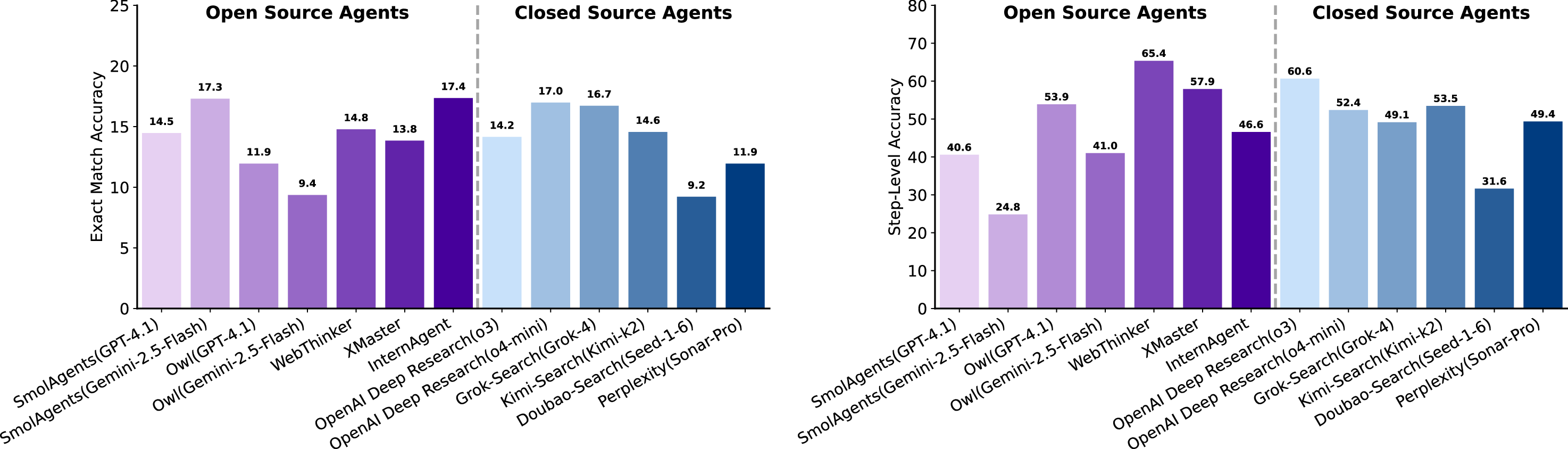
The Scientific Deep Research task draws inspiration from AI’s deep research paradigms [47,48,49,50,51] while incorporating methodologies from meta-analysis in the scientific domain. The former emphasizes multi-step reasoning, where solving a problem often requires iterative searches, calculations, and inferences; the correctness of each step directly impacts the accuracy of the final answer. The latter focuses on systematically extracting and synthesizing data from literature, requiring highly precise results. Accordingly, our metrics capture both step-by-step reasoning fidelity and final answer accuracy.

Exact Match (EM): Since the Scientific Deep Research tasks are designed to have short, unique, and easily verifiable answers, we use exact match as a hard metric to assess whether the model’s final answer is correct. The model receives a score of 1 if the output exactly matches the reference answer, and 0 otherwise.

Step-Level Accuracy (SLA): Models are required to produce step-by-step solutions. We employ an LLM-based judge to compare each model-generated step against the reference solution steps. For each step, the judge determines whether it is correct and provides reasoning. This fine-grained evaluation avoids binary correctness judgments for the entire solution, allowing precise assessment of reasoning accuracy at each inference step. The metric is computed as the proportion of steps correctly solved relative to the total number of steps. The score is calculated as SLA = Number of correct reasoning steps Total number of reasoning steps .

To evaluate the open-ended nature of idea generation, we adopt a hybrid framework that integrates both subjective and objective metrics. We assess each idea along four dimensions-effectiveness, novelty, detailedness, and feasibility-which together characterize an idea’s scientific quality, creativity, and executability [37,52].

Subjective Evaluation via LLM Judges. For subjective scoring, we perform pairwise comparisons between model-generated ideas and expert-written reference ideas. For each of the four dimensions, an LLM judge selects which idea is superior. To ensure fairness and robustness, we employ three different LLM judges, each casting two independent votes, resulting in a total of six votes per dimension. The pairwise win rate against the reference idea is then used as the subjective component of the score for each dimension.

Objective Evaluation via Computable Metrics. In addition to subjective judgments, we design dimension-specific computational metrics that capture structured properties of the ideas.

For each reference idea, human experts extract its 3-5 most essential keywords. We compute the hit rate of these keywords in the model-generated idea, allowing semantic matches to avoid underestimating effectiveness. The final effectiveness score is the average of the keyword hit rate and the LLM-judge win rate:

.

We measure novelty by computing the dissimilarity between the model-generated idea and prior related work. Lower similarity indicates that the model proposes ideas not present in existing literature and therefore exhibits higher creativity. .

For each research direction, domain experts provide a standardized implementation graph containing the essential nodes and their execution order. We extract an implementation graph from each model-generated idea and compute its similarity to the expert template. A low similarity indicates that the proposed idea does not align with accepted solution workflows and is therefore infeasible. The final feasibility score is:

Taken together, the hybrid subjective-objective design provides a robust, interpretable, and comprehensive assessment of LLMs’ scientific idea generation capabilities across creativity, structural clarity, and practical executability.

Dry Experiment Dry experiments focus on code generation task. Specifically, each problem includes background information, data code, and main code with certain functions masked. The model is tasked with completing the missing functions. Each problem contains 5 unit tests. Our metrics capture both correctness and execution behavior of the generated code [53]. the number of discordant pairs between the sequences. For sequences of length 𝑛, the score is computed as:

,

where 𝑛(𝑛-1)

is the maximum possible number of inversions. By definition, SS = 1 indicates that the sequences are identical, while SS = 0 indicates maximal disorder relative to the reference sequence.

Parameter Accuracy (PA): This metric measures the correctness of input parameters for each atomic action compared to the reference, including reagent types, concentrations, volumes, or other domain-specific parameters. The score is calculated as the proportion of correctly specified parameters across all actions: PA = Number of correctly specified parameters Total number of parameters .

The Experimental Reasoning task assesses the multi-modal scientific reasoning capabilities of LLMs and agents. Specifically, given several images and a corresponding question, the model is required to select the correct option from no fewer than 10 candidates. For evaluation, the correctness of the final answer and the validity of intermediate reasoning are equally critical. Therefore, two evaluation metrics are adopted, as detailed below.

Multi-choice Accuracy (MCA): Given several options, the model receives a score of 1 if the selected option exactly matches the reference answer, and 0 otherwise. The final score of MCA is the average of all individual scores across all test samples. This metric directly quantifies the model’s ability to pinpoint the correct solution from a large candidate pool, serving as a foundational measure of its end-to-end scientific reasoning accuracy in the multi-modal task.

Reasoning Validity (RV): Models are required to generate step-by-step logical reasoning to justify their selected answers. An LLM-based judge is utilized to assess the model-generated reasoning against a reference reasoning. For each test sample, the LLM judge assigns a validity score ranging from 0 (completely invalid, contradictory, or irrelevant) to 10 (fully rigorous, logically coherent, and perfectly aligned with the reference reasoning), accompanied by justifications for the assigned score. This fine-grained scoring paradigm circumvents the limitations of binary correctness assessments, enabling precise quantification of reasoning quality, including the validity of premises, logical transitions, and alignment with scientific principles. The final RV score is computed as the mean of individual sample scores across the entire test set, reflecting the model’s overall capability to perform interpretable and reliable scientific reasoning.

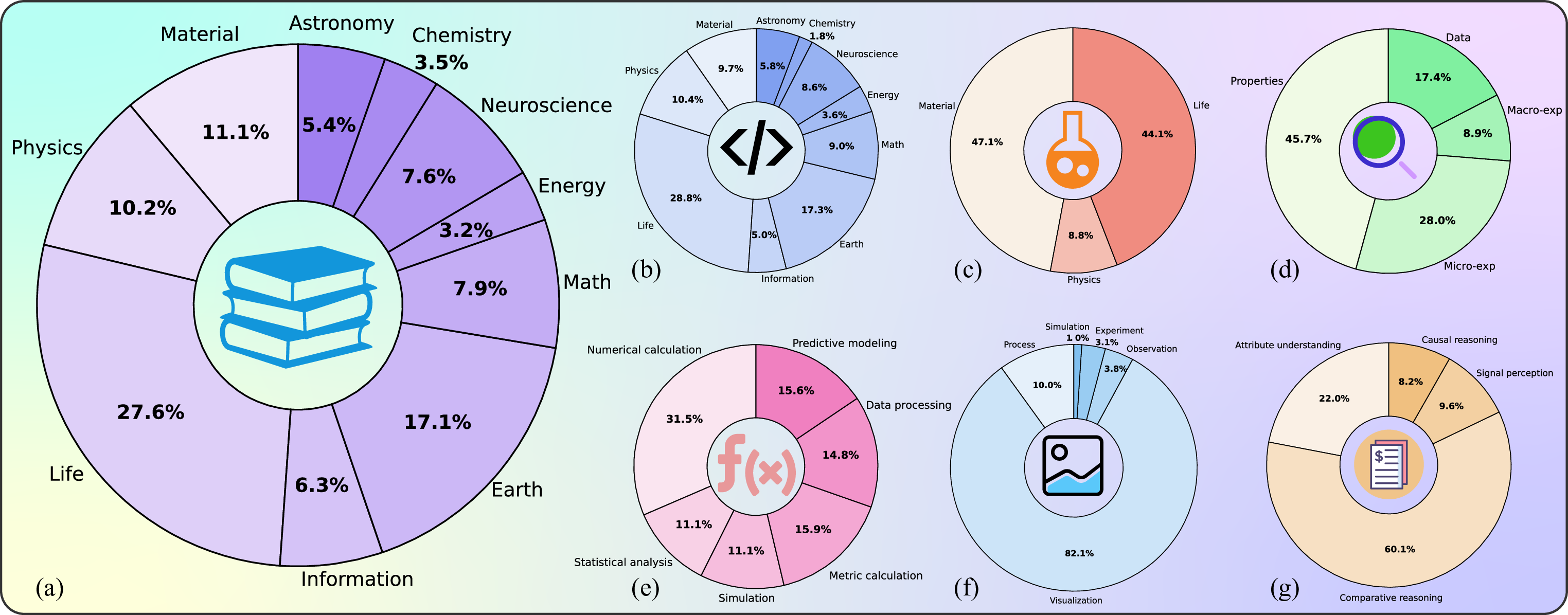
Raw Corpus Collection In this stage, we conducted multiple discussions with experts from diverse scientific disciplines, drawing from both the 125 important scientific questions published in Science, and the prominent research directions in various disciplines with significant scientific impact. Ultimately, we curated 75 research directions spanning ten scientific domains, as shown in Figure 8. Please refer to Appendix A.2 for a complete list of research directions.

Subsequently, we collected raw data provided by experts and researchers, primarily consisting of scientific texts and images across the various disciplines. The texts mainly cover knowledge introduction, methodological design, experimental procedures, and data analysis. The images include experiment figures, data visualizations, and observational images, each accompanied by detailed descriptions.

In addition, these experts and researchers will provide seed questions and annotation requirements for annotation, which provide initial examples for the subsequent annotation process, as illustrated in Figure 2 (G).

After gathering the raw data, we recruited over 100 Master’s and PhD holders from different disciplines to construct benchmark questions according to the task definitions. Annotators first analyzed the collected texts and images, and then created questions according to annotation requirements and seed questions. Several rules were applied to ensure scientific validity and authenticity. Specifically, annotators were required to reference the original data source and paragraph for each question, ensuring traceability to scientist-provided data. Furthermore, all questions are constructed by at least two annotators, one of whom is responsible for generating complex draft questions, and the other is responsible for refining them, as shown in Figure 2 (G).

During question construction, experts continuously reviewed the generated questions. Each question was immediately submitted to the relevant expert for evaluation, who assessed its scientific value.

For instance, a question with an experiment configuration that lacks general applicability would be deemed scientifically invalid. Experts provided feedback to annotators, who then revised the questions accordingly, ensuring that the constructed questions remain aligned with the perspectives and standards of domain scientists.

Data Cleaning Once all questions were constructed, we applied three layers of data cleaning: 1.

Rule-based cleaning: Questions that did not meet task-specific criteria were removed. For example, for Scientific Deep Research, steps must be short sentences forming a list, each representing one step; for Wet Experiments, each action must exist in the predefined action pool. 2. Model-based cleaning: Large language models were used to detect and remove questions with semantic errors or potential logical inconsistencies. 3. Expert quality check: All questions were reviewed by the original data-providing scientists, removing incomplete questions, questions with non-unique answers, or questions whose research direction did not align with the source data. For Dry Experiments, Python environments were used to test all code snippets to ensure executability.

After data cleaning, we filtered questions based on difficulty using mainstream LLMs. We evaluated each question with six high-performance models (e.g., GPT-5 [54], Gemini-2.5-Pro [5], DeepSeek-R1 [55], Kimi-k2 [56]) under a setup allowing web search and deep-reasoning modes. Questions that more than half of the models could correctly answer were removed. This process ensures that the benchmark remains highly challenging.

Through these four steps, we guarantee that all benchmark questions are derived from authentic scientific data, aligned with domain scientists’ judgment of scientific value, and maintain both high quality and high challenge.

After the data construction process, we obtained the complete SGI- Simulation Images, and Visualization Images, summarized in Table 3 and visualized in Figure 9 (f). Moreover, based on the type of reasoning required, questions are further categorized into Signal Perception, Attribute Understanding, Comparative Reasoning, and Causal Reasoning, as detailed in Table 4, with distributions shown in Figure 9 (g).

These fine-grained categorizations by discipline and task type facilitate a detailed analysis of the limitations of evaluated LLMs and agents across scientific domains and research tasks. Such insights provide clear directions for advancing AI-assisted scientific discovery.

Given the inherent complexity of scientific discovery, evaluating the performance of LLMs and agents in this domain presents formidable challenges. Rather than merely employing LLMs as evaluators, we develope a comprehensive, agent-based evaluation framework augmented with diverse capabilities (e.g., web search, Python interpreter, file reader, PDF parser, metric-specific Python functions [57]) to ensure rigorous, accurate, and scalable evaluations. As illustrated in Figure 10, this framework is structured into four interconnected stages: Question Selection, Metric Customization, Predict & Eval, and Report Generation, each orchestrated by specialized agents to address distinct facets of the evaluation workflow.

The Question Selection stage is managed by a dedicated questioning agent, which interprets user queries to retrieve relevant questions from the SGI-Bench question bank. The agent filters questions according to multiple criteria, including disciplinary domain, task category, and evaluation intent specified in the input query. In scenarios where no user query is provided, the agent defaults to systematically selecting all questions from the SGI-Bench, thereby ensuring comprehensive coverage across all scientific tasks. This stage effectively defines the evaluation scope by specifying the precise set of problems that subsequent stages will assess.

• User Query (Q): Any content input by users for obtaining relevant information, which can be in various forms such as text, keywords, or questions. • SGI-Bench Data (D): All constructed datasets in SGI-Bench, each of which is associated with a specific discipline and corresponding research area. • K-value (K): A positive integer indicating the number of most relevant items to select from the SGI-Bench Data based on the User Query.

• Selected Indices (SI): The selected indices for locating and retrieving the target data.

In the metric customization stage, a metric customization agent first dynamically generates novel evaluation metrics based on user queries and selected questions. The agent parses the evaluation intent from user input to formalize customized metric instructions with advanced tools like web search and PDF parser, enabling flexible prioritization of metrics or integration of novel evaluation dimensions. Then, the customized metrics will be aggregated with predefined scientist-aligned metrics given different question types, as described in Section 2.2, to form the final metrics for evaluation. By synergizing pre-defined and user-customized metrics, this stage ensures the framework aligns with both standardized benchmarks and domain-specific demands.

• User Query (UQ): Any content input by users for obtaining relevant information, which can be in various forms such as text, keywords, or questions. • SGI-Bench Data (D): All constructed datasets in SGI-Bench, each of which is associated with a specific discipline and corresponding research area. • Selected Indices (SI): The selected indices for locating and retrieving the target data. • Tool Pool(T): A set of pre-configured tools for agents to call, including web search, PDF parser, Python Interpreter, etc. • Metric Pool(M): A set of pre-defined task-specific metrics presented in Section 2.2.

• Metrics for Evaluation (ME): Generated novel metrics based on the user query.

The predict & eval stage leverages a tool pool that includes utilities like web search, PDF parser, and Python interpreter to first execute inference for target LLMs or agents on the questions selected in the first stage. Subsequently, a dedicated Science Eval Agent (SGI-Bench Agent) applies the metrics finalized in the second stage to score the inference results. For each score, the agent generates a ratio-nale grounded in reference answers, question context, and supplementary information retrieved via tools if necessary, thereby ensuring transparency and reproducibility. By integrating tool-augmented inference with systematic, metric-driven scoring, this stage effectively addresses the multi-dimensional and complex nature of scientific reasoning assessment.

• SGI-Bench Data (D): All constructed datasets in SGI-Bench, each of which is associated with a specific discipline and corresponding research area. • Selected Indices (SI): The selected indices for locating and retrieving the target data. • Responses (R): Generated responses by the evaluation target in the Testbed.

• Tool Pool(T): A set of pre-configured tools for agents to call, including web search, PDF parser, Python Interpreter, etc. • Metrics for Evaluation (ME): Generated novel metrics based on the user query.

• Score (S): A single integer score from 0-10, where 10 means the response is fully correct compared to the answer. Higher scores indicate the Prediction is better, and lower scores indicate it is worse. • Rationale (RN): A brief explanation of why the response is correct or incorrect with respect to accuracy, completeness, clarity, and supporting evidence.

The report generation stage is orchestrated by a dedicated reporting agent, which aggregates the user evaluation intents, finalized metric specifications, and the results produced during the Predict & Eval stage. The agent then compiles a comprehensive report that both visualizes and quantifies the performance of different LLMs and agents across the selected questions and metrics. Beyond summarizing raw results, the report contextualizes the findings within the broader landscape of scientific discovery capabilities, thereby enabling users to extract actionable insights and make informed decisions efficiently.

• Score List(SL): A list of integers score from 0-10, where 10 means the response is fully correct compared to the answer. Higher scores indicate the Prediction is better, and lower scores indicate it is worse. • Rationale List(RNL): A list of explanations of why the response is correct or incorrect with respect to accuracy, completeness, clarity, and supporting evidence. • User-customized Metric (UM): Generated novel metrics based on the user query.

• Report (R): A comprehensive final evaluation report that demonstrates the scientific discovery capabilities of different LLMs and agents.

To comprehensively evaluate different models throughout the scientific discovery workflow, we performed quantitative assessments across diverse LLMs and agents using scientist-aligned metrics.

• For open-weight LLMs, we evaluated DeepSeek-V3.2 [58], DeepSeek-R1 [55], Intern-S1 and Intern-S1-mini [59], Kimi-k2 [56], Qwen3-VL-235B-A22B [60], Qwen3-235B-A22B, Qwen3-Max, and Qwen3-8B [61], and Llama-4-Scout [62]. • For closed-weight LLMs, we assessed GPT-4o [63], GPT-4.1 [64], GPT-5 [54], GPT-5.1 [65], GPT-5.2-Pro [66], o3 and o4-mini [67], Gemini-2.5-Flash and Gemini-2.5-Pro [5], Gemini-3-Pro [68], Claude-Opus-4.1 [69], Claude-Sonnet-4.5 [70], Grok-3 [71], and Grok-4 [72]. • For open-source agents, we tested SmolAgents(GPT-4.1) and SmolAgents(Gemini-2.5-Flash) [57], Owl(GPT-4.1) and Owl(Gemini-2.5-Flash) [73], WebThinker [74], XMaster [75],

and InternAgent [76]. • For closed-source agents, we evaluated OpenAI DeepResearch(o3) and OpenAI DeepResearch(o4mini) [48], Kimi-Search(Kimi-k2) [50], Doubao-Search(Seed-1-6), Grok-Search(Grok-4) [51], and Perplexity(Sonar-Pro) [49].

For benchmarking consistency, we set the temperature of all configurable models to 0 to minimize randomness and used a standard zero-shot, task-specific prompt template across all tasks. Taken together, these patterns validate our SGI framing: contemporary models possess fragments of the Deliberation-Conception-Action-Perception cycle but fail to integrate them into a coherent, workflow-faithful intelligence-pointing to the need for meta-analytic retrieval with numerical rigor, planning-aware conception, and procedure-level consistency constraints.

The results for LLMs and agents are presented in Figs. 12

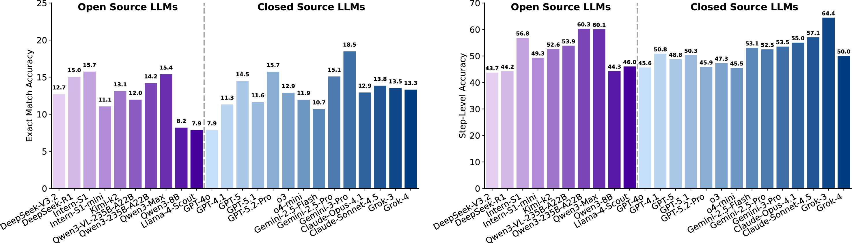
Grok-3 SLA substantially exceeds EM across nearly all systems. Multiple systems, including several agents-achieve SLA above 50%, with the best around 65%. This disparity suggests that models frequently produce partially correct or locally consistent reasoning steps but struggle to maintain coherence and correctness across the full reasoning chain. Such behavior underscores the intrinsic difficulty of end-to-end scientific reasoning and the importance of step-wise decomposition for improving task success.

Newer large-scale LLMs do not universally outperform predecessor models. For example, Grok-4 exhibits lower EM and SLA than Grok-3 on this benchmark, suggesting that large-scale training may introduce regressions or reduce retention of specialized scientific knowledge. These results collectively Question: The experimental methodology for studying chaotic hysteresis in Chua’s circuit is employs a precision Chua’s circuit setup with calibrated instrumentation to investigate chaotic hysteresis through step-by-step DC voltage variation and frequency-dependent triangular wave analysis, quantifying hysteresis loops and identifying critical frequency thresholds via phase space trajectory monitoring and time series bifurcation analysis. In the Chua circuit experiment, what are the calculated time constants (in μs) for the RC networks formed by a 10.2 nF capacitor C1 and the equivalent resistance, the peak-to-peak voltage (in V) range of the hysteresis loop at 0.01 Hz driving frequency, and the critical frequency (in Hz) where chaotic behavior ceases? Output the results in two decimal places, one decimal place, and integer format respectively, separated by commas.

/mnt/shared-storage-user/xuwanghan/projects/SuperSFE/SuperSFE/data/v7-3-深度搜索/ 物理/7_电路系统中的混沌行为/1/deep_research.json

Step 1: Find paper Experimental observation of chaotic hysteresis in Chua’s circuit driven by slow voltage forcing.

Step 2: Identify RC network components from experimental setup: C1=10.2 nF, R1=219Ω. Calculate time constant: τ=R1×C1=219×10.2×10-9=2.2338μs≈2.23μs.

Step 3: Voltage range determination: At 0.01 Hz triangular forcing, peak-to-peak voltage ΔV_T=3.2 V measured from hysteresis loop width in experimental phase portraits.

Step 4: Critical frequency identification: “For f>10Hz the hysteresis phenomenon practically disappears” confirmed through frequency sweep experiments showing ΔV_T reduction from 3.2V (0.01Hz) to 0V (10Hz).

Step 5: Validate measurement procedures: Hysteresis loops are measured by “changing DC voltage very slowly and step by step” while monitoring attractor transitions between single scroll and double scroll regimes.

Step 6: Confirm data analysis techniques: Phase portraits and time series analysis confirm chaotic behavior through “bifurcations and dynamic attractor folding”.

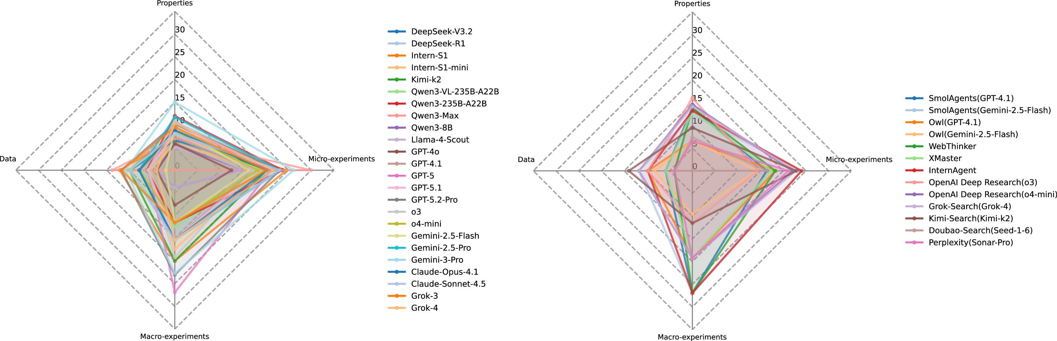
Step Most models exhibit substantially lower performance on the Data and Properties tasks, but somewhat better-though still modestly-on Micro-and Macro-experiment tasks. Based on the focus of each question, we categorize the tasks into four types: Data, Properties, Micro-experiments, and Macro-experiments (Table 1). Figure 14 summarizes the performance of LLMs and agents across these categories. Notably, performance across all four categories rarely exceeds 30% (with only a few Macro cases slightly above), underscoring the intrinsic difficulty of scientific deep research. This disparity can be attributed to the nature of the information required. Data-and property-related questions often rely on detailed numerical specifications or contextual descriptions scattered across disparate sources in the literature, demanding precise retrieval, cross-referencing, and aggregation. In contrast, Micro-and Macro-experiment tasks tend to provide more structured protocols or clearer experimental outcomes, enabling LLMs and agents to reason with fewer retrieval uncertainties.

In summary, the relatively stronger model performance on experiment-oriented tasks suggests that recent advances in LLM pretraining and instruction tuning have enhanced models’ abilities to process structured procedures and numerical patterns. Nevertheless, the consistently low scores across all categories indicate that contemporary LLMs, even when augmented with tool-based agents, remain far from mastering the breadth and depth of reasoning required for robust scientific deep research.

Figure 15 illustrates the evaluation pipeline for Idea Generation in SGI-Bench, and more experimental details can be found in the section 2.2.2. Table 6 shows the quantitative experimental results of idea generation, including effectiveness, novelty, detailedness, and feasibility. We could see that GPT-5 achieves the best average performance, and achieves the best performance in three aspects only excluding the feasibility. Moreover, across models, a clear pattern emerges: Novelty is generally high, especially among closed-source systems (e.g., o3 73.74, GPT-5 76.08). This indicates that modern LLMs possess a robust capacity for generating conceptually novel scientific ideas. Such behavior aligns with the growing empirical use of LLMs as inspiration engines for scientific hypothesis generation and exploratory research.

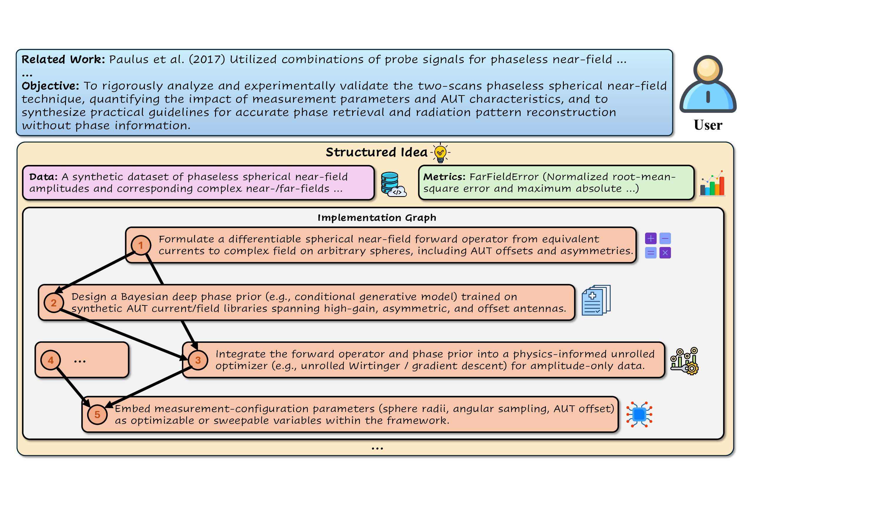
To rigorously analyze and experimentally validate the two-scans phaseless spherical near-field technique, quantifying the impact of measurement parameters and AUT characteristics, and to synthesize practical guidelines for accurate phase retrieval and radiation pattern reconstruction without phase information.

Formulate a differentiable spherical near-field forward operator from equivalent currents to complex field on arbitrary spheres, including AUT offsets and asymmetries.

1

Integrate the forward operator and phase prior into a physics-informed unrolled optimizer (e.g., unrolled Wirtinger / gradient descent) for amplitude-only data.

Embed measurement-configuration parameters (sphere radii, angular sampling, AUT offset) as optimizable or sweepable variables within the framework.

Design a Bayesian deep phase prior (e.g., conditional generative model) trained on synthetic AUT current/field libraries spanning high-gain, asymmetric, and offset antennas. Mechanistically, this strength likely stems from their broad pretraining over heterogeneous scientific corpora, which enables them to recombine distant concepts across domains, as well as their ability to internalize high-level research patterns (problem-method-evaluation triples

Experiments form the critical bridge between idea generation and scientific reasoning, providing the most direct avenue for validating hypotheses and uncovering new phenomena. Within SGI-Bench, we evaluate two complementary forms of experiments: dry experiments, which involve computational analyses or simulations, and wet experiments, which require laboratory procedures and operational planning. Across both categories, current AI models exhibit substantial limitations, revealing a persistent gap between linguistic fluency and experimentally actionable competence.

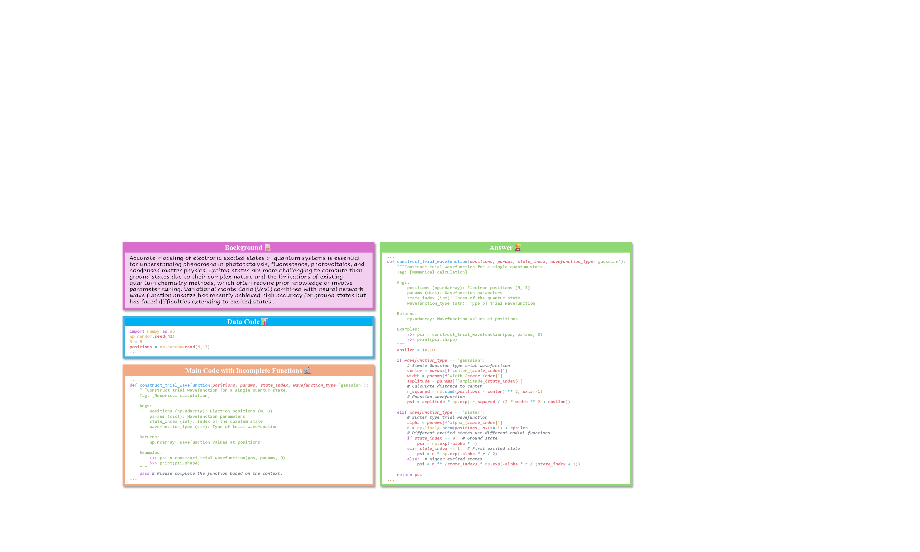
Accurate modeling of electronic excited states in quantum systems is essential for understanding phenomena in photocatalysis, fluorescence, photovoltaics, and condensed matter physics. Excited states are more challenging to compute than ground states due to their complex nature and the limitations of existing quantum chemistry methods, which often require prior knowledge or involve parameter tuning. Variational Monte Carlo (VMC) combined with neural network wave function ansatze has recently achieved high accuracy for ground states but has faced difficulties extending to excited states…

As introduced in Section 2.1.3, each dry experiment contains three components: a description of scientific background, a complete data-construction script, and an analysis script with masked functions. The model must infer and complete these missing functions using contextual understanding. For fairness and structural clarity, function headers, including names, signatures, and functional descriptions, are preserved, as shown in Figure 16. This setup isolates the model’s ability to infer algorithmic logic rather than boilerplate structure. Table 7 summarizes three metrics defined in Section 2.2.3: PassAll@k, Average Execution Time (AET), and Smooth Execution Rate (SER). Here, PassAll@k denotes passing at least 𝑘 out of five unit tests per problem. Under the lenient criterion (𝑘=1), the best models achieve a PassAll@1 score of 42.07%, whereas the strictest requirement (𝑘=5) reduces performance to 36.64%. These results underscore that scientific code completion remains a significant bottleneck, even for frontier LLMs. Notably, closed-source models generally achieve higher PassAll@k than leading open-source models, though the advantage is modest and distributions overlap, suggesting that scientific code synthesis in dry experiments remains underdeveloped across architectures.

High execution rates do not guarantee correctness. The SER metric captures whether the generated code executes without error, independent of correctness. While many top models achieve high SER values (>90%), performance varies widely across systems; several models are substantially below this threshold (e.g., Gemini-2.5-Flash/Pro, Qwen3-8B, Llama-4-Scout, GPT-5, GPT-4o), indicating nontrivial robustness gaps. This suggests that basic structural and API-level reasoning has matured for some models; however, the persistent gap between SER and accuracy metrics highlights that structural validity is far easier than algorithmic correctness in scientific contexts.

Numerical and simulation functions are the most challenging. Figure 17 breaks down PassAll@5 across functional types. Models perform relatively well on Data Processing and Predictive Modeling, where multiple valid implementations exist and errors are less amplified. In contrast, Numerical Calculation and simulation-oriented functions prove substantially more difficult. These tasks typically require precise numerical stability, accurate discretization, or careful handling of domain-specific Model PassAll@5(%)↑ PassAll@3(%)↑ PassAll@1(%)↑ AET(s)↓ SER(%)↑ constraints, all of which amplify small reasoning inconsistencies. This pattern reveals a striking asymmetry: models exhibit reasonable flexibility in tasks with diverse valid outputs but struggle with tasks requiring exact numerical fidelity.

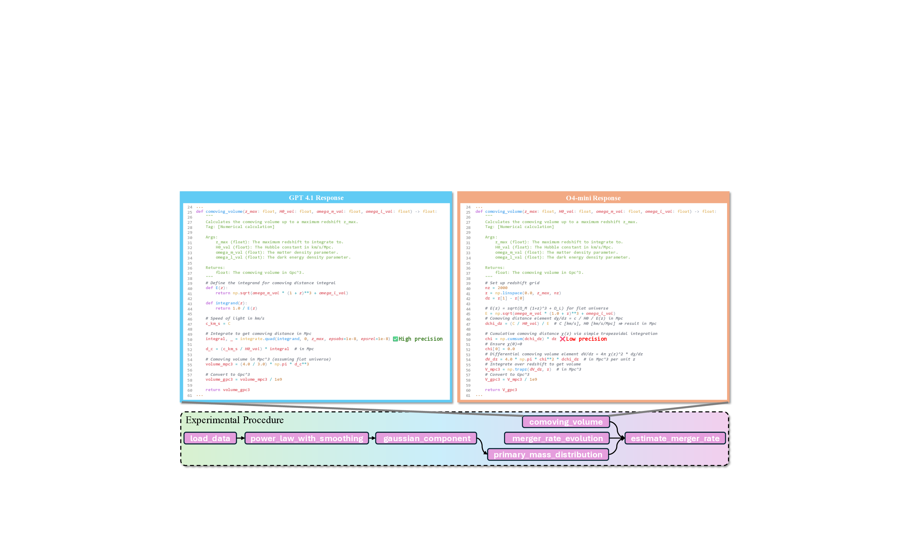
Methodological choices critically affect outcomes. The case shown in Figure 18 illustrates this issue in an astronomical dry experiment involving the computation of gravitational-wave observables from LIGO/Virgo-like detectors. The o4-mini model employs a naïve numerical integration via np.cumsum, effectively using a forward Euler approximation for

which introduces substantial cumulative error when the discretization is coarse. In contrast, GPT-4.1 correctly adopts scipy.integrate.quad, leveraging adaptive integration schemes that preserve numerical precision. Because errors in 𝜒(𝑧) propagate directly to the comoving volume element

the flawed integration strategy in o4-mini leads to a significant deviation in the final volume estimate 𝑉 Gpc 3 . This example highlights a broader challenge: LLMs often fail to capture the numerical sensitivity and methodological nuance essential for scientific computation.

Overall, these findings reveal that while current models can generate syntactically valid code with high reliability, their deeper limitations stem from (i) incomplete numerical reasoning, (ii) superficial understanding of scientific algorithms, and (iii) the inability to select appropriate computational strategies under domain constraints. AI-assisted scientific experimentation thus remains a demanding frontier, requiring future models to incorporate domain-aware numerical reasoning, fine-grained algorithmic priors, and training signals beyond natural-language supervision.

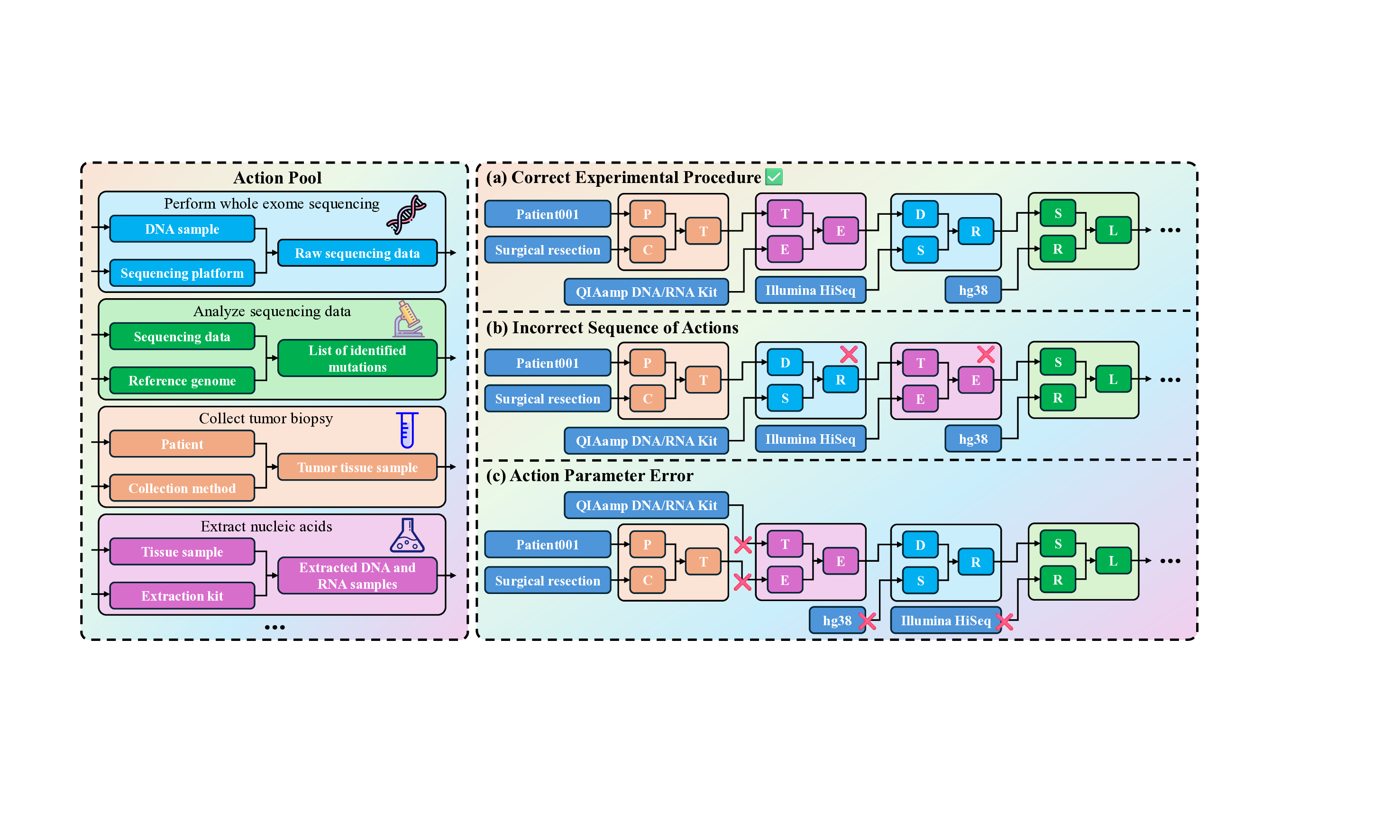
For wet experiments, we provide models with an action pool containing standardized experimental operations and detailed descriptions. Given the experimental context, the model is required to synthesize a complete workflow, including both the selection and ordering of actions as well as all associated parameters (Figure 19). As illustrated in the figure, the model outputs typically exhibit two major categories of errors: (i) incorrect ordering of experimental steps and (ii) inaccurate or inconsistent parameter specification.

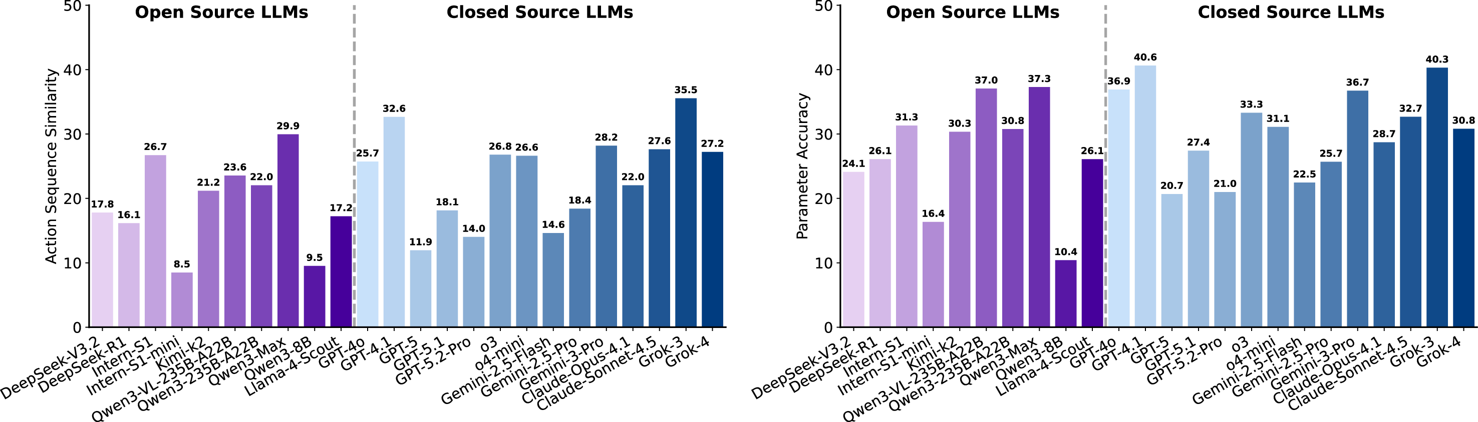
Collect tumor biopsy Wet experiments reasoning remains brittle. Figure 20 summarizes performance in terms of sequence similarity (SS) and parameter accuracy (PA). For SS, closed-source models in general achieve higher scores than open-source ones (with the best closed-source model around 35.5 versus the best open-source below 30), yet SS remains uniformly low across all systems. In contrast, PA exhibits a mixed pattern: although the top result is obtained by a closed-source model (around 40.6), several open-source models are competitive, and some closed-source models drop markedly (e.g., near 20.7). PA appears slightly more optimistic also since permutation-equivalent parameter groups are treated as identical (e.g., ⟨action 1⟩(𝐵, 𝐶) and ⟨action 1⟩(𝑋, 𝑌 ) are identical when 𝐵=𝑋 and 𝐶=𝑌 ), but both families still achieve only modest scores. Across outputs, errors recur in three patterns: insertion of unnecessary steps, omission of essential steps, and incorrect ordering of valid steps.

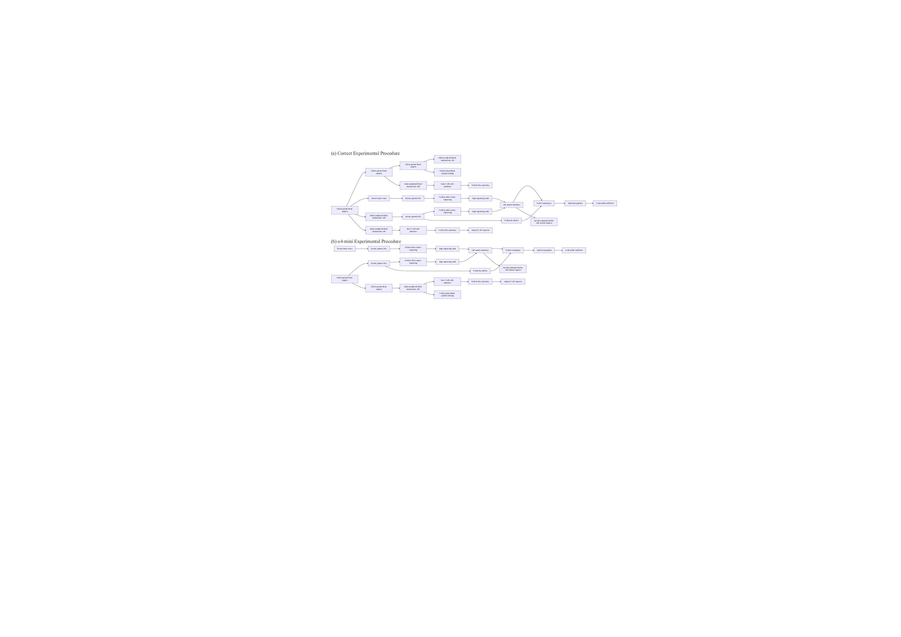
Temporal and branch-aware planning is often broken. Figure 21 presents an experiment examining how tumor mutational burden and neoantigen load influence the efficacy of anti-PD-1 immunotherapy in non-small cell lung cancer. The ground-truth workflow (Figure 21 a) features a deeply branched structure with precisely coordinated timing and sample-handling procedures. In contrast, the workflow generated by o4-mini is substantially simplified and deviates from several core principles of experimental design. First, the model collapses longitudinal sampling into a single blood draw and does not distinguish time windows, precluding any meaningful reconstruction of T-cell dynamics. Second, PBMC isolation is executed only once rather than per time point, causing misalignment with downstream staining and flow cytometry. Functional assays (e.g., intracellular cytokine staining) are performed on a single PBMC aliquot without branching by time point or antigenic stimulation, and flow cytometry is likewise conducted only once, failing to capture temporal variation. Finally, the blood-sample branch conflates genomic and immunophenotyping workflows: “Extract genomic DNA” is executed in parallel with PBMC isolation and downstream immunology, leading to duplicated and cross-purpose use of peripheral blood. These design flaws mirror the low sequence similarity and only moderate parameter accuracy observed in Figure 20, underscoring failures in temporal coordination, branchaware planning, and sample bookkeeping.

Overall, the deviations highlight a critical limitation of current AI models: while they can enumerate plausible wet experiment actions, they struggle to construct experimentally valid, temporally consistent, and branch-aware protocols. These limitations point to fundamental gaps in reasoning about experimental constraints, biological timing, and multi-sample coordination-elements essential for real-world scientific experimentation.

Experimental Reasoning evaluates the ability of multimodal LLMs to interpret experimental observations, integrate heterogeneous scientific evidence, and refine testable hypotheses. As illustrated in Figure 22, the visual inputs span five representative modalities in scientific practice-process diagrams, data visualizations, natural observations, numerical simulations, and laboratory experiments-reflecting the diversity of multimodal information that underpins real-world scientific inquiry.

In this task, models are provided with several images accompanied by a question and must select the correct answer from at least ten candidates (Figure 23). Solving these problems requires multistep inferential reasoning: identifying relevant variables, synthesizing multimodal cues, evaluating competing hypotheses, and ultimately validating consistency across the provided evidence. We therefore evaluate model performance using both Multi-choice Accuracy and Reasoning Validity, the latter assessing whether the model’s explanation follows logically from the scientific evidence.

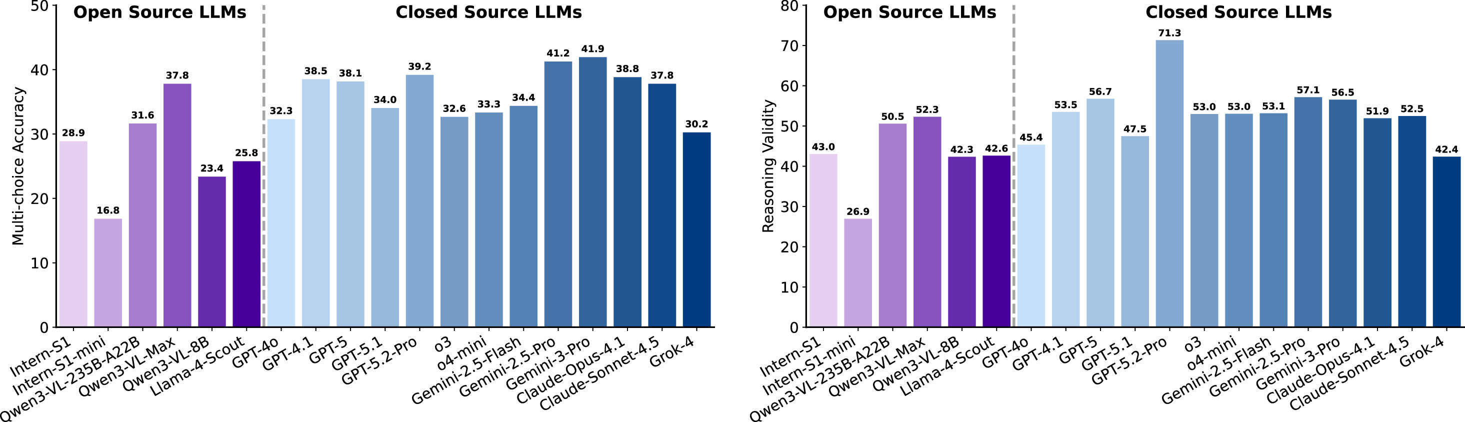
Reasoning validity often exceeds answer accuracy. As shown in Figure 24, closed-source LLMs generally outperform open-source counterparts on both metrics, with the best closed-source models achieving higher MCA (e.g., up to 41.9) and RV (e.g., up to 71.3) than the best open-source models (MCA 37.8, RV 52.3). However, several open-source models remain competitive with or exceed some closed-source systems in specific metrics (e.g., Qwen3-VL-235B-A22B RV 50.5 > GPT-4o RV 45.4), indicating nontrivial overlap. Most models score higher in Reasoning Validity than in Multi-choice Accuracy, suggesting that even when the final choice is incorrect, explanations often preserve partial logical coherence. Variance is moderate-particularly among closed-source models-while only a few models (e.g., Intern-S1-mini) show noticeably lower performance, pointing to the importance of scale for robust multimodal scientific reasoning.

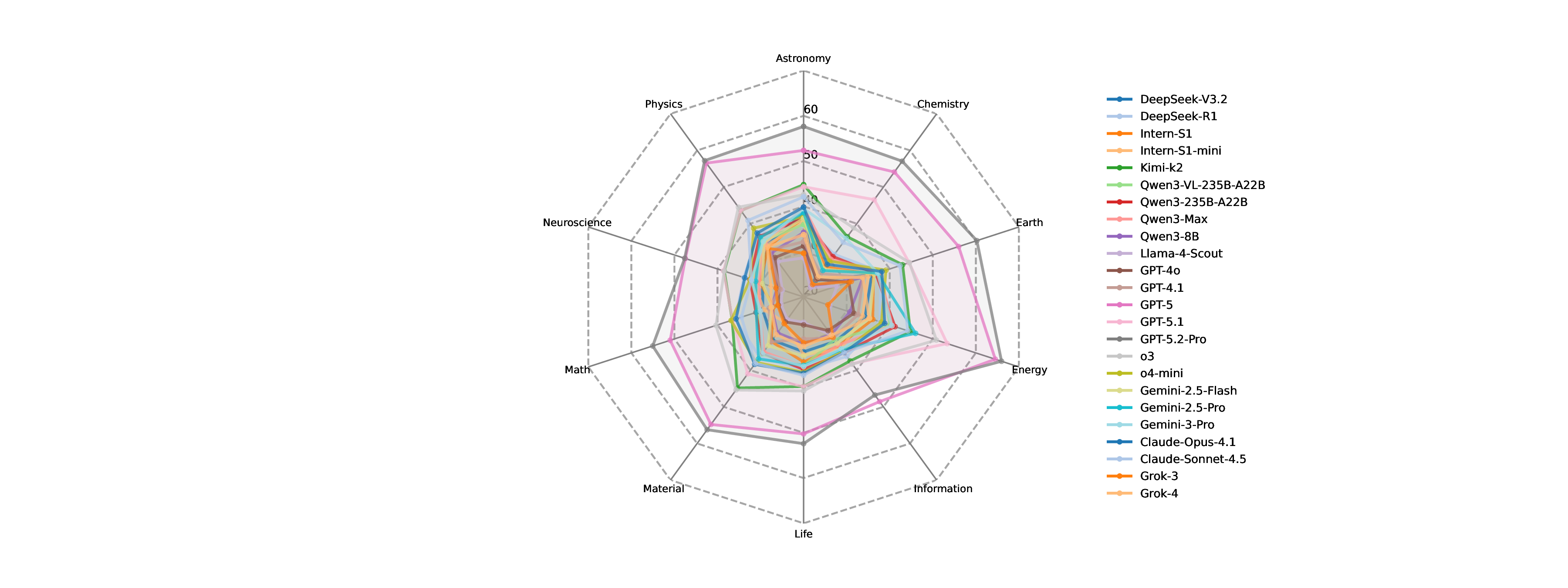
Comparative reasoning is the most challenging across domains. To further dissect these capabilities, we analyze performance across reasoning types and disciplinary domains (Figure 25). From the perspective of reasoning categories, including signal perception, attribute understanding, comparative reasoning, and causal reasoning, LLMs perform consistently well in causal reasoning and perceptual recognition. In contrast, comparative reasoning emerges as a persistent weakness. This indicates that models struggle when required to contrast subtle quantitative or qualitative differences, a cognitive operation fundamental to scientific evaluation and hypothesis discrimination. When examining performance across 10 scientific disciplines, an intriguing pattern emerges. Models achieve their highest accuracy in astronomy, followed by chemistry, energy science, and neuroscience. These domains often feature structured visual patterns or canonical experimental setups, which may align well with LLMs’ prior training data. Conversely, performance declines substantially in materials science, life sciences, and Earth sciences, where visual cues are more heterogeneous, context-dependent, or experimentally nuanced. This divergence suggests that domain-specific complexity and representation diversity strongly influence multimodal reasoning performance. Overall, these findings reveal that while current LLMs demonstrate encouraging abilities in integrating scientific evidence and conducting basic causal analyses, they still fall short in tasks requiring precise discrimination, cross-sample comparison, and nuanced interpretation of domain-specific observations. The relatively narrow performance gap among leading models underscores that scale alone is insufficient; advancing experimental reasoning will require improved multimodal grounding, finer-grained visual understanding, and training paradigms explicitly aligned with scientific inquiry.

Large Language Models (LLMs) have demonstrated remarkable capabilities in reasoning and problemsolving, primarily driven by supervised fine-tuning and reinforcement learning on extensive labeled datasets. However, applying these models to the frontier of scientific discovery, particularly in the task of scientific idea generation, presents a fundamental challenge: the inherent absence of ground truth. Unlike closed-domain tasks such as mathematical reasoning or code generation, where solutions can be verified against a correct answer, the generation of novel research ideas is an open-ended problem with no pre-existing “gold standard” labels. This limitation renders traditional offline training pipelines insufficient for adapting to dynamic and unexplored scientific territories.

To address this, we adopt the paradigm of Test-Time Reinforcement Learning (TTRL) [20]. This framework enables models to self-evolve on unlabeled test data by optimizing policies against rule-based rewards derived from the model’s own outputs or environmental feedback. Distinct from the original implementation [20], which primarily leveraged consensus-based consistency as a reward mechanism for logical reasoning tasks, we establish novelty as our core optimization objective in the current context. Consequently, we introduce a TTRL framework where the reward signal is constructed based on the dissimilarity between generated ideas and retrieved related works, guiding the model to actively explore the solution space and maximize innovation at test time.

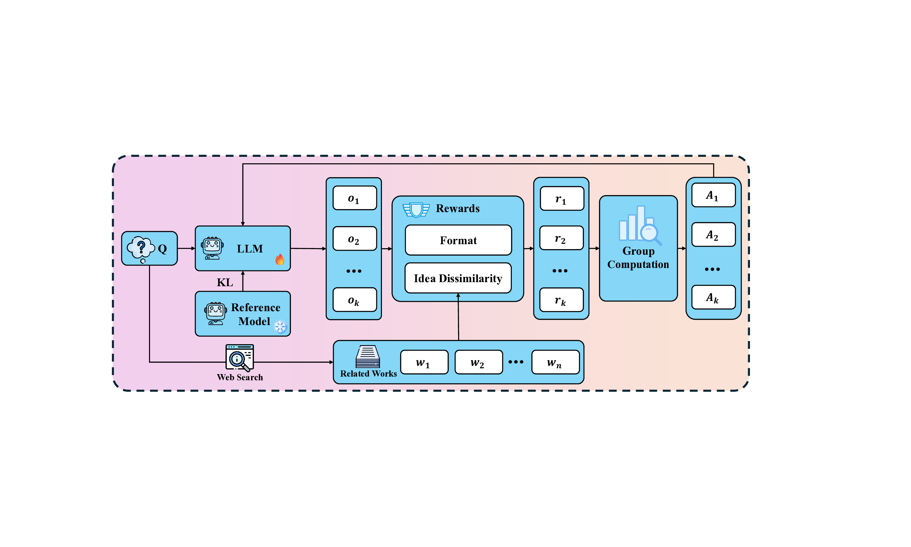
To address the absence of ground truth in scientific idea generation, we propose a generalizable reward mechanism based on online retrieval. Instead of relying on static labels, we utilize real-time search to fetch existing related works, serving as a dynamic baseline for comparison. This approach enables us to quantify novelty as the semantic dissimilarity between the model’s output and the retrieved context, effectively converting an open-ended exploration problem into a measurable optimization task. The overall training framework is illustrated in Figure 26.

We employ Group Relative Policy Optimization (GRPO) [1] as our training backbone. For a given query 𝑄, the policy model 𝜋 𝜃 generates a group of 𝑘 outputs {𝑜 1 , . . . , 𝑜 𝑘 }. The optimization is guided by a composite reward function, defined as the unweighted sum of a format constraint and a novelty metric (labeled as Idea Dissimilarity in Figure 26):

where W = {𝑤 1 , . . . , 𝑤 𝑛 } denotes the set of related works obtained via online search.

To guarantee interpretable reasoning, we enforce a strict XML structure.

The model must encapsulate its chain of thought within … and the final proposal within …. The format reward is binary:

Novelty Reward (𝑅 novelty ). We quantify novelty by measuring the vector space dissimilarity between the generated idea and the retrieved literature. Let e idea be the embedding of the generated answer, and {e 𝑤 𝑗 } 𝑛 𝑗=1 be the embeddings of 𝑛 retrieved papers (denoted as 𝑤 1 , . . . , 𝑤 𝑛 in the figure). We compute the average cosine similarity 𝑆 avg :

An innovation score 𝑆 inn ∈ [0, 10] is then derived to reward divergence:

Using a gating threshold 𝜏 = 5, the final novelty reward is defined as:

This mechanism incentivizes the model to produce ideas that are semantically distinct from existing work.

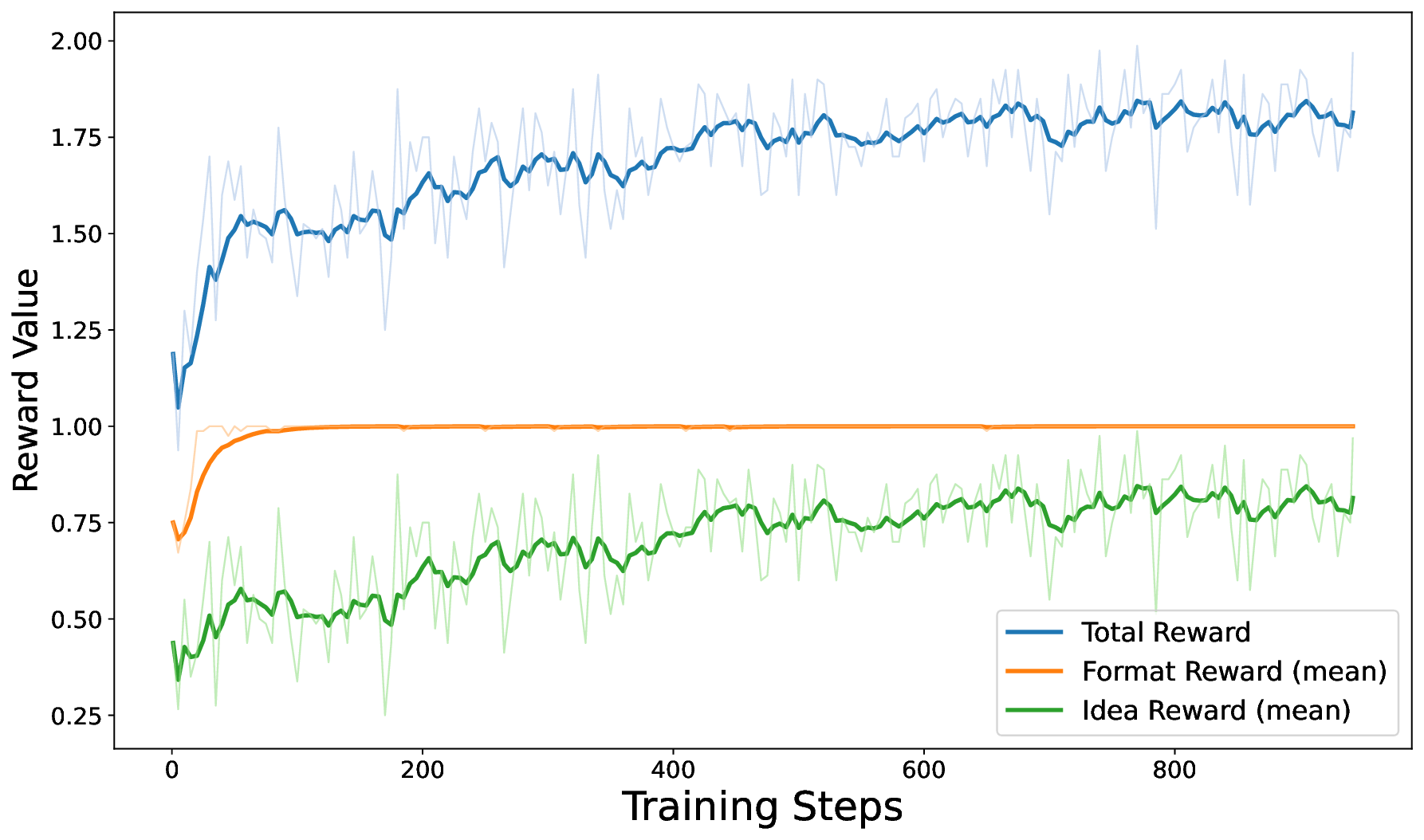
We employ Qwen3-8B as the base model, trained using the GRPO algorithm within the ms-swift [77] framework. To facilitate diverse exploration, we utilize a high sampling temperature. Key hyperparameters are detailed in Table 8. Figure 27 | TTRL Training Dynamics: Format reward saturates quickly, followed by steady growth in idea novelty.

The training dynamics of our TTRL framework are illustrated in Figure 27. The curves demonstrate a clear two-phase optimization process. Initially, the Format Reward (orange line) rises rapidly and saturates near 1.0 within the first few steps, indicating that the model quickly adapts to the rigid XML structural constraints ( and tags). Once the format is stabilized, the Idea Reward also starts to rise (green line). Despite the inherent difficulty of the task, the Idea Reward exhibits a consistent upward trend throughout the training steps, driving the total reward (blue line) to converge at a higher value.

Quantitatively, this self-evolution process yields a significant improvement in the quality of generated ideas. The average novelty score of the model’s outputs increased from a baseline of 49.36 to 62.06.

It is important to emphasize that this performance gain was achieved entirely without ground-truth labels. The model improved solely by leveraging the online retrieval feedback loop, validating the hypothesis that LLMs can self-improve on open-ended scientific discovery tasks through test-time reinforcement learning.

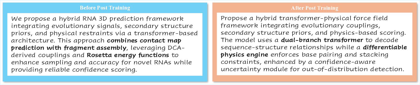
To visually demonstrate the impact of TTRL on scientific idea generation, we present a comparative case study in Figure 28. The task requires the model to propose a novel framework for RNA 3D structure prediction.

We propose a hybrid RNA 3D prediction framework integrating evolutionary signals, secondary structure priors, and physical restraints via a transformer-based architecture. This approach combines contact map prediction with fragment assembly, leveraging DCAderived couplings and Rosetta energy functions to enhance sampling and accuracy for novel RNAs while providing reliable confidence scoring.

Propose a hybrid transformer-physical force field framework integrating evolutionary couplings, secondary structure priors, and physics-based scoring.

The model uses a dual-branch transformer to decode sequence-structure relationships while a differentiable physics engine enforces base pairing and stacking constraints, enhanced by a confidence-aware uncertainty module for out-of-distribution detection.

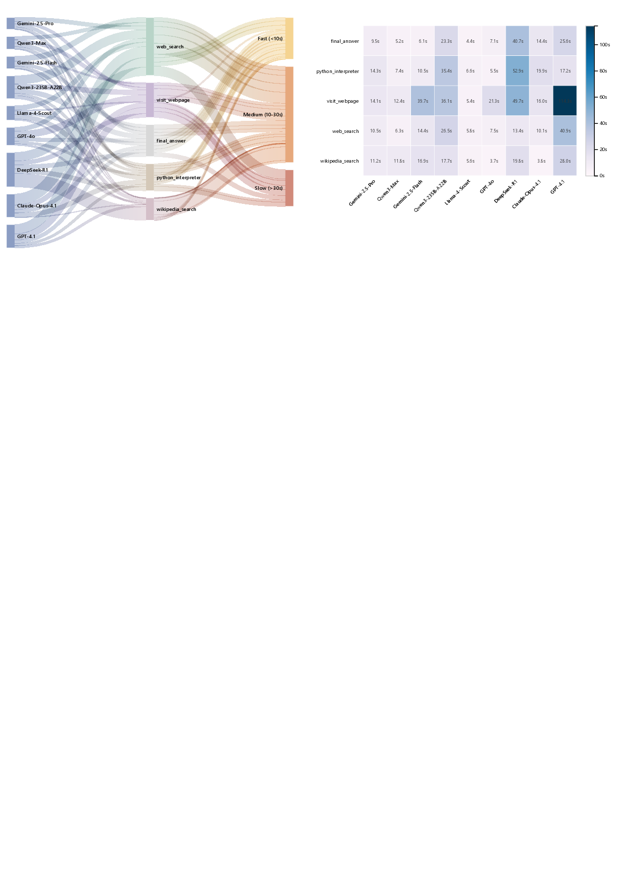
Tool-Integrated Reasoning (TIR) in real tasks unfolds as a dynamic, opportunistic process rather than a fixed linear chain [78]. As shown in Figure 29 (left), the model-to-tool flow concentrates heavily on retrieval actions: web_search is the most frequently invoked tool with 539 calls (33.98% of all), followed by visit_webpage (385, 24.27%), final_answer (358, 22.57%), python_interpreter (200, 12.61%), and wikipedia_search (104, 6.56%). This distribution indicates that an external “retrieve-then-browse” loop remains the dominant path for contemporary agentic systems, reflecting persistent limits in time-sensitive and domain-specific knowledge available to base LLMs. Importantly, models differ in how efficiently they traverse this loop: for example, GPT-4.1 issues large volumes of web_search (168) and visit_webpage (110) that frequently land in slow tiers, whereas Qwen3-Max completes comparable coverage with far fewer retrieval and browsing steps (61 and 59, respectively). Practically, this pattern implies that reducing redundant retrieval iterations-via better query formulation and higher-quality extraction on the first pass-has immediate leverage on end-to-end latency, often exceeding gains from marginal improvements to raw model inference.

Latency variation is predominantly tool-dependent, as visualized in Figure 29 (right). The primary bottleneck is visit_webpage, whose cross-model latency spans from 5.37s (Llama-4-Scout) to 114.29s (GPT-4.1), a 21.28× spread. This reflects the intrinsic cost of browser-level execution-network I/O, DOM parsing, and event replay-rather than LLM reasoning alone. In contrast, more atomic operations such as wikipedia_search still exhibit a substantial 7.59× spread (3.69-28.03s), underscoring that I/O pathways and parsing routines meaningfully shape end-to-end time even for ostensibly simple tools. These observations suggest a design priority: engineering optimizations in the retrieval-and-browsing pipeline (e.g., smarter caching, incremental browsing, selective content extraction) will reduce both long-tail latencies and overall wall-clock time more reliably than tuning model-only parameters.

The python_interpreter tool exhibits a 9.65× cross-model range (5.48-52.94s), indicating that measurements capture the full “reason-execute-debug-repair” loop rather than a single code run. The slowest average arises for DeepSeek-R1 (52.94s), consistent with more frequent multi-step error analysis and correction; the fastest is GPT-4o (5.48s), reflecting a low-latency, near single-shot execution path. This divergence reveals a strategic trade-off: systems optimized for first-attempt correctness minimize tool time but may forgo deeper self-correction, whereas systems favoring iterative refinement accrue longer tool-side latency while potentially achieving more robust final solutions.

In practice, aligning tool routing, retry policy, and verification depth with a model’s characteristic behavior can reduce wasted cycles and sharpen the latency-quality frontier.

SGIEvalAgent interprets the user’s evaluation intent and turns it into a rubric that can be applied consistently across the selected idea-generation questions. In the case shown in Figure 30, the user asks to compare models on “rigor” in cross-disciplinary idea generation. The system formalizes Rigor (scientific strictness) for idea proposals so that it reflects how scientists judge whether a plan is internally coherent, well grounded, and practically verifiable.

The rubric expresses six aspects in prose rather than checklists. First, it checks logical self-consistency and completeness of the pipeline from problem to hypothesis, method, metrics, and expected results. Second, it requires theory and literature grounding that either correctly inherits prior work or responsibly challenges it with evidence. Third, it demands precise and verifiable problem definitions that state goals, constraints, evaluation metrics, and success conditions. Fourth, it looks for deep fit with the research background and correct, discipline-aligned terminology. Fifth, it evaluates methodological soundness and reproducibility through executable steps, a clear I/O loop, and explicit rationale for key design choices. Sixth, it considers risk awareness and scientific criticism by articulating assumptions, potential failure modes, bias sources, and avoiding over-confident conclusions. Major deductions apply when the reasoning chain is missing, key assumptions are unstated, terminology is misused, metrics are vague or non-verifiable, or inheritance from background knowledge is misaligned.

Scores are produced on a 0-10 scale for each aspect and aggregated with default equal weights I want to know which model has the best rigor in idea generation across science disciplines.

Selected idea-generation questions across Physics, Chemistry, Biology, and seven other disciplines from SGI-Bench to reflect cross-disciplinary scientific ideation.

User-customized metric: Rigor (scientific strictness).

Running inference and scoring…

We evaluate models on the user-defined Rigor metric for idea generation. Observations from the chart: 1. Closed-source LLMs generally achieve higher rigor; top performers cluster around the GPT-5/o3/o4-mini families. into a single rigor score; the result is linearly mapped to a 0-100 axis for visualization without changing rank order. The evaluation agent generates textual rationales that cite reference answers and problem context so that decisions are transparent and reproducible. Customized metrics are reported alongside SGI-Bench’s predefined task metrics rather than replacing them, preserving standardized comparability while highlighting the user’s domain-specific focus.

The reporting agent summarizes the customized metric and the evaluation outputs into a concise narrative with figures. In Figure 30, the report contrasts open-source and closed-source systems on the user-defined rigor metric for idea generation and highlights what the scores mean in practice.

The core takeaway is straightforward: closed-source models generally exhibit higher rigor under this rubric, intra-family iterations capture measurable gains, and leading open-source models show notable progress that narrows the gap. Higher rigor reflects more structured, well-grounded, and verifiable research plans rather than merely fluent narratives. The report therefore gives users a clear, scientist-aligned comparison they can directly use for model selection and iteration in research workflows.

Grounded in our operational definition of SGI and instantiated through SGI-Bench, the evaluation results reveal a consistent message: contemporary LLMs and agentic systems exhibit localized scientific cognition and segmented scientific reasoning They may solve isolated sub-problems, but fail to robustly close the iterative loop spanning Deliberation, Conception, Action, and Perception. Below we summarize the main limitations across tasks and disciplines, connect them with our TTRL and tool-integrated reasoning analyses, and outline concrete future directions. 12, Figure 13). This indicates that current models still fail to produce verifiable final scientific claims under multi-source evidence integration.

A notable gap exists between SLA and EM. SLA is substantially higher for nearly all systems, with several agentic systems reaching ≈50% SLA (Figure 13), while EM remains low. This disparity shows that models often produce locally correct steps but cannot maintain global coherence across long reasoning chains. The failure mode is therefore not mere knowledge absence, but reasoning trajectory collapse under long-horizon scientific inference.

At a finer granularity, Deep Research tasks involving Data and Properties are the weakest: performance on these categories is substantially below that of Microand Macro-experiment questions, with all four categories rarely exceeding 30% accuracy (Figure 14). This aligns with the task design: data/property questions require retrieving dispersed numerical details across heterogeneous papers, while experiment-oriented questions provide more structured evidence. The results thus expose a core SGI bottleneck: meta-analytic retrieval + numerical aggregation over scattered literature. Action: Experimental execution is limited by numerical and procedural rigor. For Dry Experiments, accuracy is measured by PassAll@k. Even under the most lenient setting, the best PassAll@1 is only 42.07% (Claude-Sonnet-4.5), and under the strictest criterion, the best PassAll@5 rises to merely 36.64% (Gemini-3-Pro) (Table 7). The spread between PassAll@1 and PassAll@5 (e.g., 42.07→35.79

for Claude-Sonnet-4.5, 41.98→36.64 for Gemini-3-Pro) indicates that models often nail partial logic but fail full scientific correctness.

Importantly, code executability is not the bottleneck: most frontier models achieve SER > 90% (e.g., GPT-5.1 96.53, Gemini-3-Pro 98.85), while accuracy remains low. This gap confirms a central limitation: syntactic fluency ≠ scientific computational reasoning. The per-function analysis further shows numerical-calculation and simulation functions as the major failure mode (Figure 17), consistent with the case study (Figure 18) where naive integration choices lead to cascading scientific errors.

For Wet Experiments, although Parameter Accuracy improves slightly under permutation-equivalence evaluation, Sequence Similarity remains uniformly low across both open and closed models (Figure 20). Models frequently insert redundant steps, omit critical actions, or misorder multi-branch protocols. The complex oncology workflow case (Figure 21) illustrates that models cannot reliably manage temporal design, branching logic, or multi-sample coordination. Thus, wet-lab action planning remains a profound gap toward embodied SGI.

Perception: Multimodal reasoning is improving, but comparison is a hard frontier. In Experimental Reasoning, closed-source models consistently outperform open-source ones (Figure 24). Across nearly all models, Reasoning Validity (RV) exceeds Multi-choice Accuracy (MCA), showing that models can often produce partially coherent narratives even when selecting the wrong option. This echoes the SLA-EM gap in Deep Research and suggests a general pattern: models are better at producing plausible local reasoning than globally correct scientific decisions.

Reasoning-type breakdown reveals that models perform relatively well on Signal Perception and Causal Reasoning, but Comparative Reasoning is persistently weakest (Figure 25). Scientific comparison requires subtle cross-sample discrimination and quantitative contrast-a cognitive operation central to scientist judgment but not yet robustly captured by current MLLMs. Discipline-wise, astronomy and chemistry are easier, while materials science, life science, and Earth science remain hardest (Figure 25), reflecting the mismatch between real scientific visual heterogeneity and training priors. 27) and qualitatively progresses from generic component assembly to structured innovation (Figure 28). These results suggest that SGI should be interpreted not merely as a static benchmark score, but as a capability that can evolve through test-time learning. Nevertheless, optimizing for novelty in isolation risks ungrounded or implausible ideas; combining novelty with rigor-or feasibility-based rewards is a crucial next step for reliable scientific ideation.

The retrieval pipeline is the true bottleneck for agentic SGI. Tool-Integrated Reasoning (TIR) analysis reveals that agent workflows are heavily dominated by retrieval operations: web_search accounts for 539 calls (33.98%), and visit_webpage for 385 calls (24.27%) (Figure 29). Latency is primarily tool-driven rather than model-driven; visit_webpage exhibits a 5.37s-114.29s range across models (a 21.28× spread). This indicates that many gains in SGI performance may stem from smarter tool routing, reduction of redundant retrievals, and higher-quality first-pass extraction, rather than simply scaling base LLMs. Analysis of the Python tool further highlights a trade-off between first-shot correctness and iterative self-repair, with a 9.65× cross-model latency range, underscoring the need for model-aware verification and retry policies in practical agentic workflows.

Our findings point to several high-leverage research directions:

(1) Meta-analytic reasoning with numerical robustness. Deep Research failures on Data/Properties and low EM despite high SLA call for methods that explicitly train evidence aggregation and numerical synthesis. Promising routes include retrieval-conditioned quantitative reasoning, uncertaintycalibrated aggregation over multiple sources, and verification-aware step planning that penalizes reasoning-chain drift.

(2) Planning-aware conception and structured supervision. To address uniformly low feasibility and sparse implementation detail in Idea Generation, adopt planning-aware constraints with structured supervision: require parameter-complete, dependency-consistent steps, prioritize feasibilityfocused rewards (availability checks, resource/cost estimates, reproducibility), and use lightweight tool checks during decoding to block or repair incomplete plans. This shifts fluent proposals into executable, testable designs under realistic scientific constraints.

(3) Scientific code training beyond syntax. Dry experiments show high SER but low PassAll@5 (Table 7), especially on numerical and simulation functions (Figure 17). Future work should emphasize numerical analysis priors, stability-aware loss, and algorithmic-choice training (e.g., recognizing when adaptive integration or stiffness solvers are required). Hybrid symbolic-numeric tool use (formal solvers + LLM reasoning) is another promising path.

(4) Branch-and time-aware wet-lab protocol reasoning. Uniformly low Sequence Similarity and qualitative failures on complex branching protocols (Figure 21) suggest a need for training signals that encode temporal sampling logic, branching decision rules, and multi-sample tracking. Action-pool grounding can be extended with stateful simulators or lab-graph verifiers, enabling models to learn procedural validity under physical constraints.

(5) Comparative multimodal scientific reasoning. Comparative reasoning is the hardest paradigm (Figure 25). Progress likely requires finer-grained visual grounding (e.g., numeric extraction from charts), cross-image alignment modules, and contrastive multimodal training that rewards precise discrimination rather than narrative plausibility. Discipline-specific multimodal curricula may reduce domain gaps in materials/Earth/life sciences.

(6) Test-time learning with multi-objective scientific rewards. TTRL improves novelty without labels, but novelty alone is insufficient for SGI. Future TTRL systems should optimize a portfolio of scientist-aligned rewards (novelty, rigor, feasibility, safety, and experimental cost), and incorporate retrieval trustworthiness and contradiction penalties to prevent spurious innovation.

(7) Efficient and reliable tool ecosystems for SGI agents. Given retrieval dominance and tool latency (Figure 29), engineering advances are essential: retrieval caching, selective browsing, structured extraction, and tool-aware planning policies can substantially improve SGI agents’ end-to-end quality-latency frontier.

Summary. SGI-Bench reveals that modern LLMs exhibit partial competencies in each SGI quadrant but lack integrated, numerically robust, and methodologically disciplined scientific cognition. Bridging this gap requires progress on long-horizon meta-analysis, executable planning, numerically faithful experimentation, branch-aware wet-lab reasoning, comparative multimodal inference, and dynamic test-time self-improvement-all supported by efficient and trustworthy tool ecosystems. These directions collectively chart a concrete path from fragmented scientific skills toward genuine Scientific General Intelligence.

Despite providing a structured framework for evaluating scientific capabilities across four workflow stages, the current version of SGI-Bench has several limitations:

(1) Partial coverage of real scientific workflows. The four stages in our benchmark function as probes for different components of scientific inquiry rather than a complete representation of real-world scientific practice. Many aspects of scientific work-such as integration across scientific disciplines and risk and safety assessment [79]-remain outside our current scope.

(2) Scientific Deep Research currently emphasizes literature-inquiry-centric tasks. Deep Research spans activities such as literature inquiry [32], report-style reasoning [33], and related scientific analyses. In this benchmark, we focus on the literature-inquiry-centric subset, as identifying, interpreting, and integrating existing scientific knowledge is a foundational prerequisite for methodological design and experimental planning. This focus enables standardized, reproducible, and scalable evaluation while still probing a core component of real scientific workflows. More open-form variants-such as argumentative evidence synthesis or report generation-are also important but require substantial expert-based scoring, and are therefore reserved for future versions.

(3) Idea Generation evaluation focuses on methodology design. Fully open-ended hypothesis generation involves substantial conceptual freedom and requires extensive expert adjudication to achieve reliable judgments. Due to practical constraints, our current evaluation focuses on the methoddesign component of scientific ideas [34,35,36]. Future extensions may incorporate hypothesis-level evaluation through a combination of arena-style model comparisons and expert review.

(4) Limited code and action space coverage. Dry Experiment tasks currently support only Python [42], lacking adaptation to other programming languages and computational paradigms. The action space for Wet Experiments is an early-stage abstraction; scaling it requires constructing a large, standardized library of atomic actions grounded in real laboratory protocols [43].

(5) Experimental reasoning in enclosed spaces. We employ a multiple-choice design to ensure objective, automatable evaluation [45]. While practical, this structure constrains the model’s ability to express diverse reasoning paths and limits assessment of open-form scientific explanations.

(6) Partial coverage of deductive and inductive paradigms of scientific discovery. Scientific discovery is commonly understood to follow two broad paradigms: deduction and induction [80,81]. Deductive processes begin from prior knowledge or theoretical propositions and proceed through reasoning to experimental verification. Inductive processes, in contrast, originate from new observational data or unexpected empirical phenomena and generalize toward broader patterns or hypotheses.

The PIM-grounded [10,11] workflow in this version of SGI-Bench primarily reflects the deductive paradigm, as tasks begin with literature-based information and guide models toward reasoning and experiment planning. Inductive scientific discovery-which relies on data-driven pattern formation and hypothesis emergence-remains outside the scope of the current benchmark and represents an important direction for future expansion.

With the rapid advancement of Large Language Models (LLMs) and multi-agent systems in scientific reasoning, numerous datasets have emerged to evaluate their capabilities across various scientific domains.

A significant portion of existing benchmarks focuses on specific disciplines. In the physical sciences, PhyBench [82] examines multi-step reasoning and expression capabilities through original physics problems, while PHYX [83] focuses on real-world scenarios to assess physical reasoning and visual understanding. Additionally, PHYSICS [84] tests models using open-ended, university-level problems.To further address multimodal challenges, PhysUniBench [85] introduces a large-scale benchmark for undergraduate-level physics, specifically targeting the interpretation of physical diagrams and multi-step reasoning. In chemistry, ChemBench [86] provides domain-specific data for systematic evaluation, whereas ChemMLLM [87] extends this to multimodal assessment. More granular tasks are covered by benchmarks like ChemSafetyBench [88] and SpectrumWorld [89]. In life sciences, benchmarks range from the molecular level, such as DeepSEA [90] and GenomicsLong-Range [91], to healthcare applications like BioASQ [92] and VQA-RAD [93], as well as agricultural applications like SeedBench [94] and neuroscience with BrainBench [95]. For earth sciences, OmniEarth-Bench [96] covers a comprehensive range of fields with cross-domain tasks, EarthSE [97] builds a multi-level evaluation system from foundational to open-ended exploration, and MSEarth [98] utilizes high-quality scientific publications for graduate-level assessment. In remote sensing, GeoBench [99] and XLRS-Bench [100] evaluate perception and reasoning on high-resolution imagery. Furthermore, specialized benchmarks exist for other fields, including material science (MoleculeNet [101]), astronomy (AstroLLaMA and AstroMLab [102]), ocean science (OceanBench [103]), and climate science (ClimaQA [104]). These works primarily target deep evaluation within isolated disciplines. While benchmarks like ATLAS [105] have expanded to cover cross-disciplinary fields with high-difficulty standards, its evaluation specifically focuses on distinguishing frontier models through complex scientific reasoning and logical application tasks rather than the entire process of scientific discovery.

Concurrently, other benchmarks focus on cross-disciplinary comprehensive capabilities, though their evaluation focus is often distributed across specific stages of the scientific discovery pipeline. Regarding idea generation at the research inception stage, MOOSE-Chem2 [37] evaluates models through a win/tie/lose comparison framework that scores generated hypotheses against reference answers using multiple independent judges. AI Idea Bench 2025 [106] evaluates the novelty of agent-generated ideas using a dataset derived from top-tier conference papers. In the core layer of knowledge processing and analysis, some benchmarks focus on literature comprehension. For instance, SciAssess [107] decomposes analysis into memory, understanding, and reasoning layers. Others, like SFE [45], introduce a cognitive framework to dissect multimodal performance on raw scientific data. Complementing these, SciReasoner [108] targets the alignment of natural language with heterogeneous scientific representations. Recent works also evaluate comprehensive academic survey capabilities:

DeepResearch Bench [33] measures report quality and citation grounding, Manalyzer [109] focuses on mitigating hallucinations in automated meta-analysis, and Scientist-Bench [110] highlights the full workflow from review to paper generation. Additionally, SciArena [111] proposed an open platform that dynamically evaluates and ranks the performance of base models on scientific literature tasks by collecting pairwise comparison preferences from domain researchers, and DeepResearch Arena [112] utilizes seminar-grounded tasks to evaluate the orchestration of multi-stage research workflows, while AAAR-1.0 [113] focuses on evaluating the model’s ability as an AI-assisted research tool. In terms of planning and execution, evaluations often center on tool usage and coding. ToolBench [114] and ToolUniverse [115] explore API usage and standardization. In scientific coding, SciCode [42] and ScienceAgentBench [116] assess code generation within realistic workflows. At a macro level, MLE-bench [117] and TaskBench [118] evaluate general planning and project management via Kaggle competitions and task decomposition graphs. In addition, DISCOVERYWORLD [119] launched the first virtual environment for evaluating the ability of intelligent agents to perform a complete cycle of novel scientific discovery. However, it focuses on a gamified simulation environment, and its task scenarios and evaluation dimensions cannot fully reflect the complexity and high-level cognitive needs of real scientific research workflows. LLM-SRBench [120] , on the other hand, focuses only on the model’s ability to discover scientific equations, with a relatively simple task and process. Despite these explorations, existing process-oriented benchmarks typically address only partial dimensions-such as knowledge understanding, data perception, or code generation-lacking a fine-grained, systematic evaluation of the entire scientific discovery lifecycle.

This Investigating the fundamental quantum mechanisms of superconductivity, computationally searching for new materials with higher critical temperatures, and optimizing their synthesis for practical applications.

The Dispersion Measure (DM) of a Fast Radio Burst (FRB) is the integrated column density of free electrons along the line of sight. The observed value, 𝐷𝑀 𝑜𝑏𝑠 , is generally considered the sum of four primary components: 𝐷𝑀 𝑜𝑏𝑠 = 𝐷𝑀 𝑀𝑊 + 𝐷𝑀 ℎ𝑎𝑙𝑜 + 𝐷𝑀 𝐼𝐺𝑀 + 𝐷𝑀 ℎ𝑜𝑠𝑡,𝑜𝑏𝑠 where 𝐷𝑀 𝑀𝑊 is the contribution from the Milky Way’s interstellar medium, 𝐷𝑀 ℎ𝑎𝑙𝑜 is from the Milky Way’s halo, 𝐷𝑀 𝐼𝐺𝑀 is from the intergalactic medium, and 𝐷𝑀 ℎ𝑜𝑠𝑡,𝑜𝑏𝑠 is the contribution from the host galaxy in the observer’s frame. The host contribution in its rest frame, 𝐷𝑀 ℎ𝑜𝑠𝑡,𝑟𝑒𝑠𝑡 , is related to the observed value by 𝐷𝑀 ℎ𝑜𝑠𝑡,𝑟𝑒𝑠𝑡 = 𝐷𝑀 ℎ𝑜𝑠𝑡,𝑜𝑏𝑠 /(1 + 𝑧). The Rotation Measure (RM) describes the Faraday rotation of a linearly polarized signal passing through a magnetized plasma. For the host galaxy, its contribution to the RM as 𝑅𝑀 ℎ𝑜𝑠𝑡 , which is highly relevant with ⟨𝐵 | | ⟩, the average line-of-sight magnetic field strength in the host galaxy’s environment, measured in microgauss (𝜇𝐺). Astronomers have precisely localized the repeating FRB 20180814A and identified its host galaxy. The total observed dispersion measure is 𝐷𝑀 𝑜𝑏𝑠 = 189.4 pc • cm -3 , and the spectroscopic redshift of the host is 𝑧 = 0.06835. After subtracting the Galactic contribution, the extragalactic rotation measure is found to be 𝑅𝑀 𝑒𝑥𝑡𝑟𝑎𝑔𝑎𝑙𝑎𝑐𝑡𝑖𝑐 ≈ 655 rad • m -2 , which is assumed to originate primarily from the FRB’s host galaxy environment. Based on a detailed Bayesian model presented in the source paper, the total contribution from extragalactic sources (IGM + host) is determined to be 𝐷𝑀 𝑒𝑥𝑡𝑟𝑎𝑔𝑎𝑙𝑎𝑐𝑡𝑖𝑐,𝑜𝑏𝑠 = 64 pc • cm -3 , within which the IGM contribution is estimated as 𝐷𝑀 𝐼𝐺𝑀 = 45 pc • cm -3 . Based on the information above, calculate the lower limit of the average line-of-sight magnetic field strength, ⟨𝐵 | | ⟩, in the FRB’s host galaxy environment.

Provide a numerical answer in units of microgauss (𝜇𝐺), rounded to the nearest integer.

Step 1. Search for the relevant paper about Sub-arcminute localization of 13 repeating fast radio bursts detected by CHIME/FRB.

Step 2. Based on Macquart, 𝐷𝑀 ℎ𝑜𝑠𝑡,𝑜𝑏𝑠 = 61.515pc • cm -3 .

Step 3. Calculate the contribution of the host galaxy to the observer coordinate system (𝐷𝑀 ℎ𝑜𝑠𝑡,𝑜𝑏𝑠 = 5.885pc • cm -3 ).

Step 4. Calculate the contribution of the host galaxy in the stationary coordinate system (𝐷𝑀 ℎ𝑜𝑠𝑡,𝑟𝑒𝑠𝑡 = 5.508pc • cm -3 ).

Step 5. Calculate the average magnetic field intensity

In computational chemistry, the accurate parsing of a molecule’s structure is fundamental to predicting its properties. A critical structural attribute is aromaticity, and its determination often follows Huckel’s rule.

Consider the neutral molecule, an isomer of Naphthalene, represented by the following SMILES string: c1cccc2cccc-2cc1 For the entire conjugated system of this molecule to be considered aromatic, how many 𝜋-electrons in total must its 𝜋-electron system contain? Provide the answer as a single integer.

Step 1. Find the article title “DrugAgent: Automating AI-aided Drug Discovery Programming through LLM Multi-Agent Collaboration”.

Step 2. Parse the SMILES Structure: The SMILES string c1cccc2cccc-2cc1 describes the molecule Azulene, a bicyclic conjugated system formed by the fusion of a five-membered ring and a seven-membered ring. Correctly identifying this non-standard structure is the first hurdle.

Step 3. Correspondence to Document: This step directly corresponds to the initial input processing stage shown in Figure 1 (b) ‘DrugCoder’ (Page 3), where a ‘SMILES string’ is taken as input before the ‘Molecule Graph Construction’ module.

Step 4. Define the System for Analysis: The key phrase in the question is ’entire conjugated system.’ Azulene’s two rings form a single, continuous, planar 𝜋-conjugated system. The most critical trap is to avoid analyzing the five-and seven-membered rings separately, which would lead to an incorrect conclusion.

Step 5. Correspondence to Document: This conceptual step is an implicit requirement of the ‘Molecule Graph Construction’ module in Figure 1 (b) (Page 3). A correct graph cannot be built without correctly identifying the holistic nature of the conjugated system, which determines the properties of the graph’s nodes (atoms) and edges (bonds).

Step 6. Count the Total 𝜋-Electrons: The entire conjugated system of Azulene is composed of 10 carbon atoms. In this neutral hydrocarbon, each carbon atom participating in the conjugation contributes one 𝜋-electron. Therefore, the total number of 𝜋-electrons is 10.

Step 7. Correspondence to Document: This calculation is a core part of the feature extraction process. This concept is explicitly mentioned in the ‘Idea Space’ section (lines 12-13, Page 5 of the PDF), which suggests to ’extract molecular descriptors and fingerprints from the SMILES strings’. The 𝜋-electron count is a fundamental molecular descriptor.

Step 8. Verify with Huckel’s Rule: Apply the total 𝜋-electron count (10) to Huckel’s rule, 4n + 2. Setting 4n + 2 = 10 gives 4n = 8, which solves to n = 2. Since ’n’ is an integer, the system satisfies the rule and is aromatic. The question asks for the total number of 𝜋-electrons, which is 10.

Step 9. Correspondence to Document: This verification step is critical for assigning correct properties to the constructed molecular graph, which is the foundation for all downstream tasks, such as ‘ADMET Prediction’ mentioned in Table 1 Step 13. Conclusion: Within the given time window [0, 4] hours, the concentration Ω(𝑡) is monotonically increasing, and no peak occurs. This means the strength of the sources (𝐸(𝑡) + 𝑃(𝑡)) is always greater than the sink (Ω/𝜏) throughout the morning.

Step 14. Comparing 𝑃(𝑡) and 𝐸(𝑡): Corresponding Text: A core aspect of the paper’s method is analyzing contributions from different sources (e.g., the four emission sectors). Here we compare two different source terms.

Step 15. Since the concentration is monotonically increasing with no peak, we choose the end of the time window (𝑡 = 4) to assess the relative importance of the sources.

Step 16. Calculate the values at 𝑡 = 4: 𝐸(4) = 3.0 × 𝑒 -2 ≈ 0.406.

Step 17. 𝑃(4) = 1.5 × 4 = 6.0.

Step 18. Compare and calculate the difference: 𝑃(4) -𝐸(4) ≈ 5.59. This result indicates that at this time, photochemical production has become a significantly more important source of NO 2 than anthropogenic emissions.

Step 29. Final Answer: 3.73, no peak, 5.59 Answer 3.73, no peak, 5.59

In the research of electromagnetic measurement focusing on broadband planar near-field 𝐸-field reconstruction, a microstrip patch-based 4 × 5 array antenna is used as the Antenna Under Test (AUT). The AUT’s planar near-field scanning is performed in a region close to its aperture, and the 𝐸-field at this region is transformed to two parallel observation planes (𝑆 1 and 𝑆 2 ) via spatial convolution. The transformation satisfies the field distribution similarity theory: the ratio of the observation distances (𝑑 2 /𝑑 1 ) between 𝑆 2 and 𝑆 1 equals the ratio of the corresponding test frequencies ( 𝑓 2 / 𝑓 1 ). For the 𝐸-field dataset on 𝑆 2 (target frequency 𝑓 2 ), undersampling is applied (sampling interval larger than 𝜆 2 /2, where 𝜆 2 is the wavelength at 𝑓 2 ) to form a defective dataset 𝑋 2 . To reconstruct 𝑋 2 , K-means clustering is first used to classify 𝑋 ′′ 2 , with the optimal number of clusters determined by the “elbow point” of the SSE (sum of squared errors) curve. Then Voronoi cell classification is employed, where the comprehensive index 𝐿( 𝑝 𝑚 ) = 𝑞 1 𝑆( 𝑝 𝑚 ) + 𝑞 2 𝐷( 𝑝 𝑚 ) (𝑞 1 + 𝑞 2 = 1) is calculated to divide each cluster into deep interpolation regions (requiring 24 supplementary samples per point) and shallow interpolation regions (requiring 8 supplementary samples per point). It is known that: 1) The test frequency 𝑓 1 = 28 GHz, and the observation distance 𝑑 1 = 214.29 mm (corresponding to 20𝜆 1 , 𝜆 1 is the wavelength at 𝑓 1 );

2. The scanning area of the near-field region close to the AUT aperture is a square, and the sampling interval of 𝑋 2 is 0.8𝜆 2 ;

3. The total number of sampling points in 𝑋 2 is 1681; 4) For a specific cluster after K-means classification, the normalized cell area 𝑆( 𝑝 𝑚 ) of sampling points in the deep interpolation region is 1.2 times that of points in the shallow region, and the normalized gradient 𝐷( 𝑝 𝑚 ) of shallow region points is 0.7 times that of deep region points; 5) The weight 𝑞 1 is set to 0.6 to prioritize area-based judgment for dynamic clusters. If the number of sampling points in this cluster where 𝐿( 𝑝 𝑚 ) ≥ 0.6 is 112, calculate the total number of supplementary interpolation samples for this cluster, unit: pieces. Do not keep any decimal places in the result.

Step 1. Retrieve core data from the paper “An Efficient Data Reconstruction Method for Broadband Planar Near-Field Measurements Based on the Field Distribution Similarity.”

Step 2. From Section III.A “Simulations”: 𝑋 ′′ Assume H3K27ac signal strength is proportional to p53 binding affinity, and total signal equals the sum of both motifs’ binding affinities.

If the +50 motif ’s flank is changed from “GGG” to “CTC” and the +150 motif ’s flank is changed from “GGG” to “CTC”, what is the predicted H3K27ac signal as a percentage of wild-type? The result retains the integer.

Step 1. Find the article title “DeepSTARR predicts enhancer activity from DNA sequence and enables the de novo design of synthetic enhancers”

Step 2. Determine wild-type binding affinities +50 motif: flank “GGG” → affinity = 8 (Article: Understanding the working principle of poly (vinylidene fluoride-cohexafluoropropane) materials for p-type dual copper electrodes: the porous structure and hydrophilicity of sodium salts tend to absorb moisture from humid environments and can fill the space of the poly (vinylidene fluoride-co-hexafluoropropane) matrix, Step 3. Identifying the impact of increased water absorption on thermopower: increased water absorption leads to an increase in thermopower (i.e., the Seebeck coefficient, 𝑆), but does not alter the p-type characteristics of the material, Step 4. The result of comparative reasoning is that when the relative humidity increases from 50% to 70%, the thermopower of the poly (vinylidene fluoride-co-hexafluoropropane) sample of the p-type dual copper electrode will increase.

A third-order homogeneous linear ordinary differential equation, 𝑓 ′′′ (𝑧) -3 𝑓 ′ (𝑧) + 𝛽 𝑓 (𝑧) = 0 (where 𝛽 is a real parameter), is analyzed using a Legendre collocation matrix method. The function 𝑓 (𝑧) is approximated by a truncated Legendre series with 𝑁 = 3. To determine the coefficient vector 𝐴 = [𝑎 0 , 𝑎 1 , 𝑎 2 , 𝑎 3 ] 𝑇 , a 4 × 4 homogeneous linear system 𝑊 𝐴 = 0 is constructed. For the system to have a non-trivial solution, it must satisfy the following four conditions:

The differential equation is satisfied at the collocation point(z=1). The differential equation is satisfied at the collocation point(z=-1).

For the system to have a non-trivial solution, the parameter 𝛽 must satisfy 𝛽 2 = 𝐾. Calculate the value of the constant 𝐾. Round your answer to the nearest integer.

Step 1. Find the article title “Numerical solution for high-order linear complex differential equations with variable coefficients”

Step 2. Establish High-Order Derivative Relations. The 𝑛-th derivative is expressed in matrix form as 𝑓 (𝑛) (𝑧) = 𝐿(𝑧) (𝑀 𝑇 ) 𝑛 𝐴. For 𝑁 = 3, the third derivative matrix (𝑀 𝑇 ) 3 is calculated, yielding the critical simplification 𝑓 ′′′ (𝑧) = 15𝑎 3 for any 𝑧.

Step 3. Position in Paper: This leverages the core matrix relation for derivatives, Formula (2.4).

Step 4. Formulate System Rows from Initial Conditions. The conditions at 𝑧 = 0 provide two linear constraints on the coefficients:

Step 5. Position in Paper: This step converts the initial conditions into a matrix form, as described by the process leading to Formula (2.10).

Step 6. Formulate System Rows from Collocation Points. The differential equation 𝑓 ′′′ (𝑧) -3 𝑓 ′ (𝑧) + 𝛽 𝑓 (𝑧) = 0 is evaluated at 𝑧 = 1 and 𝑧 = -1, yielding two equations:

Step 7. Position in Paper: This applies the collocation method, transforming the differential equation into an algebraic system at specific points, as outlined in Formulas (2.7) through (2.9).

Step 8. Reduce the System and Solve the Determinant Condition. Substitute the relations 𝑎 2 = 2𝑎 0 and 𝑎 1 = 1.5𝑎 3 from Step 2 into the two equations from Step 3. This reduces the 4 × 4 system to a 2 × 2 homogeneous system for variables 𝑎 0 and 𝑎 3 .

(3𝛽 -18)𝑎 0 + (2.5𝛽 -7.5)𝑎 3 = 0 (3𝛽 + 18)𝑎 0 -(2.5𝛽 + 7.5)𝑎 3 = 0

Step 9. For a non-trivial solution to exist, the determinant of this 2 × 2 coefficient matrix must be zero: det 3𝛽 -18 2.5𝛽 -7.5 3𝛽 + 18 -(2.5𝛽 + 7.5) = 0

Step 10. Solving this determinant equation yields 2𝛽 2 -36 = 0, which simplifies to 𝛽 2 = 18.

Step 11. Position in Paper: The requirement for a non-trivial solution (det( 𝑊) = 0) is the fundamental principle for determining coefficients, as discussed following Formula (2.12). Answer 18

Motor imagery tasks in brain-computer interfaces (BCIs) are usually designed around activity in the sensorimotor cortex, since this region is central to planning and controlling movement. However, accurate decoding of motor imagery does not rely solely on motor areas. Many studies have shown that other brain regions also become active during imagery tasks, especially when visual feedback or focused attention is involved. These additional signals can provide valuable features for classifiers, improving decoding accuracy. Understanding which non-motor regions contribute is important for both electrode placement and interpretation of neural mechanisms in BCI research. Which one cerebral lobe, besides sensorimotor cortex, often contributes significantly to motor imagery decoding? Please do not use abbreviations in your answer.

Step 1. Review the major cerebral lobes: The frontal lobe has motor-related areas; the parietal lobe supports attention and sensory integration; the occipital lobe handles visual processing and feedback, which can aid motor imagery decoding; the temporal lobe mainly handles auditory and memory functions.

Step 2. Analyse brain regions become active during motor imagery tasks: Besides frontal lobe which directly mediates motor, check for other function required in motor imagery tasks. Visual feedback can significantly improves decoding accuracy.

Step 3. Conlusion: The occipital lobe is the location of the primary visual cortex, whose core function is to receive and process visual information-visual feedback in motor imagery tasks.

In iron-based superconductors, the tight-binding model describes the low-energy electronic structure. Using the five-orbital model Hamiltonian

where 𝑡 𝑖 𝑗 (k) includes nearest-neighbor (NN) and next-nearest-neighbor (NNN) hopping integrals. For LaFeAsO, the NN hopping between 𝑑 𝑧 2 orbitals is 𝑡 1 = -0.3 eV, and the NNN hopping is 𝑡 2 = 0.2 eV. Calculate:

1. The effective hopping amplitude 𝑡 eff at the Γ point (k = (0, 0)) for 𝑑 𝑧 2 orbitals.

2. The superconducting gap Δ(k) at k = (𝜋, 0) using the gap equation

assuming 𝑉 (q) = 0.5 eV and 𝑇 = 4.2 K. 3. The critical temperature 𝑇 𝑐 if the gap magnitude Δ 0 is 5 meV, using the BCS relation Δ 0 = 1.76𝑘 𝐵 𝑇 𝑐 . Numerical value with 2 decimal place.

Step 1. From “Iron-based superconductors: Current status of materials and pairing mechanism”

Step 2. Extract NN hopping 𝑡 1 = -0.3 eV and NNN hopping 𝑡 2 = 0.2 eV for 𝑑 𝑧𝑧 orbitals from “Band structure and modeling”.

Step 3. At Γ point (k = (0, 0)), the dispersion is

The effective hopping amplitude 𝑡 eff is derived from the coefficient of cos 𝑘 𝑥 + cos 𝑘 𝑦 , giving 𝑡 eff = -0.3 + 0.2 = -0.1 eV (Section 3.1).

Step 4. For Δ(k) at k = (𝜋, 0), use

Assume 𝜉(k ′ ) = -2𝑡 1 cos 𝑘 𝑥 -2𝑡 1 cos 𝑘 𝑦 and Δ(k ′ ) = Δ 0 . At 𝑇 = 4.2 K, tanh 𝐸 2𝑘 𝐵 𝑇 ≈ 1 for low-energy states. Substituting 𝑉 (q) = 0.5 eV, the gap equation simplifies to

• 0.005 = 0.04 eV (Section 4.2).

Step 5. For 𝑇 𝑐 , use the BCS relation Δ 0 = 1.76 𝑘 𝐵 𝑇 𝑐 . Rearranging gives 𝑇 𝑐 = Δ 0 1.76 𝑘 𝐵 . Substituting Δ 0 = 5 meV = 0.005 eV and 𝑘 𝐵 = 8.617 × 10 -5 eV/K, 𝑇 𝑐 = 0.005 1.76 × 8.617 × 10 -5 ≈ 33.14 K (Section 5.1).

Step 6. Verify consistency with experimental 𝑇 𝑐 = 26 K for LaFeAsO 1-𝑥 F 𝑥 (Section 2.1). The calculated 𝑇 𝑐 = 33.14 K aligns with theoretical predictions for optimized doping (Section 2.3).

Step 7. Cross-reference all parameters with “Materials: bulk” section (Page 3), confirming 𝑡 1 , 𝑡 2 , and 𝑉 values. Answer -0.1, 0.04, 33.14 • Providing prompt, reliable, and information-rich alerts for real-time identification and classification of astrophysical transients and moving objects.

• Efficiently handling massive data volumes and complex processing requirements to deliver near-real-time data products and alerts to the community. • Maintaining high photometric and astrometric accuracy in the presence of instrumental, atmospheric, and sky-background variability. Limitation Previous surveys were limited by smaller camera fields of view, slower readout and overheads, less optimized scheduling, and less sophisticated data pipelines, resulting in lower time-domain sampling, slower alert generation, and reduced ability to detect fast or faint transients across wide areas.

The accelerating demand for high-cadence, wide-area sky monitoring in time-domain astronomy-spanning supernovae, variable stars, NEOs, and multi-messenger counterparts-necessitates a system that surpasses existing surveys in speed, coverage, and data accessibility. Addressing limitations in cadence, alert timeliness, and survey efficiency is critical for enabling rapid discovery and follow-up of astrophysical transients, as well as for preparing the community for next-generation surveys like LSST. TaskObjective Develop and implement an integrated, high-speed, wide-field optical time-domain survey system capable of delivering near-real-time discovery, classification, and alerting of transient,

The core idea is to represent molecules as junction trees of valid chemical substructures, enabling a two-stage variational autoencoder: first generating a tree-structured scaffold of subgraphs, then assembling these into a molecular graph using message passing. This approach maintains chemical validity throughout generation, leveraging coarse-to-fine modeling for efficient, valid, and property-driven molecular graph synthesis. ImplementationSteps • 1: Apply tree decomposition to each molecular graph to construct its junction tree of valid substructures (clusters).

• 2: Encode the molecular graph using a message passing neural network to obtain a graph latent representation. • 3: Encode the junction tree using a tree message passing neural network to obtain a tree latent representation. • 4: Concatenate tree and graph embeddings to form the full latent representation. • 5: Decode the latent representation by first generating the junction tree in a top-down, sequential fashion via a tree decoder with feasibility checks and teacher forcing during training. • 6: Assemble the molecular graph from the predicted junction tree by sequentially merging clusters using a graph decoder and scoring candidate subgraph combinations. • 7: For stereochemistry, enumerate possible isomers of the generated graph and select the best via neural scoring. • 8: For property-driven optimization, jointly train a property predictor with JT-VAE and perform gradient-based or Bayesian optimization in the latent space. • 9: Evaluate reconstruction, validity, property optimization, and neighborhood smoothness using standardized benchmarks.

The primary dataset is the ZINC molecular database (Kusner et al., 2017 split), containing approximately 250,000 drug-like molecules. Molecules are represented as graphs with atom and bond features, and decomposed into cluster vocabularies of 780 unique substructures (including rings, bonds, and atoms). The dataset is utilized for training, validation, and testing of molecular generation and optimization.

• Reconstruction Accuracy: Percentage of input molecules correctly reconstructed from their latent representations (Monte Carlo estimate over multiple samplings).

• Validity: Proportion of generated molecules that are chemically valid, as checked by cheminformatics tools (RDKit).

• Novelty: Fraction of generated molecules not present in the training set, indicating generative diversity.

• Optimization Improvement: Average increase in target property (e.g., penalized logP) achieved via optimization, often reported with similarity constraints.

• Similarity: Tanimoto similarity between original and optimized molecules, measured via Morgan fingerprints.

• Predictive Performance: Log-likelihood and root mean squared error (RMSE) of property prediction models (e.g., sparse Gaussian process) trained on latent encodings.

• Success Rate: Fraction of optimization trials where valid, property-improved molecules satisfying similarity constraints are found. ExpectedOutcome JT-VAE achieves 100% validity in generated molecules, surpassing all prior baselines (e.g., SD-VAE: 43.5%, Atom-by-Atom LSTM: 89.2%), with 76.7% reconstruction accuracy. For property optimization, it discovers molecules with target scores up to 5.3 (vs. 4.04 from SD-VAE), and achieves over 80% success in constrained optimization with >0.4 similarity, demonstrating both validity and smoothness in latent space. The model enables scalable, property-driven molecular design with significant accuracy and efficiency gains.

• Accurate, spatially comprehensive, and temporally frequent estimation of forage biomass and vegetation cover in grasslands remains difficult due to the heterogeneity of growth stages, management regimes, and environmental variation. • Conventional field-based surveys are labor-intensive, spatially incomplete, and lack temporal resolution needed for dynamic grassland management. • Remote sensing solutions, particularly with satellite or manned aerial imagery, are limited by insufficient spatial and temporal resolution for plot-level or intra-seasonal monitoring.

• Existing remote sensing models often do not generalize well due to site-specific calibrations, limited temporal coverage, and a reliance on linear relationships between indices and biophysical parameters. Limitation Current approaches to grassland biomass estimation using UAV or remote sensing data often suffer from limited operational scalability due to complex processing pipelines, dependence on unavailable ancillary environmental data (e.g., meteorology, soil), suboptimal selection or saturation of vegetation indices, and inadequate validation across diverse conditions, compromising their applicability and generalizability in temperate grassland systems.

The need for spatially exhaustive, temporally responsive, and operationally practical tools for grassland monitoring is acute given the ecological and agricultural importance of these systems and their broad degradation. UAV-based multispectral imaging presents a promising avenue, but systematic comparison of diverse processing methods over an entire growing season and under temperate conditions is lacking, hindering adoption in precision pasture management. TaskObjective To develop, test, and compare three UAV-based multispectral imaging approaches-volumetric modeling via structure from motion, GNDVI-based regression, and GNDVI-based classification-for estimating forage biomass and vegetation cover in temperate grasslands across a full growing season. ExistingSolutions • Spectral Index Regression (NDVI, etc.): Relies on linear regression between vegetation indices (primarily NDVI) and biomass; easy to implement but limited by index saturation and oversimplification of non-linear relationships. Often requires site-specific calibration.

• Height/Volumetric Models from Photogrammetry: Uses UAV structure from motion photogrammetry to estimate canopy or sward height as a proxy for biomass, offering strong correlation where precise DTMs are available but sensitive to terrain inaccuracies and not robust at low vegetation density.

• Multi-Source and Simulation-Based Models: Integrate spectral, structural, and ancillary data (e.g., crop models or management records) for enhanced accuracy but increase methodological complexity and reduce operational ease. • Classification Approaches: Rarely applied to grassland biomass; when used, classification of vegetation cover is often qualitative and seldom linked directly to continuous biomass estimation.

This study systematically compares three UAV-based approaches-volumetric modeling via structure from motion, GNDVI-based regression, and GNDVI-based classification-over an entire season in temperate grasslands, demonstrating that these methods are complementary, operationally feasible, and generalizable for spatially detailed forage biomass and cover estimation, each suiting different management needs and data constraints. ImplementationSteps • 1: Planning and executing UAV flights to acquire multispectral and visible imagery with consistent overlap and illumination across 14 dates.

• 2: Collecting ground-truth biomass samples and recording plot management details (grazing, clipping schedules).

The volumetric model achieved R2 = 0.93 (fresh) and 0.94 (dry), RMSE of 0.072 kg/m2 (fresh) and 0.013 kg/m2 (dry); GNDVI regression yielded R2 = 0.80 (fresh) and 0.66 (dry) for training, with validation R2 = 0.63 (fresh) and 0.50 (dry), NRMSE of 36% (fresh) and 38% (dry). The GNDVI classification robustly distinguished four vegetation cover classes. Combined, these methods enable fine-scale, season-long monitoring of pasture condition, with operational models supporting >90% explanation of biomass variance for suitable conditions, and practical, generalizable classification for management applications.

You are a top-tier researcher in your field. Based on the following context, please generate a novel and detailed research proposal. RelatedWork • Sfetsos2000: Applied various forecasting techniques (statistical, time-series analysis) to mean hourly wind speed, finding that model performance varies with data characteristics; however, results demonstrate instability across sites and fail to leverage combined model strengths.

• Kelouwani2004: Utilized nonlinear model identification with neural networks for wind turbine output prediction, yielding improved accuracy for specific datasets, but with limited robustness to operational variability. • Negnevitsky2007: Proposed a hybrid intelligent system for short-term wind power forecasting, integrating multiple AI approaches; achieved improved performance over single models but lacked dynamic adaptation to wind speed distribution features. • Shi2010: Combined wavelet transforms and support vector machines for short-term wind power prediction, enhancing performance for non-stationary series, yet exhibiting sensitivity to model parameterization and failing to generalize across varying wind speed segments. Challenges • Accurately forecasting very-short term (e.g., 15-minute-ahead) wind power output amidst inherent wind speed volatility and non-stationarity.

• Capturing the nonlinear and regime-dependent relationship between wind speed distributions and wind farm power generation.

• Integrating multiple predictive models in a manner that adaptively leverages their complementary strengths across varying meteorological conditions. • Minimizing computational burden while improving real-time forecasting reliability for grid operation and reserve planning. Limitation Existing single-model forecasting approaches lack generalizability due to dataset-specific performance and inability to adapt to wind speed regime changes. Prior hybrid models fail to exploit wind speed distribution features for dynamic weight allocation and commonly require extensive retraining, resulting in suboptimal accuracy and increased computational overhead.

The volatility and unpredictability of wind power pose significant challenges for power system operation, particularly at high penetration levels. Improved very-short term forecasting is critical for grid reliability, reserve allocation, and economic dispatch. Recognizing that no single model performs optimally across all wind regimes, there is a compelling need for a hybrid approach that dynamically adapts to wind speed distribution features, maximizing forecasting accuracy and operational utility. TaskObjective To develop a dynamic hybrid very-short term wind power forecasting model that integrates grey relational analysis with wind speed distribution features, enabling adaptive model weighting and superior forecasting accuracy over individual models for 15-minute-ahead wind power output. ExistingSolutions • Persistence/MLR/ARMA: Statistical models, such as persistence, multiple linear regression, and ARMA, leverage historical data for short-term forecasting, offering simplicity but inadequate handling of nonlinearities and changing wind regimes.

• ANN/SVM Approaches: Artificial neural networks and support vector machines have been applied for improved short-term prediction by capturing complex patterns, but their performance is sensitive to data characteristics, and single models often fail to generalize well.

• Prior Hybrid Models: Some studies combine multiple models via fixed or learned weights (e.g., neural network-based combination), achieving moderate improvements but lacking integration with wind speed regime information, and often requiring heavy retraining for each new scenario.

The authors introduce a hybrid forecasting framework that fuses LSSVM and RBFNN models through grey relational analysis, with model weights adaptively tuned by wind speed distribution features segmented via Weibull analysis. By constructing a dynamic weight database indexed by wind speed regimes, the method achieves improved accuracy and reduced retraining effort for 15-minute-ahead wind power prediction. ImplementationSteps • 1: Preprocess data (handle missing samples, normalization, extract input features: prior wind speeds, directions, power output).

• 2: Train independent LSSVM and RBFNN models on input features for 15-minute-ahead wind power prediction.

The hybrid model achieves a MAPE of 2.37% and RMSE of 3.79%, outperforming standalone LSSVM and RBFNN models as well as simple averaging. The method delivers improved accuracy, especially during low and fluctuating power output regimes, and reduces retraining overhead through the dynamic weight database. The approach demonstrates robustness and scalability for operational very-short term wind power forecasting. • Scaling multimodal large language models (MLLMs) to handle longer contexts, multi-image input, and complex real-world tasks.

• Balancing pure-language proficiency with robust multimodal reasoning and visual grounding.

• Efficiently utilizing heterogeneous and imbalanced multimodal data during pre-training and post-training.

Existing MLLMs rely on multi-stage adaptation pipelines, leading to suboptimal cross-modal parameter interaction and persistent alignment or optimization bottlenecks. These approaches often freeze or partially update parameters, limiting scalability, introducing computational overhead, and creating a persistent gap in pure-language and multimodal competence.

The growing complexity and diversity of real-world multimodal data demand models capable of unified, scalable, and robust multimodal reasoning, without the trade-offs and inefficiencies of post-hoc adaptation. • Providing robust structure prediction for large proteins and complex folds, including those with novel topologies.

• Quantifying per-residue prediction confidence to enable reliable downstream biological applications. Limitation Contemporary approaches fall short of experimental accuracy, particularly on targets lacking homologous templates or deep MSAs. Existing neural architectures often separate contact/distance prediction from structure generation, use hand-crafted features, or rely on multi-stage heuristics, resulting in limited scalability and suboptimal integration of physical and evolutionary constraints. Poor performance persists in under-sampled sequence regions and multi-chain complexes.

Structural biology is constrained by the slow pace and resource demands of experimental structure determination, leaving the vast majority of protein sequences without 3D structural annotation. Accurate, scalable, and generalizable computational prediction of protein structures-especially without close templates-would transform bioinformatics, molecular biology, and drug discovery by bridging the sequence-structure knowledge gap. TaskObjective To develop a computational method that predicts the three-dimensional atomic structure of proteins from their amino acid sequence with accuracy comparable to experimental techniques, even in the absence of close structural homologues or deep sequence alignments. ExistingSolutions • Physics-based simulation: Uses molecular dynamics or statistical approximations to model protein folding but is computationally intractable for large proteins and sensitive to approximations in physical modeling.

• Bioinformatics/homology modeling: Predicts structures via alignment to known protein templates and infers constraints from evolutionary sequence analysis; limited by template availability and reduced accuracy for novel or divergent proteins.

• Deep learning with intermediate prediction: Predicts inter-residue distances/orientations from MSAs using CNNs or attention networks, then reconstructs structures through downstream heuristics; accuracy suffers in end-to-end integration and novel folds.

AlphaFold introduces an end-to-end deep learning architecture that jointly embeds MSAs and pairwise residue features, iteratively refines 3D atomic structures through Evoformer and Invariant Point Attention modules, integrates geometric and evolutionary constraints, leverages self-distillation from unlabelled data, and produces accurate, scalable predictions with robust per-residue confidence estimates. ImplementationSteps • 1: Collect and preprocess protein sequence and structure data from PDB, UniRef90, BFD, Uniclust30, and MGnify. • 2: Construct multiple sequence alignments (MSAs) and retrieve structural templates for each input sequence using HHBlits, jackhmmer, and HHSearch tools. • Traditional manual or even semi-automated high-throughput methodologies are bottlenecked by limited autonomy, data integration, and lack of feedback-driven optimization.

• Existing AI models, though powerful, struggle with generalizability and interpretability due to sparse, noisy, or unstandardized data and the complexity of structure-property relationships.

• Realizing fully autonomous, closed-loop self-driving laboratories (SDLs) for MOF discovery is impeded by hardware standardization issues, sample handling difficulties, and insufficient integration of intelligent decision-making. Limitation Previous methodologies in MOF research either focused on isolated automation of experimental steps or applied AI for isolated tasks (e.g., property prediction) without achieving seamless, closed-loop integration. These approaches often lack robust feedback mechanisms, dynamic adaptation to new data, and struggle to generalize across diverse MOF chemistries, limiting their utility for autonomous discovery. Motivation MOFs’ application potential in energy, environment, and drug delivery is hampered by slow, labor-intensive discovery cycles and under-explored materials space. The combination of laboratory automation with advanced AI-including Transformers and LLMs-offers the prospect of systematic, iterative, and autonomous exploration, thereby addressing efficiency, reproducibility, and innovation barriers in MOF science. TaskObjective To comprehensively review and critically evaluate the convergence of artificial intelligence (especially Transformer and LLM models) and laboratory automation technologies in accelerating the discovery, synthesis, characterization, and optimization of metal-organic frameworks, with emphasis on the progression toward self-driving laboratories. • Load balancing and minimizing redundant relaxations/reinsertions are unsolved for arbitrary, especially high-degree, graphs in parallel settings. Limitation Current approaches to parallel SSSP either replicate sequential order-limiting parallel speedup-or achieve fast parallel time only at the cost of excessive (superlinear) work, particularly on general graphs. Previous bucket-based label-correcting algorithms lack robust average-case guarantees for noninteger or random edge weights, and most practical parallel systems cannot efficiently exploit fine-grained sequential priority queues.

The practical need for scalable, efficient shortest path computation on large graphs with arbitrary structure and edge weights drives the search for algorithms that are both parallelizable and work-efficient. Empirical evidence suggests label-correcting algorithms can outperform labelsetting ones, but theoretical justification and robust parallelization remain lacking. Bridging this gap is crucial for leveraging modern parallel and distributed architectures in large-scale graph analytics. TaskObjective Develop and analyze a parallelizable single-source shortest path (SSSP) algorithm for arbitrary directed graphs with nonnegative edge weights that achieves linear or near-linear work and sublinear parallel time for broad graph classes, while providing provable average-case guarantees. ExistingSolutions • Dijkstra1959: Sequential label-setting using priority queues; optimal for many sequential settings but fundamentally sequential and hard to parallelize without loss of work efficiency.

• ApproximateBucket: Bucket-based variants for small integer weights; can be fast for restricted graphs but either devolve to label-correcting (with reinsertion overhead) or require auxiliary selection structures, limiting parallelism.

• BellmanFord: Label-correcting, admits parallel edge relaxations, but incurs high redundancy and pseudo-polynomial time in the worst case.

• MatrixMult: Reduces SSSP to matrix multiplications; achieves sublinear parallel time at cubic or worse work, impractical except for dense graphs.

• ParallelBFS/Randomized: Suitable for unweighted or random graphs; offers fast approximate solutions but breaks down for exact computations or general edge weights.

The Δ-stepping algorithm organizes nodes into distance buckets of width Δ, differentiating light (≤ Δ) and heavy (>Δ) edges to balance parallelism and efficiency. In each phase, all nodes in the minimum nonempty bucket are processed in parallel: light edges are relaxed immediately, while heavy edges are deferred. By tuning Δ, the method provably achieves linear average-case work and scalable parallelism for a wide graph class, and can be extended to distributed memory settings and arbitrary edge weights. ImplementationSteps • 1: Preprocess graph: partition adjacency lists into light (≤ Δ) and heavy (>Δ) edges; for shortcut-augmented versions, compute and add shortcut edges for all simple Δ-paths.

• 2: Initialize: set all tentative distances to ∞ except source (0), place source in the appropriate bucket.

• 3: Phase main loop: while buckets are nonempty, select the minimum nonempty bucket (current phase), remove all nodes from it. • 4: Light edge relaxation: in parallel, relax all outgoing light edges of nodes in the current bucket; update tentatives and reinsert nodes as needed into corresponding buckets.

• 5: Repeat light-edge relaxations (within bucket) until no new nodes enter the current bucket. • 6: Heavy edge relaxation: after the current bucket remains empty, in parallel relax all heavy edges from nodes just processed. • 7: Advance to the next nonempty bucket and repeat. • 8: Parallelization: distribute nodes (and their bucket membership) across processors; generate and assign relaxation requests using randomized dart-throwing or explicit load balancing (semisorting); aggregate and execute requests. • 9: Distributed memory extension: replace global memory with message-passing; assign nodes and requests using hashing and tree-based collective operations. • 10: Parameter tuning: select Δ empirically or via doubling search to balance work and parallel time; for arbitrary weights, use adaptive bucket splitting.

The paper analyzes both synthetic random graphs (e.g., D(n, d𝑑/n): n-node digraph, each edge present independently with probability 𝑑/n, edge weights i.i.d. uniform [0,1]) and realworld-like datasets (e.g., random geometric graphs, roadmaps). Experiments are conducted on random d-regular graphs (n=10ˆ3 to 10ˆ6, up to 3•10ˆ6 edges) and large-scale road networks (up to n=157,457).

You are a top-tier researcher in your field. Based on the following context, please generate a novel and detailed research proposal. RelatedWork • ConvNet: A pioneering end-to-end CNN architecture employing temporal and spatial convolutional layers for EEG decoding, offering improved performance over traditional approaches but limited to local feature extraction due to restricted receptive field. • EEGNet: A compact CNN model using temporal and depthwise spatial convolutions, exhibiting robust generalization across BCI paradigms; however, it also fails to capture long-term dependencies inherent in EEG time series. • Transformer-Based EEG Models: Attention-based Transformers leverage global temporal dependencies for EEG decoding, achieving notable performance but neglecting local feature learning, necessitating additional pre-processing or feature extraction steps. • FBCSP: A classical approach utilizing filter bank common spatial patterns to extract taskspecific hand-crafted features for motor imagery classification, demonstrating strong performance but lacking generalization and requiring prior knowledge.

• Hybrid and Graph-based Methods: Combining CNNs with hand-crafted features or graph structures to enhance spatial-temporal modeling. These methods improve local-global representations but often involve complex architectures or task-dependent preprocessing. Challenges • End-to-end frameworks for EEG decoding still lack sufficient interpretability regarding their decision process, particularly in identifying task-relevant neural substrates. Limitation Existing EEG decoding approaches either focus on local pattern extraction (CNNs) or global temporal correlation (Transformers) but rarely integrate both in a unified, efficient, and endto-end architecture. Furthermore, most methods require task-specific feature engineering or lack direct interpretability of neural activation, and high model parameterization raises computational concerns.

The crucial observation motivating this study is the complementary value of both local and global features in EEG decoding tasks. As practical BCI applications demand robust, generalizable, and interpretable models that can efficiently learn from raw EEG data without extensive prior knowledge or task-specific feature engineering, there is a clear need for an integrated approach that unifies convolutional and self-attention mechanisms. TaskObjective To design and validate a compact, end-to-end neural architecture that jointly encapsulates local temporal-spatial and global temporal dependencies for raw EEG classification, while offering enhanced interpretability through visualization of learned representations. ExistingSolutions • ConvNet: Applies sequential temporal and spatial convolutions to extract discriminative local features, yielding solid performance but limited by short-range context. • EEGNet: Implements depthwise and separable convolutions for temporal and spatial filtering, achieving good generalization yet lacking mechanisms for modeling global dependencies.

• RNN/LSTM-based Models: Utilize sequential recurrence to encode long-term temporal dependencies but suffer from inefficient training and rapid decay of influence across time steps. • Transformer-Based Models: Employ self-attention to directly capture long-range dependencies, improving performance for sequential tasks, but require additional modules or preprocessing to encode local information.

• Hybrid Methods: Fuse hand-crafted features or graph-based encodings with deep learners, improving local-global feature integration but increasing architectural complexity and dependence on domain expertise.

The authors introduce EEG Conformer, a lightweight neural framework that sequentially combines temporal and spatial convolutions for local feature extraction with multi-head selfattention for learning global temporal dependencies. This unified architecture enables end-toend decoding from raw EEG, and a novel visualization approach (Class Activation Topography) enhances interpretability by mapping activation to brain regions. ImplementationSteps • 1: Band-pass filter and Z-score standardize raw EEG trials. • 2: Segment and augment data using time-domain segmentation and reconstruction (S&R). • 3: Feed data into the convolution module: perform temporal convolution (1×25 kernel), spatial convolution (ch×1 kernel), batch normalization, ELU activation, and average pooling (1×75 kernel, stride 15) to extract local features. • 4: Rearrange pooled feature maps: collapse spatial dimension, treat each timepoint’s features as a token.

• 5: Process tokens with the self-attention module: apply N layers of multi-head self-attention (h heads), followed by feed-forward sublayers. • Interpretability: Qualitatively assessed via t-SNE clustering of learned features, CAM heatmaps, and CAT spatial-temporal mappings. ExpectedOutcome EEG Conformer achieves state-of-the-art classification accuracy and kappa across all three datasets: on BCI IV 2a, average accuracy 78.66% (↑10.91% over FBCSP), kappa 0.7155; on BCI IV 2b, 84.63% accuracy, kappa 0.6926; on SEED, 95.30% accuracy, kappa 0.9295. Ablation studies show a 6.02% average accuracy drop without the self-attention module. Visualization confirms the model’s focus on paradigm-relevant brain regions, and the architecture demonstrates efficient convergence and robustness to parameter variations, establishing a strong new backbone for general EEG decoding.

You are a top-tier researcher in your field. Based on the following context, please generate a novel and detailed research proposal. RelatedWork • eSEN-30M-OMat: An equivariant graph neural network tailored for materials, achieving strong accuracy via large-scale message passing, but limited to domain-specific datasets and lacking generalization across molecules or surfaces.

• GemNet-OC20: A graph neural network for catalysis using geometric embeddings, excelling in adsorption energy prediction but focused solely on catalysis, without material or molecular generalization.

• MACE: A foundation model for atomistic materials chemistry that demonstrates excellent transferability within the organic molecule domain, but struggles to generalize simultaneously to diverse materials and catalytic systems. • EquiformerV2 : An advanced equivariant transformer model that achieves strong performance on domain-specific materials and catalysis benchmarks but is not trained for multi-domain or multi-DFT-task generalization.

• ORB v3: A scalable neural network potential capable of efficient simulation at scale, but designed primarily for periodic materials, with limited multi-domain applicability.

• Universal Graph Deep Learning Potentials: Aim to provide comprehensive coverage across the periodic table, yet tend not to generalize to molecules or catalysis due to distribution shifts and differing DFT settings.

• Pre-training with Fine-tuning: Large models are pre-trained on broad datasets and fine-tuned for specific tasks, yielding high accuracy but still requiring domain adaptation; true zero-shot generalization across tasks remains unproven. Challenges • Developing a single MLIP capable of high-fidelity, zero-shot generalization across vastly different chemical domains, including materials, molecules, catalysis, molecular crystals, and MOFs.

• Scaling model and dataset size without sacrificing inference speed or memory efficiency, especially for long-running atomistic simulations involving thousands to hundreds of thousands of atoms.

• Reconciling and learning from datasets with heterogeneous DFT settings, label distributions, elemental coverage, and system sizes.

• Maintaining energy conservation, physical symmetry (rotational equivariance), and smoothness of the potential energy surface during multi-task, multi-domain learning.

• Efficiently training and deploying ultra-large models (up to billions of parameters) under memory and compute constraints. Limitation Most existing MLIPs are either specialized for a single chemical domain or require fine-tuning to achieve high accuracy in new domains. They do not robustly generalize across materials, molecules, and catalytic systems with varying DFT settings. Further, attempts to scale model capacity often degrade inference efficiency, and models are typically trained on smaller, less diverse datasets, limiting their practical universality.

The demand for rapid, accurate, and general-purpose atomistic simulations is increasing in fields such as drug discovery, energy storage, and catalysis. However, DFT is computationally prohibitive, and existing ML surrogates lack universality. The confluence of new, massive multi-domain datasets and insights from scaling laws in deep learning presents the opportunity to create a single, highly scalable MLIP that achieves state-of-the-art accuracy, speed, and generalization across all relevant chemical domains. TaskObjective To design, train, and evaluate a family of universal machine learning interatomic potentials (UMA) that achieve high accuracy, computational efficiency, and generalization across diverse chemical and materials domains, using the largest multi-domain atomic datasets to date. ExistingSolutions • eSEN: Utilizes equivariant message passing with spherical harmonics for high accuracy in materials, but lacks multi-domain scalability.

• GemNet: Employs geometric embeddings for catalysis; effective on domain-specific adsorption tasks but does not generalize to other domains.

• MACE: Foundation model for molecules, demonstrates good transferability within molecular datasets; struggles with cross-domain and multi-task generalization.

• EquiformerV2: Equivariant transformer with improved scaling for materials and catalysis, but not designed for simultaneous multi-domain learning.

• ORB v3: Focuses on scalable neural network potentials for materials, achieving high throughput but lacks coverage of molecular and catalytic tasks.

• Fine-tuned Foundation Models: Pre-train on large datasets, then fine-tune for each target domain; yields high performance but necessitates domain-specific adaptation and fails to provide universal zero-shot performance. Reference Answer Idea UMA introduces a family of universal MLIPs trained on nearly 500M multi-domain atomic structures, leveraging an efficient Mixture of Linear Experts (MoLE) architecture for scalable capacity without inference overhead. Empirical scaling laws inform model/data sizing, while unified embeddings and referencing schemes enable seamless multi-DFT-task learning, delivering state-of-the-art accuracy and speed across chemistry and materials science domains. ImplementationSteps • 1: Data aggregation and preprocessing: curate and normalize OMat24, OMol25, OC20++, OMC25, and ODAC25, applying energy referencing and label normalization. • Energy Conservation: Degree to which predicted forces/energies conserve energy over molecular dynamics trajectories (NVE MD benchmarks).

• Simulation Throughput: Number of inference steps per second for fixed system sizes (1k, 10k, 100k atoms) on a single GPU.

• Out-of-Domain Generalization: Performance on OOD splits, such as high-entropy alloys and novel molecular/crystal structures.

• Phonon and Elastic Property Accuracy: MAE for phonon frequencies, free energies, elastic moduli, and related properties pertinent to material science benchmarks. ExpectedOutcome UMA achieves state-of-the-art or superior accuracy on diverse benchmarks (e.g., up to 25% improvement in AdsorbML success rate, ˜80% reduction in OC20 adsorption energy error vs. prior SOTA, chemical accuracy for ligand strain energy). The models support efficient simulation of >100k atoms with no inference penalty from increased capacity. UMA provides reliable, energy-conserving predictions across all major chemical domains, demonstrating that a single model can match or surpass specialized models in both zero-shot and fine-tuned settings.

The Zwicky Transient Facility (ZTF) is an advanced optical time-domain sky survey utilizing the Palomar 48-inch Schmidt telescope equipped with a custom wide-field CCD camera. This camera covers a 47.7 square degree field of view with 16 large-format CCDs, enabling a survey speed over an order of magnitude faster than its predecessor. The system achieves a median image quality of approximately 2.0 arcseconds full-width at half-maximum (FWHM) across g, r, and i bands, with typical 5-sigma limiting magnitudes near 20.8 (g), 20.6 (r), and 19.9 (i) in 30-second exposures, improving under dark-sky conditions.

The optical design addresses the Schmidt telescopes curved focal surface through a combination of a modified Schmidt corrector, a meniscus dewar window, faceted cold plate mounting, and individual field flattener lenses above each CCD. The cameras cryostat and readout electronics are optimized for minimal beam obstruction and rapid 8.2-second readout with low noise ( 10 electrons median). A robotic observing system and scheduler maximize volumetric survey speed by selecting fields on a fixed grid with minimal dithering, enabling efficient coverage of the Northern sky and Galactic plane. ZTFs data system performs near-real-time image processing, including bias subtraction, flatfielding, astrometric and photometric calibration, and image differencing using the ZOGY algorithm to detect transient and variable sources. Alerts containing rich contextual information and machine-learning-based Real-Bogus scores are distributed via a scalable streaming system to community brokers. The system also supports solar system science by detecting both pointlike and streaked moving objects, linking detections into orbits, and reporting to the Minor Planet Center. Early scientific results demonstrate ZTFs capability to discover and classify supernovae, including young Type II events, and to conduct rapid follow-up of multi-messenger triggers such as neutrinos and gamma-ray bursts. The facility also enables studies of variable stars, exemplified by light curves of Be stars and RR Lyrae, and solar system objects, including near-Earth asteroids, asteroid rotation periods, comet activity, and Centaur outbursts. ZTFs public surveys include a three-day cadence Northern Sky Survey and a nightly Galactic Plane Survey, with observations typically taken twice per night in g and r bands. The surveys moderate depth and high cadence complement future facilities by providing early discovery and characterization of bright transients accessible to moderate-aperture telescopes. ZTF serves as a pathfinder for next-generation surveys, offering a prototype alert stream and extensive time-domain data products to the astronomical community.

" " " Paper : The Z w i c k y T r a n s i e n t F a c i l i t y : S y s t e m Overview , P e r f o r m a n c e , and F i r s t R e s u l t s A u t h o r s : Eric C . Bellm , S h r i n i v a s R . Kulkarni , M a t t h e w J . Graham , et al .

This s c r i p t g e n e r a t e s s y n t h e t i c a s t e r o i d l i g h t c u r v e data b a s e d on the d e s c r i p t i o n s in S e c t i o n 6 . 4 . 2 of the p a p e r . P y t h o n V e r s i o n : 3 . 1 0 . 1 2 " " " i m p o r t sys a s s e r t sys . v e r s i o n _ i n f o >= (3 , 10) , " This code r e q u i r e s P y t h o n 3.10 or h i g h e r "

def g e n e r a t e _ a s t e r o i d _ l i g h t _ c u r v e (

b a s e _ m a g n i t u d e = np . mean ( m a g _ r a n g e ) " " " C a l c u l a t e s the r e d u c e d chi -s q u a r e d s t a t i s t i c for a fit .

Cancer development involves genetic and epigenetic alterations that enable tumor cells to evade immune detection by creating an immunosuppressive microenvironment. A key mechanism of immune evasion is mediated by the programmed death-ligand 1 (PD-L1), expressed on tumor and immune cells, which binds to programmed death-1 (PD-1) and B7.1 (CD80) receptors on T cells. This interaction inhibits T-cell migration, proliferation, and cytotoxic function, thereby limiting tumor cell killing. Blocking PD-L1 can restore antitumor immunity by reactivating suppressed T cells. An engineered humanized monoclonal antibody targeting PD-L1 has been developed to inhibit its interaction with PD-1 and B7.1, without affecting PD-1’s interaction with PD-L2, preserving peripheral tolerance. This antibody is designed with an Fc domain modification to prevent antibody-dependent cellular cytotoxicity, avoiding depletion of activated T cells. Clinical studies involving patients with advanced solid tumors treated with this anti-PD-L1 antibody demonstrated safety and tolerability across a range of doses, with manageable adverse events such as fatigue and low-grade fever. Immune activation markers, including proliferating CD8 + T cells and interferon-gamma (IFN-𝛾), increased during treatment. Efficacy assessments revealed objective responses in multiple cancer types, notably non-small cell lung cancer (NSCLC), melanoma, and renal cell carcinoma. Importantly, clinical responses correlated strongly with pre-treatment PD-L1 expression on tumor-infiltrating immune cells rather than tumor cells themselves. High PD-L1 expression on immune cells was associated with higher response rates and longer progression-free survival. Additional biomarkers linked to response included T-helper type 1 (TH1) gene expression and CTLA4 expression, while fractalkine (CX3CL1) expression correlated with disease progression. On-treatment biopsies of responding tumors showed increased immune cell infiltration, tumor

Low-grade heat, abundant in environments such as solar radiation, body heat, and industrial waste, presents a significant opportunity for energy harvesting. Thermogalvanic cells (TGCs) convert such heat directly into electricity via redox reactions at electrodes maintained at different temperatures. The thermopower of these cells, a measure of voltage generated per unit temperature difference, depends primarily on the entropy change (Δ𝑆) and concentration difference (Δ𝐶) of redox species between hot and cold electrodes. Traditional aqueous redox electrolytes exhibit limited thermopowers, typically below 2 mV K -1 , constraining their practical efficiency.

Recent advances focus on enhancing thermopower by increasing Δ𝑆 through solvent reorganization or structural changes of redox couples, and by increasing Δ𝐶 via selective complexation or confinement of redox ions. Thermoresponsive polymers have been employed to induce temperature-dependent interactions with redox ions, enabling polarization switching between 𝑛-type and 𝑝-type behavior, which reverses the direction of electron flow and expands operational versatility.

A notable development involves the use of methylcellulose (MC), a biocompatible, low-cost polymer exhibiting temperature-dependent hydrophilic-to-hydrophobic transitions. When incorporated into an aqueous iodide/triiodide (I -/I - 3 ) redox electrolyte, MC interacts hydrophobically with I - 3 ions above its gelation temperature, reducing free I - 3 concentration at the hot electrode. This interaction induces a polarization switch from 𝑛-type to 𝑝-type thermopower and simultaneously enhances both Δ𝑆 and Δ𝐶 due to gelation and ion complexation effects. Further enhancement is achieved by adding potassium chloride (KCl), which complexes with MC and I - 3 ions, promoting reversible aggregation and dissociation processes. This salt-induced complexation lowers the gelation and polarization transition temperatures and significantly amplifies thermopower. The optimized ternary electrolyte (I -/I - 3 + 2 wt% MC + 0.3 M KCl) exhibits record-high thermopowers of approximately -8.18 mV K -1 (𝑛-type) and 9.62 mV K -1 (𝑝-type), an order of magnitude greater than pristine electrolytes. Electrochemical characterization reveals improved electron transfer kinetics and ionic conductivity in the ternary system, resulting in higher current densities and lower internal resistance in TGCs. Under a 15 • C temperature difference, single 𝑛-type and 𝑝-type cells achieve maximum power outputs of 27.78 𝜇W and 80.47 𝜇W, respectively, with normalized power densities surpassing previous iodide/triiodide-based systems. This approach demonstrates that integrating thermoresponsive biopolymers with salt-induced complexation in redox electrolytes can substantially boost thermogalvanic performance. The findings open pathways for cost-effective, scalable liquid thermocells capable of efficient lowgrade heat harvesting, leveraging abundant, environmentally benign materials and tunable electrolyte properties for enhanced energy conversion.

This research domain focuses on the analysis and synthesis of nonlinear discrete-time systems, digital filters, and chaotic circuits, emphasizing stability, noise quantification, and complex dynamical behaviors.

In digital filter design, quantization noise arising from finite word-length effects is a critical concern. Methods have been developed to compute noise covariance matrices associated with extended digital filters, enabling the evaluation of roundoff noise not only at storage nodes but also at other internal nodes. These computations involve iterative matrix summations and transformations, where matrices representing system dynamics and noise propagation are manipulated to yield noise covariance matrices. The approach typically uses state-space representations and involves solving matrix equations that incorporate system matrices and noise input vectors, allowing for precise quantification of noise effects in fixed-point digital filters.

In nonlinear discrete-time systems with slope-restricted nonlinearities, absolute stability criteria are essential for ensuring asymptotic stability in the large. A frequency-domain criterion has been formulated for single-input single-output Lur’e-type systems, where the nonlinearity satisfies sector and slope restrictions. The criterion involves verifying an inequality over the unit circle in the complex plane, incorporating the system’s frequency response and parameters bounding the nonlinearity’s slope. This approach extends the system order and applies Lyapunov function techniques to establish sufficient conditions for global asymptotic stability, providing a rigorous tool for stability analysis in nonlinear discrete-time control systems.

The study of chaotic attractors in simple autonomous circuits reveals that even minimal configurations with piecewise-linear nonlinear elements can exhibit complex chaotic dynamics. A third-order reciprocal circuit with a single nonlinear resistor characterized by a three-segment piecewise-linear function demonstrates chaotic attractors with structures distinct from classical examples like the Lorenz and Rössler attractors. The system’s dynamics are governed by coupled differential equations describing voltages and currents in capacitors and inductors, with nonlinear feedback inducing chaos. The attractor includes invariant sets containing equilibria with specific eigenvalue configurations, and its persistence is confirmed over ranges of circuit parameters. This research highlights the role of circuit reciprocity and nonlinear characteristics in generating and sustaining chaotic behavior, contributing to the understanding of nonlinear dynamics in electrical circuits.

Collectively, these areas integrate advanced mathematical tools-such as state-space modeling, frequency-domain analysis, Lyapunov stability theory, and nonlinear dynamics-to address challenges in system stability, noise management, and chaotic behavior in engineering systems.

From the three image, the network SNR is 𝜌 𝑛𝑒𝑡 = 24 (detector factor 𝐹 = 1). Under the stationary phase approximation, Solve for the luminosity distance 𝐷 𝐿 using and select the answer (in Mpc, rounded) from options 0 to 9 below. Options

Step 1.

Step 2. Analyze the chemical reaction and retrosynthesis template schematic, identifying the highlighted reaction centers in the reaction participants.

Step 3. Determine that the template matching mechanism is based on reaction center extraction, identifying chemical transformation sites through subgraph pattern matching.

Step 4.

Step 5. Parse the three-layer architecture of the GLN retrosynthesis pipeline, understanding the logical relationships between template sets, subgraph sets, and molecule sets.

Step 6. Identify the role of graph neural networks in compatibility scoring, analyzing the computation process of embedding vectors.

Step 7.

Step 8. Compare the core region matching between predicted reactions and true reactions in successful prediction cases.

Step 9. Verify the consistency between prediction results and known reaction mechanisms, analyzing the preservation degree of molecular topology. Based only on the visual information from these four images, which of the following combined statements is most likely true? Options

A. The onset of the OHC warming band (≥ 1 ZJ deg-1) in the Indian Ocean (Figure 3) near 40°N occurred earlier than the warming in the Pacific (Figure 1) and Atlantic (Figure 2) at the same latitude. The strong El Niño event in 2010 (Figure 4) coincided with an OHC cooling anomaly (blue) in the Pacific Ocean (Figure 1) in the 40°S latitude band. B. The OHC anomaly in the equatorial Pacific (near 0°, Figure 1) is predominantly one of cooling (blue) during strong El Niño events (ONI ≥ 1.0, Figure 4), while the OHC anomaly in the equatorial Atlantic (near 0°, Figure 2) largely remains near zero (white).

In the Southern Hemisphere subtropics (30°S to 50°S), the sustained OHC warming (≥ 1 ZJ deg-1) in the Pacific began earlier than in the Atlantic and Indian Oceans. C. The OHC anomaly in the Pacific Ocean (Figure 1) near 20°N was dominated by cooling during 2000-2010 and by warming during 2010-2024. The sustained cooling anomaly (blue) in the 50°N-60°N latitude band of the Atlantic Ocean (Figure 2) is a unique feature not observed in the corresponding northernmost latitudes of the other two basins. D. The Indian Ocean (Figure 3) exhibits OHC cooling anomalies near 20°S, whereas the Atlantic (Figure 2) and Pacific (Figure 1) have never shown cooling anomalies in the same latitude band. During the strong El Niño event of 2015-2016 (Figure 4), the OHC warming strength in the Atlantic Ocean (Figure 2) at 40°N reached its maximum value for the 2000-2024 period. E. The OHC anomaly strength in the Indian Ocean (Figure 3) at 40°S consistently exceeded the anomaly strength in the Pacific Ocean (Figure 1) at 40°S after 2016. During the strong La Niña event of 2020-2022 (Figure 4), the OHC anomaly strength in the Pacific Ocean (Figure 1) near 40°N remained between 0 and 1 ZJ deg-1. F. The OHC anomaly in all three basins (Figures 1,2, 3) in the 20°S to 40°S latitude band shows a continuously intensifying warming trend after 2016. The OHC anomaly strength in the Pacific Ocean (Figure 1) near 40°N was greater than 0 ZJ deg-1 (non-blue) for all years in the 2000-2024 period. G. The sustained duration of OHC warming (≥ 1 ZJ deg-1) in the Atlantic Ocean (Figure 2) at 40°S is longer than the sustained duration at 40°N. The Pacific OHC anomaly (Figure 1) near 0°shows a strong positive correlation with the ONI (Figure 4). H. In the 20°S to 40°S latitude band, the OHC anomaly in the Indian Ocean (Figure 3)

is the most unstable (most frequent alternation between positive and negative) of the three basins. The Atlantic Ocean (Figure 2) at 40°S has never reached an OHC warming anomaly strength of ≥ 2 ZJ deg-1 since 2000. I. The OHC warming band (≥ 1 ZJ deg-1) in the Pacific Ocean (Figure 1) at 40°N started after 2014, approximately five years later than the warming onset in the Atlantic Ocean (Figure 2) at 40°N. The La Niña event in 2010-2011 (Figure 4) coincided with a strong OHC cooling anomaly (blue) in the Pacific Ocean (Figure 1) at 40°N. J. The Indian Ocean (Figure 3) exhibited strong warming (≥ 2 ZJ deg-1) only in the Southern Hemisphere (0°S southward) during 2000-2024. The OHC anomaly in the 60°S-40°S latitude band of the Atlantic Ocean (Figure 2) was negative (blue) before 2010.

Step 1.

Step 2. Strong warming centers are observed near 40°N and 40°S (deep red ≥ 3 ZJ deg-1). The equatorial band (0°) OHC anomaly alternates significantly (blue/red) and is strongly related to time/ENSO. Sustained strong warming (≥ 1 ZJ deg-1) at 40°S begins around 2014.

Step 3.

Step 4. Strong warming is present at 40°S (deep red ≥ 3 ZJ deg-1). Warming at 40°N is present but slightly weaker (red 2-3 ZJ deg-1). A persistent cooling (blue) anomaly is seen in the 50°N-60°N band since 2010. Sustained strong warming at 40°S begins around 2016.

Step 5.

Step 6. The main warming center is at 40°S. The tropical region shows frequent anomaly changes. Sustained strong warming at 40°S begins around 2016.

Step 7.

Step 8. Provides the timing of El Niño (positive peaks) and La Niña (negative peaks) events. Step 16. Evaluate Option 8 : S1: In the 20°S to 40°S latitude band, the OHC anomaly in the Indian Ocean (Figure 3) is the most unstable (most frequent alternation between positive and operational advantage of the cooperative mode most directly explains the consistently higher storage capacity utilization observed in TES4 compared to its independent operation? Options A. Cooperative operation allows TES4 to receive excess thermal energy from microgrids without storage devices during high solar generation periods, maintaining near-maximum capacity B. The cooperative mode reduces TES4’s discharge rate during peak thermal demand hours through load balancing across all microgrids C. Independent operation causes TES4 to experience more frequent charging cycles due to isolated thermal load requirements D. Cooperative operation eliminates the need for TES4 to supply thermal energy during nighttime hours through grid-level coordination E. The sharing of thermal energy in cooperative mode increases TES4’s charging efficiency by 15-20% through optimized heat transfer F. Independent operation requires TES4 to maintain a minimum reserve capacity for emergency thermal supply, preventing full utilization G. Cooperative mode enables TES4 to store thermal energy generated by micro-turbines from neighboring microgrids during low-demand periods H. The coordinated operation reduces thermal losses in TES4 by synchronizing chargedischarge cycles with solar thermal availability patterns I. Independent operation forces TES4 to discharge more frequently to meet local thermal loads that exceed its microgrid’s generation capacity J. Cooperative mode implements a hierarchical control strategy that prioritizes filling TES4 before activating expensive micro-turbine generation

Step 1.

Step 2. In the first image showing independent operation, observe TES4 (subplot h) during Days 3-5: the storage level exhibits significant valleys, dropping to approximately 20-30 kWh multiple times, and rarely maintains the maximum 100 kWh capacity for extended periods.

The surface shows irregular topology with frequent charge-discharge cycles.

Step 3.

Step 4. In the second image showing cooperative operation, examine TES4 (subplot d) during the same Days 3-5 period: the storage level consistently maintains near-maximum capacity (90-100 kWh) for prolonged periods, particularly during daytime hours (approximately 8h-16h).

The surface displays prominent yellow plateaus indicating sustained full capacity.

Step 5. The key difference occurs during daytime hours when solar thermal generation is high.

In cooperative mode, microgrids without TES devices can transfer their surplus solar thermal energy to TES4, enabling it to reach and maintain maximum capacity. In independent operation, each microgrid must consume or waste its own solar thermal energy locally, and TES4 can only store energy from its own microgrid’s solar panels while also meeting that microgrid’s immediate thermal load demands. This fundamental difference in energy sharing capability directly explains why TES4 maintains consistently higher storage levels in cooperative mode, as stated in the paper’s analysis that ’the surplus thermal solar power of the microgrid without energy storage can be fully stored by the energy storage of another microgrid via local power exchange.’ Answer A

Step 2. The proteins identified in the image that can serve as targets are mainly Siglec-10 and CD24.

Step 3. The topic requires starting from non-tumor cells, so Siglec-10 was chosen.

Step 4.

Step 5. Identify the three main strategies for NP-mediated CD24-Siglec10 axis-targeted therapy shown in the figure.

Step 6. Among them, strategies A and B both use antibodies to directly block signal transduction on the cell surface, whereas strategy C uses siRNA to inhibit the expression of the target protein at the nucleic acid level.

Step 7. Strategy C is a deeper approach to suppress tumor development.

Step 8.

Step 9. Identifying two modes of nanoparticle-based drug delivery systems in the image.

Step 10. The surface of the nanomaterials delivering siRNA does not carry antibodies and is passively targeted. Answer E

Step 2. Find the Li-ion probability densities of materials in the figure. 9). Therefore, the overall performance of the model cannot be obtained by directly averaging the values in the table.

Reasoning Modalities: Five visual modalities used for multi-modal evidence and analysis. as shown in Table4: a) signal perception, focusing on the extraction of direct patterns from visual signals; b) attribute understanding, which demands domain knowledge to interpret key visual or contextual features; c) comparative reasoning, involving integration and comparison across multiple sources to ensure consistency and rigor; and d) causal reasoning, aimed at uncovering underlying mechanisms and scientific principles. These paradigms collectively span the hierarchy from low-level perception to high-level scientific inference.• Multiple Experimental Images (MEI): A set of images representing various experimental outcomes or data collected from instruments. • Question (Q): A specific question or hypothesis related to the experimental data that

Reasoning Modalities: Five visual modalities used for multi-modal evidence and analysis. as shown in Table4: a) signal perception, focusing on the extraction of direct patterns from visual signals; b) attribute understanding, which demands domain knowledge to interpret key visual or contextual features; c) comparative reasoning, involving integration and comparison across multiple sources to ensure consistency and rigor; and d) causal reasoning, aimed at uncovering underlying mechanisms and scientific principles. These paradigms collectively span the hierarchy from low-level perception to high-level scientific inference.

Reasoning Modalities: Five visual modalities used for multi-modal evidence and analysis. as shown in Table4

Reasoning Modalities: Five visual modalities used for multi-modal evidence and analysis. as shown in Table

categories: Data, Properties, Micro-Experiments, and Macro-Experiments, as detailed in Table1. The distribution of these types is illustrated in Figure9 (d). For Dry Experiments, questions are classified into six types according to the masked function type, as shown in Table2, with the corresponding distribution displayed in Figure9(e). In Experimental Reasoning, the task inputs include images spanning multiple modalities, including Process Images, Observation Images, Experiment Images,

categories: Data, Properties, Micro-Experiments, and Macro-Experiments, as detailed in Table1. The distribution of these types is illustrated in Figure9 (d). For Dry Experiments, questions are classified into six types according to the masked function type, as shown in Table2, with the corresponding distribution displayed in Figure9

categories: Data, Properties, Micro-Experiments, and Macro-Experiments, as detailed in Table1. The distribution of these types is illustrated in Figure9 (d). For Dry Experiments, questions are classified into six types according to the masked function type, as shown in Table2, with the corresponding distribution displayed in Figure

categories: Data, Properties, Micro-Experiments, and Macro-Experiments, as detailed in Table1. The distribution of these types is illustrated in Figure9 (d). For Dry Experiments, questions are classified into six types according to the masked function type, as shown in Table2

categories: Data, Properties, Micro-Experiments, and Macro-Experiments, as detailed in Table1. The distribution of these types is illustrated in Figure9 (d). For Dry Experiments, questions are classified into six types according to the masked function type, as shown in Table

categories: Data, Properties, Micro-Experiments, and Macro-Experiments, as detailed in Table1. The distribution of these types is illustrated in Figure9 (d)

categories: Data, Properties, Micro-Experiments, and Macro-Experiments, as detailed in Table1. The distribution of these types is illustrated in Figure

categories: Data, Properties, Micro-Experiments, and Macro-Experiments, as detailed in Table1

categories: Data, Properties, Micro-Experiments, and Macro-Experiments, as detailed in Table

provides a cross-task snapshot of current capabilities. Overall, SGI-Score remains low across families (typically 30±5), with the best aggregate result at 33.83 (Gemini-3-Pro). Closed-source models show only a marginal edge over leading open-source systems (e.g., Claude-Sonnet-4.5 at 32.16 vs. Qwen3-Max at 31.97), indicating that scale and access alone do not translate into robust scientific cognition. At the task level, Deep Research is the most brittle under the strict Exact-Match metric (best 18.48; many models around 8-16), revealing the difficulty of end-to-end, multi-source evidence integration and numerically faithful inference. Idea Generation exhibits the opposite pattern-strong surface performance but weak realizability: while GPT-5 attains the highest average(55.40), feasibility remains uniformly low across models, reflecting underspecified implementation details and missing resource/parameter assumptions. In Dry Experiments, high executability does not imply correctness: even the best PassAll@5 peaks at 36.64 (Gemini-3-Pro), underscoring persistent gaps in numerical stability and scientific algorithm selection. Wet Experiments remain challenging, with

provides a cross-task snapshot of current capabilities. Overall, SGI-Score remains low across families (typically 30±5), with the best aggregate result at 33.83 (Gemini-3-Pro). Closed-source models show only a marginal edge over leading open-source systems (e.g., Claude-Sonnet-4.5 at 32.16 vs. Qwen3-Max at 31.97), indicating that scale and access alone do not translate into robust scientific cognition. At the task level, Deep Research is the most brittle under the strict Exact-Match metric (best 18.48; many models around 8-16), revealing the difficulty of end-to-end, multi-source evidence integration and numerically faithful inference. Idea Generation exhibits the opposite pattern-strong surface performance but weak realizability: while GPT-5 attains the highest average(55.40)

provides a cross-task snapshot of current capabilities. Overall, SGI-Score remains low across families (typically 30±5), with the best aggregate result at 33.83 (Gemini-3-Pro). Closed-source models show only a marginal edge over leading open-source systems (e.g., Claude-Sonnet-4.5 at 32.16 vs. Qwen3-Max at 31.97), indicating that scale and access alone do not translate into robust scientific cognition. At the task level, Deep Research is the most brittle under the strict Exact-Match metric (best 18.48; many models around 8-16), revealing the difficulty of end-to-end, multi-source evidence integration and numerically faithful inference. Idea Generation exhibits the opposite pattern-strong surface performance but weak realizability: while GPT-5 attains the highest average

). As a result, LLMs are particularly effective at proposing plausible and novel conceptual directions, often exceeding what a single human researcher can enumerate in a short time window.

Deliberation: Scientific Deep Research remains brittle end-to-end.

Conception: Ideas lack implementability. Idea Generation in SGI-Bench is assessed using Effectiveness, Detailedness, and Feasibility (Table6). Feasibility is low across models: many systems score in the 14-20 range, and the best result reaches 22.90 (o3), indicating that feasibility consistently lags behind novelty and detailedness. Detailedness remains insufficient for several models, with implementation steps frequently missing concrete parameters, resource assumptions, or step ordering; Effectiveness is moderate for most systems, with the highest result of 51.36 (GPT-5.2-Pro) and open-source models clustering around 24.95-28.74 (e.g., DeepSeek-V3.2, Llama-4-Scout).Recurring issues include: (i) underspecified implementation steps-absent data acquisition or preprocessing plans, missing hyperparameters or compute assumptions, vague module choices (e.g., solver type, training objective, evaluation protocol), and unclear interfaces, ordering, or data flow; and (ii) infeasible procedures-reliance on unavailable instruments or data, uncoordinated pipelines that cannot be executed, and designs lacking reproducibility.In SGI terms, current systems exhibit fluent linguistic ideation without sufficient methodological execution grounding:

Conception: Ideas lack implementability. Idea Generation in SGI-Bench is assessed using Effectiveness, Detailedness, and Feasibility (Table6). Feasibility is low across models: many systems score in the 14-20 range, and the best result reaches 22.90 (o3), indicating that feasibility consistently lags behind novelty and detailedness. Detailedness remains insufficient for several models, with implementation steps frequently missing concrete parameters, resource assumptions, or step ordering; Effectiveness is moderate for most systems, with the highest result of 51.36 (GPT-5.2-Pro) and open-source models clustering around 24.95-28.74 (e.g., DeepSeek-V3.2, Llama-4-Scout).Recurring issues include: (i) underspecified implementation steps-absent data acquisition or preprocessing plans, missing hyperparameters or compute assumptions, vague module choices (e.g., solver type, training objective, evaluation protocol), and unclear interfaces, ordering, or data flow; and (ii) infeasible procedures-reliance on unavailable instruments or data, uncoordinated pipelines that cannot be executed, and designs lacking reproducibility.

Conception: Ideas lack implementability. Idea Generation in SGI-Bench is assessed using Effectiveness, Detailedness, and Feasibility (Table6). Feasibility is low across models: many systems score in the 14-20 range, and the best result reaches 22.90 (o3), indicating that feasibility consistently lags behind novelty and detailedness. Detailedness remains insufficient for several models, with implementation steps frequently missing concrete parameters, resource assumptions, or step ordering; Effectiveness is moderate for most systems, with the highest result of 51.36 (GPT-5.2-Pro) and open-source models clustering around 24.95-28.74 (e.g., DeepSeek-V3.2, Llama-4-Scout).

Conception: Ideas lack implementability. Idea Generation in SGI-Bench is assessed using Effectiveness, Detailedness, and Feasibility (Table6

Conception: Ideas lack implementability. Idea Generation in SGI-Bench is assessed using Effectiveness, Detailedness, and Feasibility (Table

. Our TTRL experiments demonstrate that open-ended scientific ideation can improve without labeled supervision. With retrieval-based novelty rewards, Qwen3-8B increases its novelty score from 49.36 to 62.06 (Figure

models of the metabolic networks of microbial strains to understand their physiology and guide metabolic engineering for producing valuable chemicals.LifeRegulatory Element Design Designing synthetic DNA or RNA sequences, such as promoters and enhancers, to precisely control the expression of specific genes for applications in biotechnology and synthetic biology. Life Computational Drug Design Utilizing molecular modeling, simulation, and machine learning to design and optimize small molecules that can effectively bind to a biological target and modulate its activity. Neuroscience Emotion Recognition Analyzing neurophysiological signals (like EEG) or behavioral cues (like facial expressions) with AI to identify and classify human emotional states.

models of the metabolic networks of microbial strains to understand their physiology and guide metabolic engineering for producing valuable chemicals.Life

models of the metabolic networks of microbial strains to understand their physiology and guide metabolic engineering for producing valuable chemicals.

Summary In summary, existing works are either confined to deep exploration of single disciplines, scattered across isolated stages of the research process, or fail to capture the complexity of actual scientific discovery scenarios. Therefore, there is an urgent need to construct a comprehensive benchmark that covers multiple disciplines and connects the long-chain workflow of scientific research.