From Overfitting to Reliability: Introducing the Hierarchical Approximate Bayesian Neural Network

Yet they still suffer from overfitting (Bejani and Ghatee, 2021), extensive hyperparameter tuning, and unreliable uncertainty estimates (Hernández-Lobato and Adams, 2015;Cervera et al., 2021;Liu et al., 2021), which is critical in high-risk domains.

Bayesian neural networks (BNNs) promise principled uncertainty modeling (Goodfellow, 2016;MacKay, 1992a) but are hampered by intractable posteriors. Approximations like PBP (Hernández-Lobato and Adams, 2015), TAGI (Goulet et al., 2021), SVI (Hoffman et al., 2013), and KBNN (Wagner et al., 2023) usually rely on Gaussian assumptions that misestimate uncertainty-especially out-of-distribution (OOD)-and sometimes incur quadratic costs when modeling weight covariances. These unreliable uncertainty estimates-especially for out-of-distribution (OOD) inputs-have been shown to worsen when standard data-normalization steps (e.g., zero-mean/unitvariance scaling or batch-normalization) strip away input-dependent variance cues, leading to overconfident predictions under covariate shift (Detommaso et al., 2022).

In order to account for those issues, we propose the Hierarchical Approximate Bayesian Neural Network (HABNN), a gradient-free inference method providing analytic posterior updates. Our forward pass yields predictive distributions; the backward pass updates weight distributions; and we support online learning without batch updates.

We demonstrate HABNN’s robustness on hyperparameter initialization, reliable uncertainty estimations on OOD data, and state-of-the-art performance on UCI regression benchmarks and the Industrial Benchmark (Hein et al., 2017a).

Our contributions include:

• Introducing HABNN, a gradient-free, online Bayesian inference method for analytical posterior estimation.

• Deriving analytical expressions for both the forward and backward passes.

• Demonstrating HABNN’s effectiveness on UCI regression datasets and the Industrial Benchmark.

BNN inference spans several approaches, each trading off accuracy, complexity, and uncertainty fidelity.

Markov Chain Monte Carlo methods-including Metropolis-Hastings, Gibbs sampling (Geman and Geman, 1984), Hamiltonian Monte Carlo (Neal, 2012;Duane et al., 1987), and the No-U-Turn Sampler (Hoffman et al., 2014)-are the gold standard ( (Metropolis et al., 1953)) but suffer from high cost and lack closed-form posteriors.

Variational Inference (VI) (Graves, 2011) approximates the true posterior with a simpler surrogate distribution (usually Gaussian), minimizing the evidence lower bound (ELBO) via gradient descent (Amari, 1993); its stochastic variants-SVI (Hoffman et al., 2013) and Monte Carlo dropout (Gal and Ghahramani, 2016)-scale to large datasets, with recent extensions (Izmailov et al., 2020;Rudner et al., 2022).

Expectation Propagation (Minka, 2004), typified by Probabilistic Backpropagation (Hernández-Lobato and Adams, 2015), approximates the predictive distribution to enable analytic forward-pass moment propagation, though its backward-pass updates differ from VI in the sense that PBP minimizes the reverse Kullback-Leibler divergence instead of the forward divergence as VI does.

The Laplace approximation (MacKay, 1992b) fits a Gaussian distribution around the maximum a posteriori (MAP) estimate via a Taylor-series expansion (e.g., (Daxberger et al., 2021;Bergamin et al., 2023)).

Since the 1990s, Bayesian filtering techniques like the EKF (Schmidt, 1966) or UKF (Julier and Uhlmann, 1997), which are based on the famous Kalman filter (Kalman, 1960), are examined for training BNNs (Watanabe and Tzafesta, 1990;Puskorius and Feldkamp, 2001). This has recently led to TAGI (Goulet et al., 2021) and KBNN (Wagner et al., 2023), which assume Gaussian weight distributions resulting in closedform update equations for the mean and covariance. TAGI and KBNN differ in covariance assumptions and update rules.

Several recent works have underscored the advantages of heavy-tailed priors in BNNs, with Caporali et al. (2025) showing that infinite-width BNN posteriors converge to Student’s t processes and Nalisnick (2018) demonstrating practical benefits of Student’s t priors over Gaussians. More recently, Amini et al. (2020) introduced Deep Evidential Regression, training a deterministic network to output Normal-Inverse-Gamma parameters that induce a Student’s t predictive distribution and naturally decompose aleatoric and epistemic uncertainty.

In this work, we generalize TAGI and KBNN, which both assume Gaussian weight distributions, by modeling weights with Student’s t-distributions, endowing heavier tails for robustness and reliable OOD uncertainty. As data accumulates, these t-distributions naturally converge to Gaussians, reducing initialization sensitivity while matching or exceeding current stateof-the art BNN performance.

Assume a dataset D = {(x j , y j )} N j=1 of N independent and identically distributed (i.i.d) samples, with inputs x i ∈ R d and outputs y i ∈ R. Further, assume that y i is given by y i = f W (x i ) + ϵ, where f W is a multilayer (fully-connected) BNN with rectified linear unit (ReLU) 1 (Nair and Hinton, 2010) activation functions in all layers except for the output layer, where no activation is applied. The weights W are the parameters of the network. The term ϵ ∼ N(0, σ 2 ϵ ) will be employed as it accounts for the aleatoric uncertainty of the data, where N(µ, σ 2 ) is a Gaussian distribution with mean µ and variance σ 2 . Remember that in a BNN, the weights W are random variables unlike the deterministic neural network setting in which the weights are deterministic scalar values. The BNN consists of l = 1, . . . , L layers, each of which is given by

with b l ∈ R and W l ∈ R M l+1 ×M l , where M l+1 is the number of neurons of layer l and W = {W l } L l=1 . Furthermore, z l ∈ R M l with z 1 = x for the input layer and z L+1 = y for the output layer. The ReLU activation function f (•) is applied element-wise. Please note that in order to ease the notation, the bias b l will be included into the weight matrix W l in the following. The difficulty of estimating the parameter W of a BNN lies in solving both the posterior

and the predictive distribution

where y * , x * describe a new, so far unseen output and input, respectively.

Many methods approximate these distributions (cf. Sec. 2), but most rely on normalizing the training data2 to perform well. However, normalization can remove the very cues Bayesian models need for reliable epistemic uncertainty (Detommaso et al., 2022).

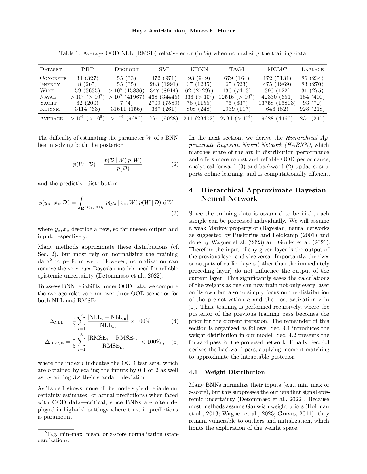
To assess BNN reliability under OOD data, we compute the average relative error over three OOD scenarios for both NLL and RMSE:

where the index i indicates the OOD test sets, which are obtained by scaling the inputs by 0.1 or 2 as well as by adding 3× their standard deviation.

As Table 1 shows, none of the models yield reliable uncertainty estimates (or actual predictions) when faced with OOD data-critical, since BNNs are often deployed in high-risk settings where trust in predictions is paramount.

In the next section, we derive the Hierarchical Approximate Bayesian Neural Network (HABNN), which matches state-of-the-art in-distribution performance and offers more robust and reliable OOD performance, analytical forward (3) and backward (2) updates, supports online learning, and is computationally efficient.

Since the training data is assumed to be i.i.d., each sample can be processed individually. We will assume a weak Markov property of (Bayesian) neural networks as suggested by Puskorius and Feldkamp (2001) and done by Wagner et al. (2023) and Goulet et al. (2021). Therefore the input of any given layer is the output of the previous layer and vice versa. Importantly, the sizes or outputs of earlier layers (other than the immediately preceding layer) do not influence the output of the current layer. This significantly eases the calculations of the weights as one can now train not only every layer on its own but also to simply focus on the distribution of the pre-activation a and the post-activation z in (1). Thus, training is performed recursively, where the posterior of the previous training pass becomes the prior for the current iteration. The remainder of this section is organized as follows: Sec. 4.1 introduces the weight distribution in our model. Sec. 4.2 presents the forward pass for the proposed network. Finally, Sec. 4.3 derives the backward pass, applying moment matching to approximate the intractable posterior.

Many BNNs normalize their inputs (e.g., min-max or z-score), but this suppresses the outliers that signal epistemic uncertainty (Detommaso et al., 2022). Because most methods assume Gaussian weight priors (Hoffman et al., 2013;Wagner et al., 2023;Graves, 2011), they remain vulnerable to outliers and initialization, which limits the exploration of the weight space.

Instead, we use a hierarchical Gaussian-Inverse-Gamma prior that marginalizes to a heavy-tailed Student’s t distribution (Taboga, 2017), and extend this to layerwise vectors via a Gaussian-Inverse-Wishart hyperprior for multivariate t’s. Since the t distribution does not belong to the exponential family, we apply assumed-density filtering-approximating both layer outputs and weight posteriors as (multivariate) Student’s t-and adopt a mean-field simplification, following Goulet et al. ( 2021)’s finding that posterior covariances effectively diagonalize. For a more detailed discussion of the weight distribution, see Appendix A.

Note that due to treating the layers sequentially, we will omit all layer indices to increase readability. In theory a rank-reducing linear transformation of a multivariate Student’s t-distribution would result in a Student’s t-distribution again (Taboga, 2017), however after the first layer the multiplicative non-linearity in Equation (1) distorts this. In order to overcome this issue, it will be assumed that p(a|D), i.e., the distribution of the preactivation a, will always be Student’s t-distributed for any given layer. In the following, a moment matching approach will be employed to estimate the parameters of the distribution. Luckily, both the mean and scale matrix have been derived by Wagner et al. (2023) for the Gaussian case already. These derivations also hold for Student’s t-distributions and therefore we will simply state the final formulae.

The elements of the mean vector are given by

where µ z is the mean of the post activation z of the previous layer, defined in Equation (1). Due to the mean-field assumption, both the scale and covariance matrix are diagonal.

The elements of the diagonal of the covariance matrix are then given by

with Tr(•) denoting the trace of a matrix, and C W and C z representing the covariance matrices of the weights W and the post-activation values z, respectively.

For a multivariate Student’s t-distribution the covariance matrix is not equal to the scale matrix but instead only defined if the degrees of freedom are greater than two.

In that case the covariance matrix can be calculated according to

with Σ being the scale matrix, ν the degrees of freedom, and C the covariance matrix. This implies that, in our case, the diagonal elements τ 2 a of the scale matrix of a can be computed as

In the first layer, the degrees of freedom remain unaffected by the linear transformation, so it was decided not to alter them in subsequent layers either.

This concludes the pre-activation calculations. The next step is the element-wise application of the ReLU function to the pre-activation a as defined in (1). Assuming a diagonal covariance structure, the mean and variance of each post-activation z = f (a) can be computed independently and later vectorized. Both the mean and scale are calculated analytically without any approximations. The detailed derivations can be found in Appendix B; here, we only state the final results. For clarity, we demonstrate the results for a single neuron z i = f (a i ), i = 1, . . . , M l+1 , omitting the index for readability. We also assume the parameters of a are given by µ, τ 2 , ν.

The mean value and variance of f (a) are then given by

Var[ f(a)] =:

respectively, where Γ is the Gamma function, F denotes the cumulative distribution function of a Student’s tdistributed random variable, and B is the Beta function, defined in the appendix in (25).

This section shifts focus from predicting y given an input x to updating the weights W using training data D. Under the assumption that training samples are i.i.d. and making use of the Markov property of (Bayesian) neural networks, weight updates can be performed in sequence. Consequently, samples are processed one at a time, eliminating the need for batch processing typically seen in neural network training. In this context, the posterior from the previous sample is used as the prior for the next one.

Updating the weights of a layer is performed in two steps: first, a l gets updated using z l+1 and then, W ⊤ l , z ⊤ l ⊤ gets updated using a l . Since we derive the update equations for both steps similarly, we denote both involved variables of each step as X 1 and X 2 . We assume that they are jointly multivariate Student’s t-distributed and we calculate the posterior p(X 1 |D) by marginalizing over X 2 , yielding

Unlike the Gaussian case, where the posterior (11) can be computed analytically (Wagner et al., 2023), this is not possible here because the product of two multivariate Student’s t probability density functions (PDFs) does not yield another multivariate Student’s t PDF.

To address this issue, we approximate the true posterior in Equation ( 11) by using a surrogate multivariate Student’s t-distribution, matching its moments to those of the true posterior. Similar to the forward pass, the calculations can now be done analytically without any approximations. We will again only state the final update formulae for the mean, scale matrix as well as the degrees of freedom. Interested readers are referred to Appendix C for the detailed derivations. The update formulae for the mean, scale matrix, and degrees of freedom are given by

respectively, with

i=1 (.) i being the sum over all elements of the vector. For the first step (updating a l by z l+1 ), the cross-scale matrix Σ 12 is equal to Σ a l z l+1 and can be calculated according to

Algorithm 1 Single training pass for HABNN

Calculate (µ a ) l i and (σ 2 a ) l i by Eq. ( 6) and ( 7) ∀i 4:

Calculate (µ z ) l i and (σ 2 z ) l i by Eq. ( 9) and ( 10) ∀i 5: end for 6: for l = L to 1 do 7:

Update µ l a|D , Σ l a|D and ν a|D by Eq. ( 12)-( 15)

8:

Update µ l W |D , Σ l W |D and ν W |D by Eq. ( 12)-( 14), ( 16)

Update µ l z|D , Σ l z|D and ν z|D by Eq. ( 12)-( 14), ( 16) 10: end for In the second step, when updating W ⊤ l , z ⊤ l ⊤ using a l , the cross-covariance matrix (not cross-scale matrix)

⊤ a l has already been derived by Wagner et al. (2023). It is given by

The scale matrix can then be obtained by rescaling the covariance matrix according to Equation ( 8).

In Alg. 1 HABNN is summarized. First, the parameters of the predictive distribution p(y|x) according to (3) are calculated in lines 2-5. The output value y is used to update the weights and thus, to calculate the weight posterior p(W |x, y) according to (11). This is performed in lines 6-10. Applying HABNN sequentially over all input-output pairs (x i , y i ) ∈ D, i = 1, . . . , N in a single run completes the training of the BNN.

Both KBNN and TAGI share the update formulas

for the mean and covariance matrix, respectively. Here, the mean update step ( 17) is identical to the mean update (12) of HABNN.

The covariance matrix update ( 18) is also similar to the scale matrix update (13) in HABNN, with one key difference: a scaling factor

precedes Σ 1|2 in HABNN. However, as the degrees of freedom ν approach infinity with an increasing number of training samples, this scaling factor converges to 1.

Consequently, in the limit of large degrees of freedom, the scale matrix update in HABNN becomes equivalent to the covariance update in TAGI and KBNN. As the Student’s t-distribution converges to a Gaussian one, the scale matrix of HABNN transitions to a covariance matrix, aligning both update steps fully.

Thus, HABNN generalizes both TAGI and KBNN, preserving their methodologies while extending their applicability through a more flexible prior structure.

Since HABNN employs a mean-field variational approximation over its weight vector of size n (i.e. the total number of individual network weights), it needs only to learn 2n+1 parameters in total: the mean and variance (or scale) for each of the n weights, plus a single global degrees-of-freedom parameter. Consequently, both its memory footprint and computational cost scale linearly in n. As shown in Table 4 (Appendix), this lean parameterization also makes HABNN the fastest model among those evaluated.

In this section, we will evaluate HABNN by comparing its performance to other state-of-the-art methods on UCI regression datasets as this is the standard benchmark for BNN models. This can be seen in the papers of for example Wagner et al.; Goulet et al.; Hernández-Lobato and Adams and many more. Additionally, we will analyze how effectively HABNN can handle out-ofdistribution data and how trustworthy its predictions are.

For all experiments, we will use a neural network with one hidden layer of size 50 and ReLU activation. The only exception is Laplace which was implemented with Tanh as its ReLU implementation diverged most of the time on most datasets (approx. 90% of the time).

The initial scale matrix for HABNN will be set as the identity matrix times 0.01, while the means will be initialized by drawing from a standard Gaussian distribution, following a similar approach to that used in Wagner et al. (2023). The initial degrees of freedom for the weights W will be set to 12.

All experiments have been conducted on a Intel Core i9-13950HX on a Lenovo P16 Gen2 laptop.

Six UCI datasets will be used to compare the performance of the different models: Concrete, Energy, Wine, Naval, Yacht, and Kin8nm. The datasets will be randomly split into training and test sets, with 90% of the data allocated for training and 10% for testing. Importantly, we will not perform any data preprocessing, as this can lead to overfitting, as previously discussed in Section 3 and further shown in the appendix. We will later demonstrate that avoiding data preprocessing can significantly enhance the models’ out-of-distribution performance. This is particularly important in highsecurity environments, where BNNs were designed to ensure reliable performance even when the underlying data-generating distribution may shift. For SVI, MCMC the implementation in Pyro (Bingham et al., 2019) is used, for PBP we use the Theano implementation of the original paper and Daxberger et al. ( 2021) for Laplace.

We train KBNN, TAGI, HABNN, PBP, and Dropout for one epoch each whereas SVI is trained for 250 epochs since it is used to batch over the whole training set.

For MCMC, we employ the No-U-Turn sampler and run sampling until 100 posterior draws are obtained, while for the Laplace approximation we perform one epoch of optimization to fit the point estimates of the weights and a second epoch to compute their variances.

In order to account for stochastic effects, we average the performance of the models on 100 runs and state their median RMSE and negative log-likelihood (NLL) as well as their OOD performance measured by ( 4) and (5), respectively. Remember that the OOD scenarios have been simulated by multiplying the test set by a factor of 0.1 and 2, or by adding three times the standard deviation of the test set. Note that the standard deviations are reported in Appendix H.

Tables 2 and3 No other method matches this level of across-the-board performance: PBP and SVI excel on some datasets but falter on others, TAGI and KBNN depend heavily on data normalization and degrade under extreme scales, MCMC and Laplace exhibit instability or variance collapse, and Dropout manages at most a single top-three finish across both metrics. HABNN’s heavy-tailed multivariate Student’s t prior fosters extensive exploration of the parameter space while its local Gaussian-like updates ensure precise convergence to high-probability posterior modes, thereby combining strong uncertainty quantification with competitive predictive accuracy in a way no other model achieves. This is further confirmed by the work of Fortuin et al. ( 2022), as they showed that BNNs with fully connected layers exhibit heavy-tailed weight distributions.

To assess HABNN’s practical utility, we evaluate it on the Industrial Benchmark (IB), a continuous-state, continuous-action, partially-observable environment explicitly designed to capture core challenges of real industrial control: delayed responses, rate-of-change limits on actuators, heteroscedastic sensor noise, latent drift, and multi-criteria reward trade-offs (Hein et al., 2017a).

Unlike classic reinforcement learning (RL) testbeds (e.g. CartPole, MountainCar), IB embeds realistic actuator constraints and noisy sensor observations that scale with latent state, forcing policies to remain adaptive over long horizons rather than converge to a fixed operating point (Hein et al., 2017a). A more detailed explanation about the benchmark as well as the experimental setup can be found in Appendix I.

Recent work introduced a Model Predictive Control + Active Learning framework that uses online uncertainty estimates to sample next states where the model is most uncertain, achieving large gains in sample efficiency on IB (Wu et al., 2024). Adopting a similar uncertaintyaware strategy, we compare HABNN to standard RL baselines-A2C, TD3, and SAC-from Stable Baselines (Hill et al., 2018).

Figure 1 shows that HABNN achieves the lowest and most stable one-step prediction loss on IB compared to standard baselines (A2C, TD3, SAC). From the first timesteps, HABNN drives its mean-squared error into the 300-400 range and holds it there throughout training, whereas the baselines start above 380 and either plateau at higher loss levels or exhibit sharp spikes under IB’s noisy, non-stationary dynamics. Both TD3 and SAC struggle with heteroscedastic sensor noise and actuator delays-spiking in loss as they attempt to average out disturbances-while A2C converges more slowly and never matches HABNN’s lowloss regime.

These results confirm that HABNN’s uncertainty-aware sampling, powered by heavy-tailed Student’s t priors and a latent-drift model, yields far more sample-efficient and robust system identification, achieving and sustaining low prediction error with orders of magnitude fewer interactions.

HABNN’s tractability relies on two main approximations. In the forward pass, we fit a Student’s t distribution-ignoring alternative families and higher moments-a strategy common to most non-sampling BNNs. In the backward pass, we assume that preactivations (a l ), post-activations (z l ), weights, and previous-layer inputs (z l-1 ) are jointly multivariate Student’s t, which admits closed-form updates but may misrepresent complex posteriors. Performance can degrade if a high-probability mode lies near the initialization; in practice, increasing the degrees of freedom ν restores Gaussian behavior. For very deep networks, the heavy tails at initialization may still induce instability, suggesting that layer-wise ν schedules or adaptive update rates could be useful.

We presented the Hierarchical Approximate Bayesian Neural Network (HABNN), which offers analytical forward and backward passes with linear complexity in the number of weights.

HABNN

Most BNNs model the weights as Gaussian distributed (Hoffman et al., 2013;Wagner et al., 2023;Graves, 2011). This is, however, worrying as a Gaussian distribution puts a lot of probability mass around its mean due to its exponential decay. This in turn makes it challenging for the model to effectively explore its parameter space in depth. As a result, the models become highly sensitive to their initializations and struggle to fit the data effectively if the posterior mode is far from the initialization.

To effectively address this issue, we will introduce a hierarchical distribution for the weights. We will add a Gaussian-inverse-gamma distribution on top of the Gaussian distribution of the weights. This means that the weights will be distributed according to

where the latter Gaussian-inverse-gamma distribution is defined as follows:

• µ W represents the mean of the weight distribution and, given the variance σ 2 W , follows

• σ 2 W follows an inverse-gamma distribution with shape parameter α and scale parameter β according to

This distribution is a common prior for variance in Bayesian inference, particularly when the variance is uncertain.

It can now easily be shown that the resulting distribution of the weights will be a Student’s t-distribution (Taboga, 2017). The Student’s t-distribution is characterized by heavier tails than the normal distribution, making it more robust to outliers. It is commonly used to model data with greater variability or when dealing with small sample sizes. As the degrees of freedom ν increases, the Student’s t-distribution approaches a normal distribution. This is one of the fundamental properties of the Student’s t-distribution, allowing it to be particularly useful in Bayesian statistics as it can model the data with robustness to extreme values in the early stages of training.

As layers of (Bayesian) neural networks typically consist of more than one weight due to multiple inputs to a layer, we will assume a joint Gaussian distribution with a Gaussian-inverse-Wishart hyperprior distribution.

This, in turn, will result in multivariate Student’s t-distributions for the weights, which is defined by the probability density function (PDF)

where µ is the location, Σ the scale matrix, and ν represents the degrees of freedom.

As the Student’s t-distribution does not belong to the Exponential family, there exists no conjugate prior for this distribution. Thus, there is no analytical solution to Equations ( 2) and ( 3). Instead we follow an assumed density approach where we assume a (multivariate) Student’s t-distribution for the output z l of any given layer and for the posterior distribution of the weights W l of that layer.

As weights in a given layer of a BNN become independent over time, it is common to assume their independence from the outset. This approach, known as the mean-field assumption, simplifies computations by treating all weights as uncorrelated, effectively setting non-diagonal elements of the covariance matrices to zero. Adopting this assumption not only increases scalability but also aligns with observations made by Goulet et al. ( 2021), who demonstrated that the covariance matrix of the posterior tends to converge toward a diagonal form.

The PDF of the Student’s t-distribution with ν degrees of freedom, location parameter µ, and scale parameter σ 2 is given by

where Γ(•) is the gamma function. The multivariate t-distribution is defined by the PDF

where µ is the location, Σ the scale matrix, and ν represents the degrees of freedom. Note that for the remainder of the text we will also refer to the location (parameter) as mean.

Given that a follows a Student’s t-distribution, we assume the parameters are defined by µ, τ 2 , and ν, representing the mean, scale, and degrees of freedom, respectively. We will omit the quantity D to ease the notation. The mean µ z of the post-activation is then given by

with F (0 | µ, τ 2 , ν) being the cumulative distribution function of the random variable a. This can easily be seen by simply resubstituting a = x + µ into the integral.

The first integral in ( 19) can now be approached similarly to calculating the expected value of a Student’s t-distributed random variable. By substituting u = 1 + x 2 ντ 2 one obtains

Combining Equation ( 19) and Equation ( 20) results in the final formula

This sums up the calculation of the mean and we will turn our attention towards the scale matrix in the following.

The most convenient way to calculate the scale parameter is by actually calculating the variance and then rescaling it according to Equation ( 8). Therefore, we need to compute the variance σ 2 z of f (a) next. With the mean already derived, it is sufficient to merely calculate the (non-central) second-order moment E[ f(a) 2 ], which is equal to σ 2 z + µ 2 z . Reformulating the latter then gives the desired variance σ 2 z . To simplify the notation, we will temporarily omit the scaling factor of the density and include it later. Hence, one obtains

which can now be evaluated by substituting x = a -µ again, resulting in

After expanding the binomial term one obtains

where the integrals in II and III have already been calculated in Equation ( 20) and Equation ( 19), respectively.

Thus, the only one remaining is I. It can be handled by partitioning the domain of integration according to

The first integral can now be solved similarly to calculating the variance of a Student’s t-distributed random variable. By splitting the two terms in the integral, one obtains

with B(•) being the Beta function. Note that we use the first definition of the Beta function, which is defined as

Exploiting the close relationship between the Beta function and the Gamma function yields

where we used the fact that

. Now, all that is left is to calculate the second summand in Equation ( 23). As both cases can be calculated similarly, w.l.o.g we will assume µ ≥ 0. One can split up the two terms in the integral just like before and use the same substitution as in Equation ( 24) to get

The last term can now be recognized as the definition of the incomplete beta function, denoted by B µ 2

Unlike the complete beta function, the incomplete beta function evaluates the integral only up to the argument, rather than over the entire range. Hence, it is defined as

Combining all of the terms and simplifying them now results in

where i is defined as

Combining ( 21) with ( 26) yields the variance of f(a) according to

Recall that this is not the final scale parameter but rather the variance, which needs to be rescaled according to Equation ( 8) in order to obtain the actual scale parameter.

We assume that the degrees of freedom remain unaltered as the ReLU function is mostly linear and linear transformations do not change the degrees of freedom of a Student’s t-distributed random variable.

For the output layer l = L, the variance σ 2 ϵ of the Gaussian noise ϵ is added to the variance σ 2 z of ( 27) to account for the aleatoric uncertainty of the data.

Central to the approach presented here is the conditional distribution of a partitioned multivariate t-distribution.

Let X follow a multivariate t-distribution with the partition

where

and d i being the dimension of X i holds.

In the first scenario, we aim to update the pre-activation a l using z l+1 . The cross-scale matrix Σ a l z l+1 can be calculated according to

In the second case, when updating W ⊤ l , z ⊤ l ⊤ using a l , the cross-covariance matrix (not cross-scale matrix)

⊤ a l has already been derived by Wagner et al. (2023). It is given by

The scale matrix can then be obtained by rescaling the covariance matrix according to Equation (8). Attentive readers will notice that µ 1|2 and Σ 1|2 are the parameters of a conditional distribution of a multivariate Gaussian distribution. As the degrees of freedom increase (by d 2 for every sample), the scaling factor of the scale matrix will converge to one. As a multivariate Student’s t-distribution converges to a multivariate Gaussian distribution as the degrees of freedom increase (Roth, 2012), the conditional distribution of a multivariate Student’s t-distribution similarly approaches that of a multivariate Gaussian distribution.

Since KBNN and TAGI use a comparable training framework with Gaussian distributions, the update steps in HABNN will likewise converge to those of KBNN and TAGI. This can also be formally demonstrated once the final backward propagation formulas have been derived.

To calculate the posterior of X 1 , we marginalize over X 2 , yielding

Unlike the Gaussian case, where the posterior (31) can be computed analytically (Wagner et al., 2023), this is not possible here because the product of two multivariate t probability density functions (PDFs) does not yield another multivariate t PDF. To address this issue, we approximate the true posterior in Equation ( 31) by using a surrogate multivariate t-distribution, matching its moments to those of the true posterior. In both cases considered, we will assume a joint multivariate t-distribution for all of the random variables.

This means that we will assume that X 1 := a l and X 2 := z l+1 are jointly multivariate t-distributed in the first case and X 1 := W ⊤ l , z ⊤ l ⊤ and X 2 := a l are also jointly multivariate t-distributed in the second case. This implies that the moments of the posterior can be derived in a general form using the random variables X 1 and X 2 . Subsequently, the update formula can be adjusted based on the specific parameters being updated at any given point.

In both cases considered, we will assume a joint multivariate t-distribution for all of the random variables. This means that we will assume that X 1 := a l and X 2 := z l+1 are jointly multivariate t-distributed in the first case and X 1 := W ⊤ l , z ⊤ l ⊤ and X 2 := a l are also jointly multivariate t-distributed in the second case. This implies that the moments of the posterior can be derived in a general form using the random variables X 1 and X 2 . Subsequently, the update formula can be adjusted based on the specific parameters being updated at any given point.

We will start off by calculation the mean, which is given as

where a) has been obtained by marginalizing the posterior density over X 2 and b) by switching the orders of integration. This can be done as the conditions for Tonelli’s theorem (Halmos, 1950) for non-negative measurable functions are obviously met. Recall that the parameters of a conditional multivariate t-distribution are given by Equation ( 28). Similary, the update steps of the weights W are given by

And the ones of the post-activation z by

For l = L, this backward recursion commences from µ z l+1 = y and Σ z l+1 = 0 .

As we assess the performance of these models, it is crucial to consider training times. Given that different models utilize varying batch sizes, we will calculate each model’s training time by iterating through the dataset sample by sample, updating the model after each pass. However, this approach presents a challenge for PBP, as its implementation requires a minimum of two samples for training. Consequently, we chose to iterate through the entire dataset using a batch size of 2, without any additional adjustments to the training time.

It’s important to note that the training times for TAGI are excluded from this analysis because its current implementation is not compatible with Windows, necessitating the use of virtual machines. This limitation significantly impacts its performance, making a fair comparison impossible.

As shown in Table 4, KBNN and HABNN exhibit remarkable speed and significantly outperform all other models, thanks to their analytical expressions for both the forward and backward passes, which eliminate the need for costly gradient calculations. Although HABNN requires more complex computations for its forward pass, it remains faster than KBNN due to its efficient diagonal covariance structure. It is quite revealing to note how slow PBP can be. Interestingly, it operates efficiently when it processes the entire training set at once, likely due to its backend being implemented in C++, which significantly accelerates the training process. In this scenario, the training times (in seconds) for the datasets are as follows: Concrete (2.07), Energy (1.71), Wine (2.99),Naval (3.822),Yacht (1.61),and Kin8nm (2.99). However, once we account for this effect by iterating through the training set sample by sample, its performance drastically declines.

Unlike traditional neural networks, BNNs employ random variables as weights, typically doubling the number of learnable parameters. This raises the question of whether and how different weight initializations affect the model’s final performance. To explore this, we evaluated HABNN’s sensitivity to weight and degrees of freedom initializations by conducting experiments with varying initial scale parameters and degrees of freedom for the weights. In these experiments, we set the scale parameters to 0.01, 0.1, 1, 2, and 5 and the degrees of freedom to 12, 20, 30, 50, and 75, measuring their impact on model performance across different datasets.

Tables 5 and6 demonstrate that HABNN exhibits remarkable robustness across most datasets, with only slight variations in performance. This consistent stability further reinforces HABNN’s status as a highly robust model capable of adapting to diverse conditions. The primary exception is observed in the naval dataset when the initial scale parameter is significantly high. This behavior could be attributed to the model’s enhanced exploration due to its heavier tails combined with the elevated initial scale, making it challenging to converge effectively in the presence of the naval dataset’s high feature values. Further investigation is required to validate and explore this hypothesis in greater detail.

We also evaluated HABNN on architectures with 1 to 4 hidden layers, each containing 50 neurons. The experiments were conducted with different degrees of freedom and varying initializations of the scale parameter. As shown in Table 7, the single-hidden-layer architecture performs best in most cases, except for the Concrete and Yacht datasets, where the two-layer architecture closely matches or even exceeds its performance. Notably, only the four-layer model exhibits a decline in performance, likely due to overfitting on these relatively simple datasets.

While adjusting the number of hidden neurons per layer might have improved results for deeper architectures, this was beyond the scope of our study, which primarily focuses on demonstrating the stability of HABNN.

Below you can find the full experiments that were used to derive the results in the main body of the paper.

In this subsection we will look at the in-distribution performance of all of the BNNs considered. The training data has not been normalized and the testing data has not been rescaled or changed in any way. The architecture and training methods are the same as in the main body of the paper.

Here are the OOD experiments in which the data has not been normalized. This means that we have not normalized the training data and have then looked at the OOD performance of all the BNNs considered. Remember that we looked at 3 OOD settings, namely rescaling the test set by a factor of 0.1 and 2 or by adding three times the standard deviation of the test set onto itself. The results can be found in the Tables 10, 11 and12.

In this section we will report the full experiments when the data has been normalized. Again, the network architecture as well as the hyperparameters stayed the same as reported in the main body of the paper. The results can be found in the Tables 13141516.

Below you can find the respective standard deviations of the BNNs, for the experiments in which the training data has not been normalized. We will report the standard deviations of the actual RMSE (NLL) values, as well as the average relative RMSE (NLL) errors. The results are reported in the Tables 17181920.

In our Industrial Benchmark (IB) experiments, we define the per-timestep loss as

where c t denotes consumption and f t fatigue. With the environment set to the worst-case setpoint of 100, an effective loss typically falls in the range 230-400.

For comparison, the original IB authors report achieving a loss of approximately 230 after training for over 100,000 timesteps on 96 CPUs-using histories of 10-30 past observations and roughly one week of runtime Hein et al. (2017b). By contrast, our HABNN model uses only the current sample (no history), a single hidden layer of 80 units, degrees of freedom initialized at 12, and a weight-scale of 0.01. Despite this much lighter training regime, we are able to approach competitive performance. The results presented have been averaged over 100 runs.

%-second only to PBP’s 7.26 %. For NLL, HABNN similarly attains 3rd on Concrete (13 %), 2nd on Energy (40 %), 2nd on Wine (29 %), 2nd on Naval (65 %), 3rd on Yacht (27 %), and 1st on Kin8nm (22 %), resulting in an average NLL error of 3.72 %, again ranking second overall.

E.g. min-max, mean, or z-score normalization (standardization).