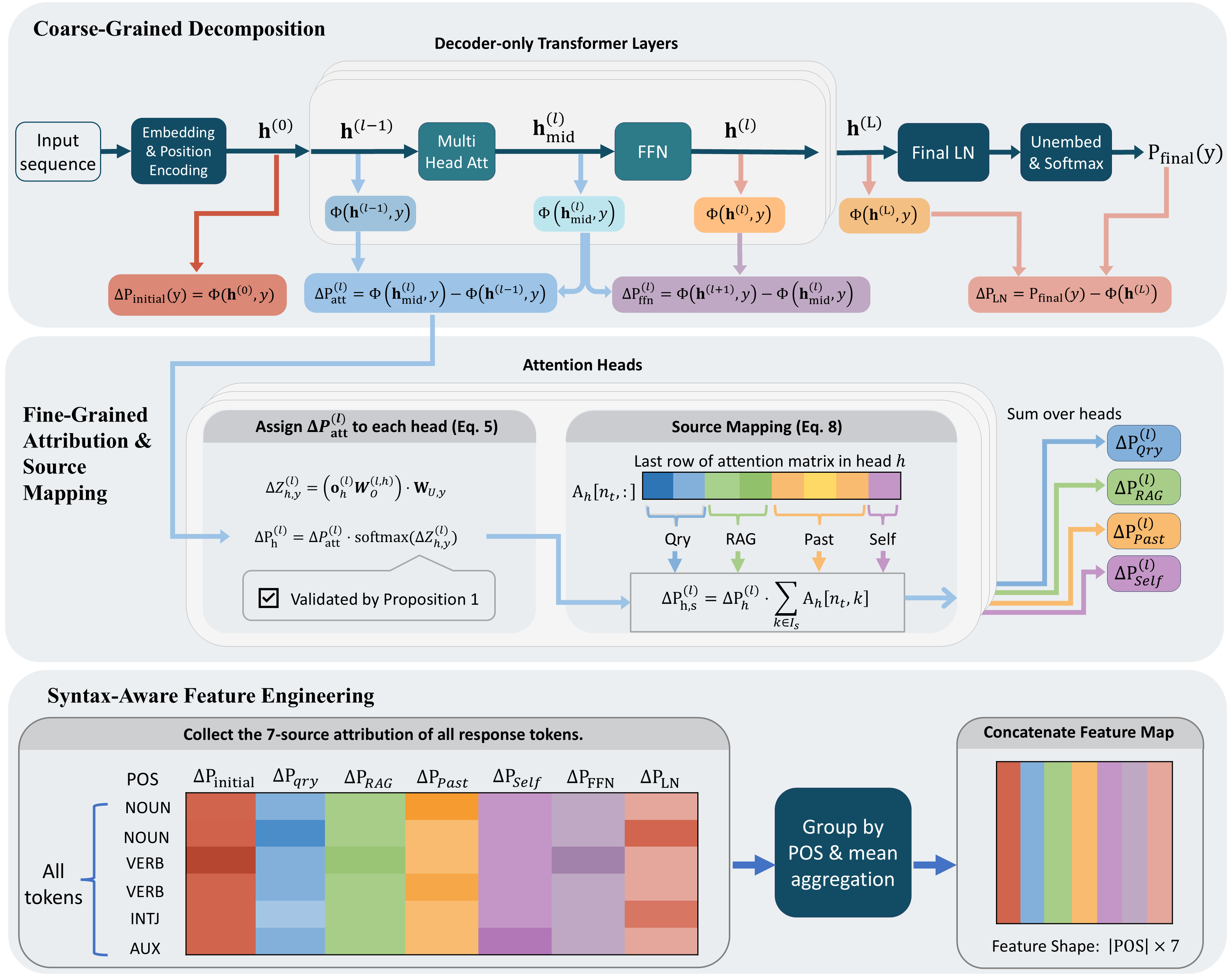
Detecting hallucinations in Retrieval-Augmented Generation remains a challenge. Prior approaches attribute hallucinations to a binary conflict between internal knowledge stored in FFNs and the retrieved context. However, this perspective is incomplete, failing to account for the impact of other components of the LLM, such as the user query, previously generated tokens, the self token, and the final LayerNorm adjustment. To comprehensively capture the impact of these components on hallucination detection, we propose TPA which mathematically attributes each token's probability to seven distinct sources: Query, RAG Context, Past Token, Self Token, FFN, Final LayerNorm, and Initial Embedding. This attribution quantifies how each source contributes to the generation of the next token. Specifically, we aggregate these attribution scores by Part-of-Speech (POS) tags to quantify the contribution of each model component to the generation of specific linguistic categories within a response. By leveraging these patterns, such as detecting anomalies where Nouns rely heavily on LayerNorm, TPA effectively identifies hallucinated responses. Extensive experiments show that TPA achieves state-of-the-art performance.
Large Language Models (LLMs), despite their impressive capabilities, are prone to hallucinations (Huang et al., 2025). Consequently, Retrieval-Augmented Generation (RAG) (Lewis et al., 2020) is widely used to alleviate hallucinations by grounding models in external knowledge. However, RAG systems are not perfect. They can still hallucinate by ignoring or misinterpreting the retrieved information (Sun et al., 2025). Detecting such failures is therefore a critical challenge. * Corresponding author.
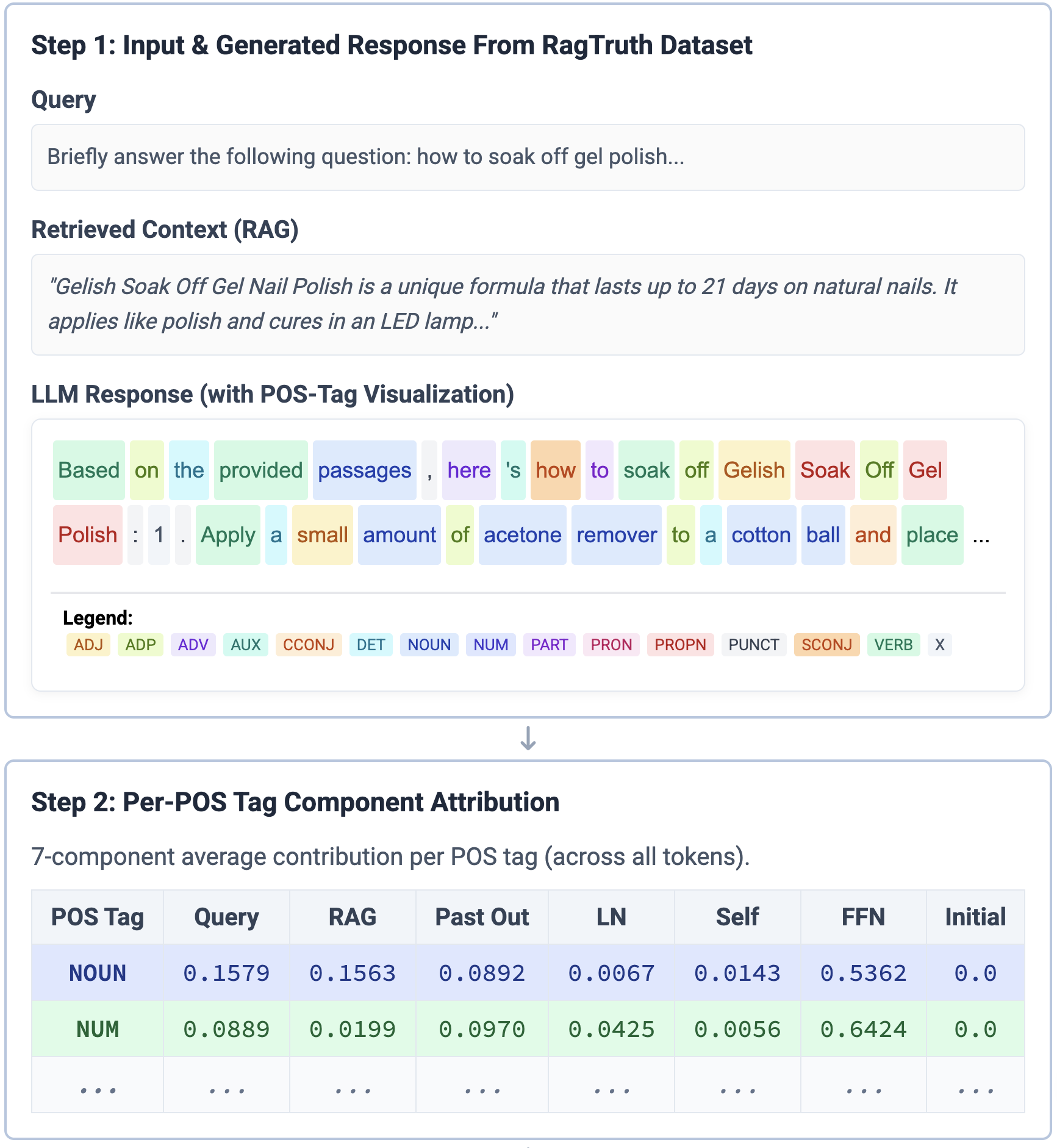
(a) TPA attributes each next-token probability to seven sources, then aggregates source attributions by POS tags to form the features for detecting hallucination.
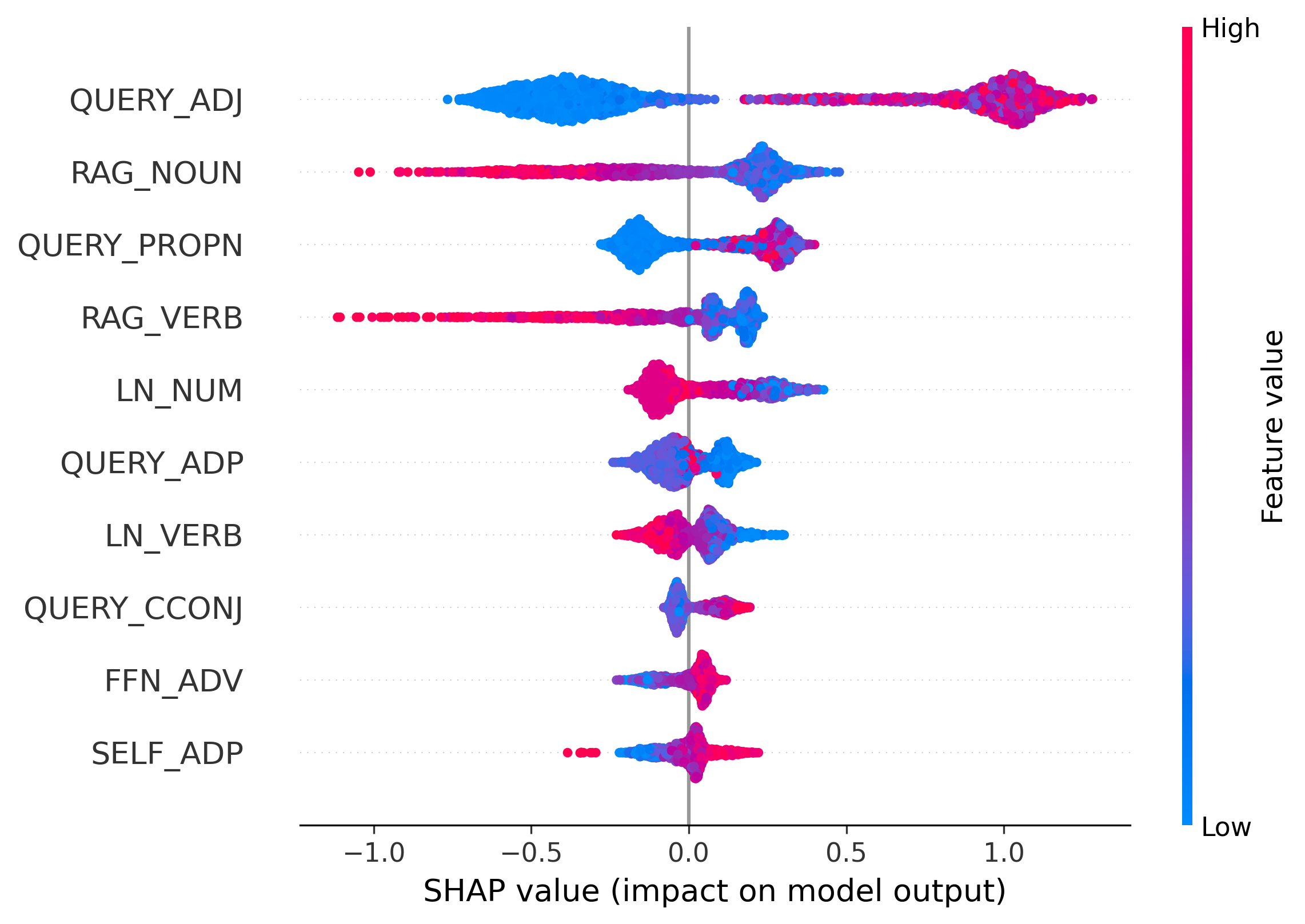
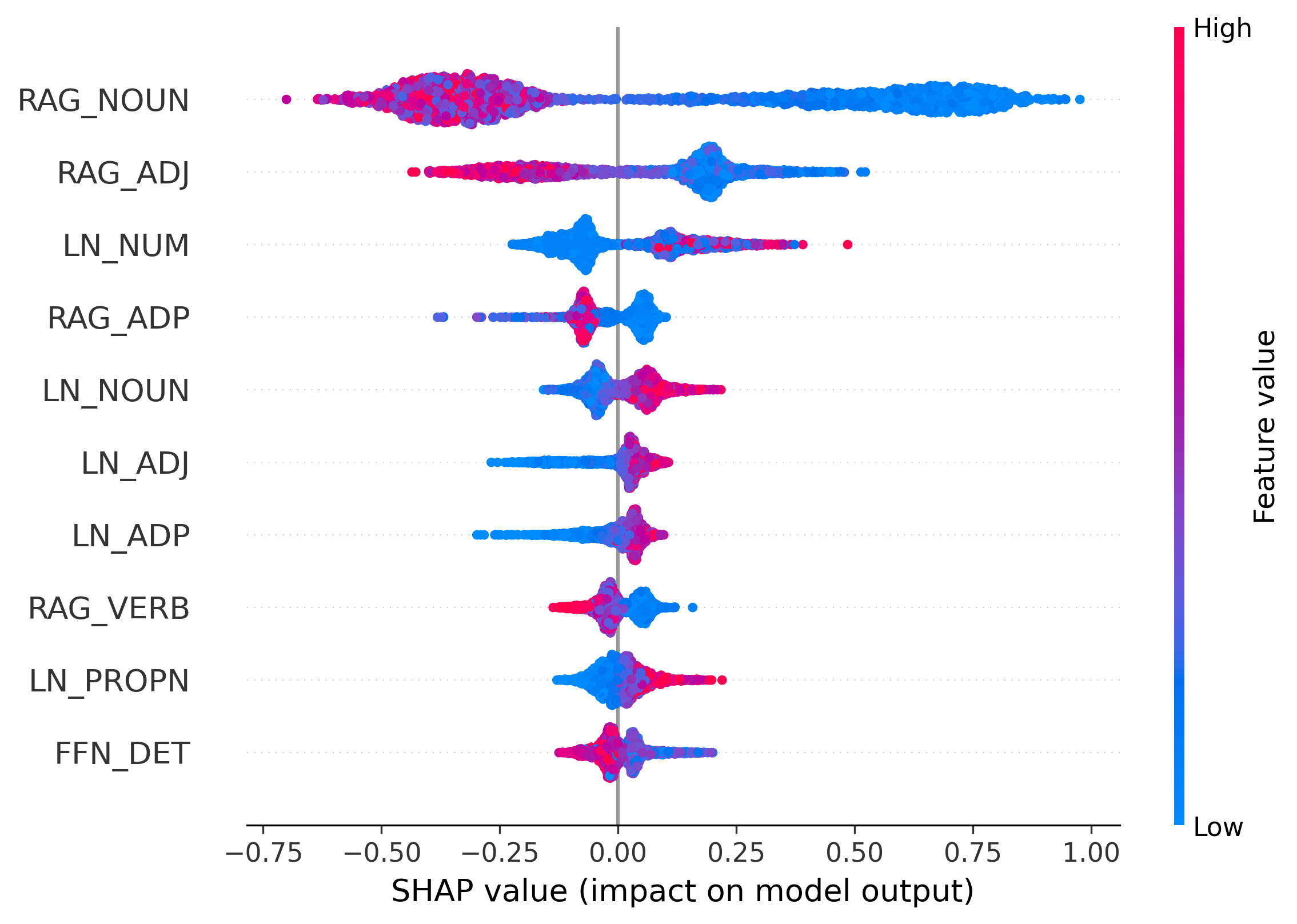
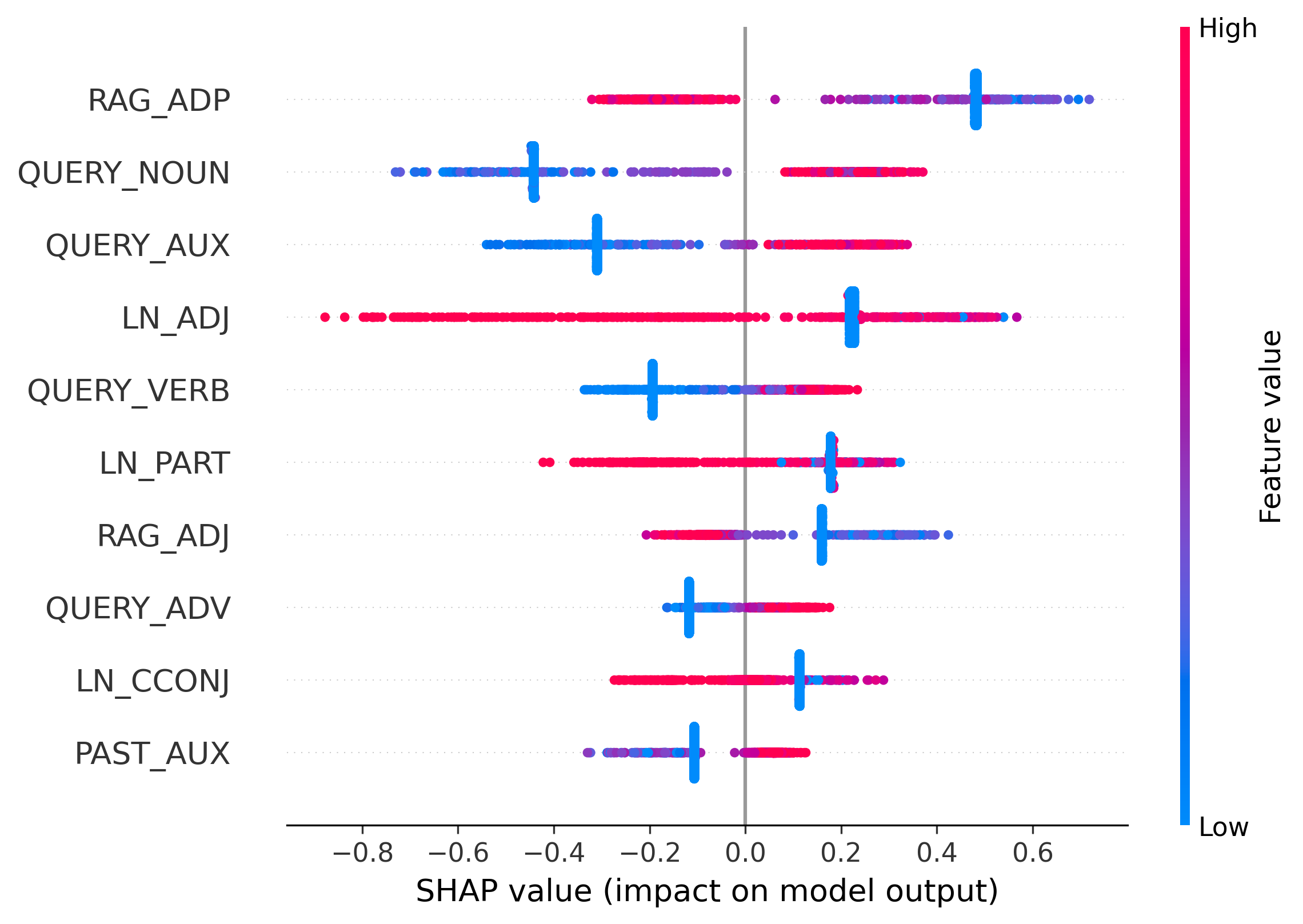
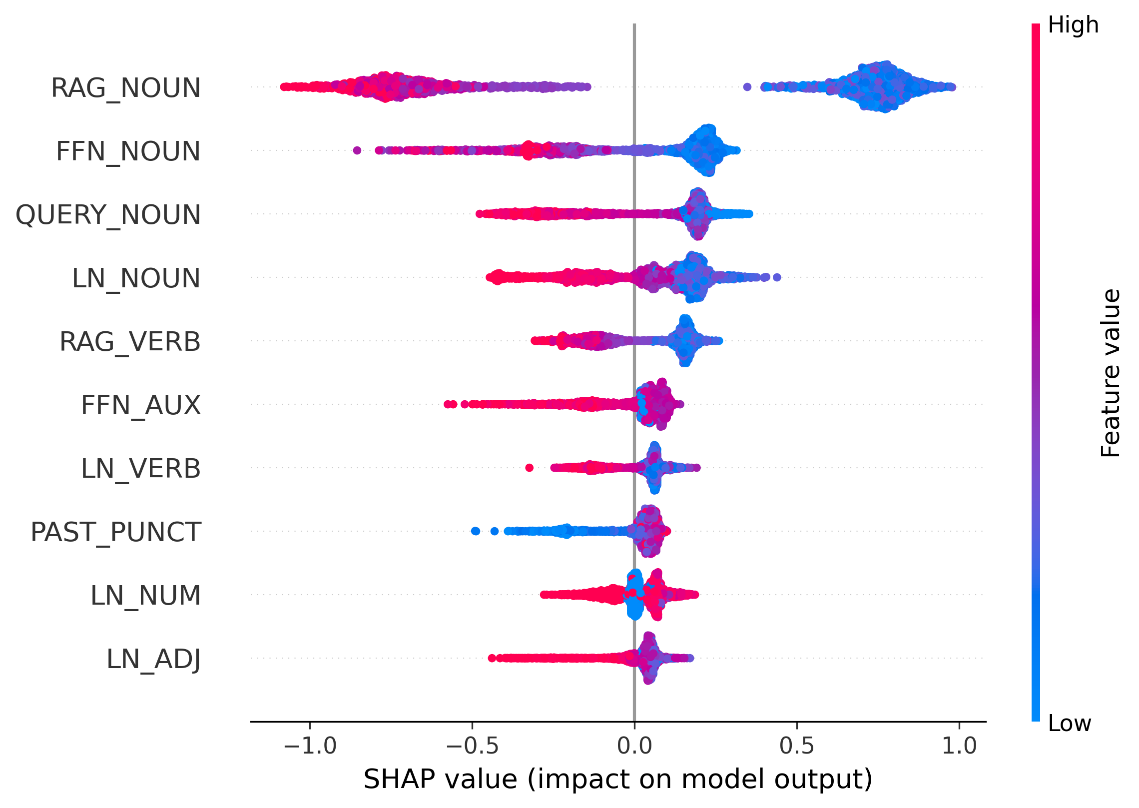
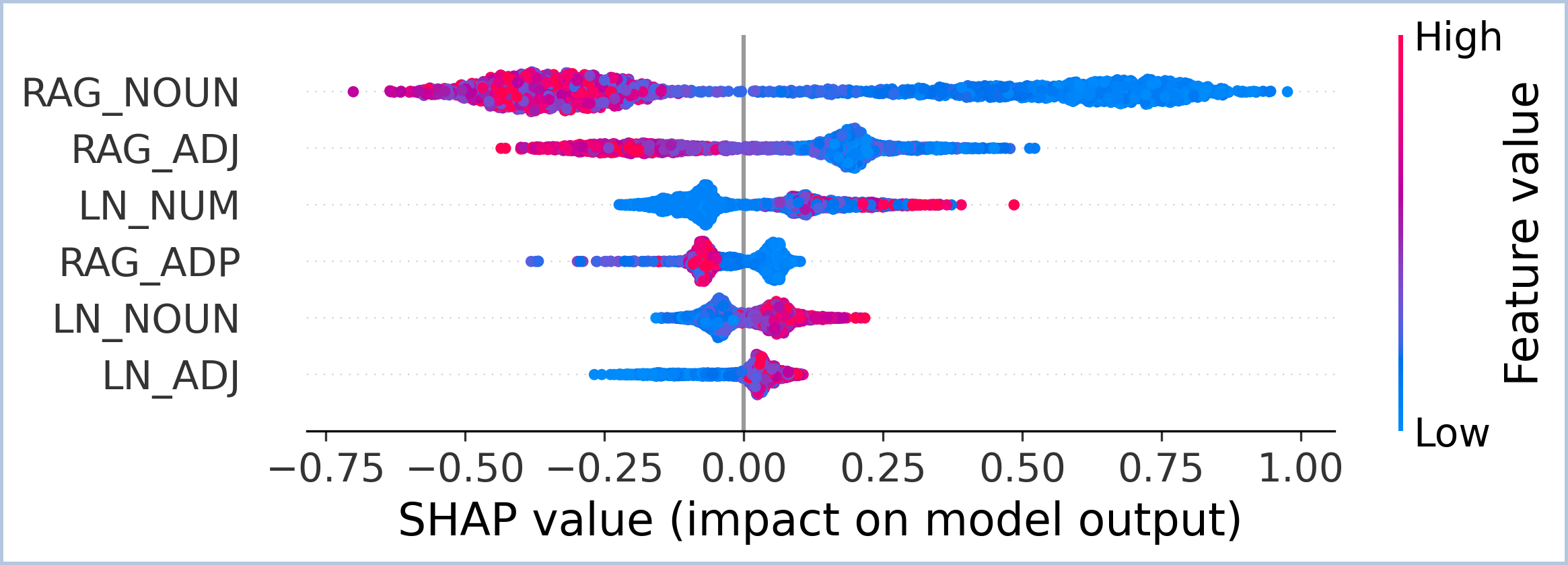
(b) Feature-importance analysis (SHAP) shows that the detector leverages source contributions conditioned on POS tags. For example, responses are more likely to be hallucinated when RAG contributes little to NOUN tokens or when LN contributes too much to NUM tokens.
Figure 1: Applying the TPA framework to a Llama2-7b response from RAGTruth dataset (Niu et al., 2024).
The prevailing paradigm for hallucination detection typically relies on hand-crafted proxy signals. For example, common approaches detect hallucination through consistency checks (Manakul et al., 2023) or scalar uncertainty metrics such as semantic entropy (Han et al., 2024). However, these methods only measure the symptoms of hallucination, such as output variance or surface confidence, rather than the underlying architectural causes. Consequently, they often fail when a model is confidently incorrect (Simhi et al., 2025).
To address the root cause of hallucination, recent research has shifted focus to the model’s internal representations. Pioneering works such as ReDeEP (Sun et al., 2025) explicitly assume the RAG context is correct. They reveal that hallucinations in RAG typically stem from a disproportionate dominance of internal parametric knowledge (stored in FFNs) over the retrieved external context.
This insight inspires a fundamental question: Is the binary conflict between FFNs and RAG the only cause of hallucination? Critical components like LayerNorm and User Query are often overlooked. Do contributions from these sources also drive hallucinations? In this paper, we extend the analysis to cover all additive components along the transformer residual stream. This approach enables detection based on the model’s full internal mechanics instead of relying on partial proxy signals.
To achieve this, we also assume the RAG context contains relevant information and introduce TPA (Next Token Probability Attribution for Detecting Hallucinations in RAG). This framework mathematically attributes the final probability of each token to seven distinct sources: Query, RAG, Past, Self Token, FFN, Final LayerNorm, and Initial Embedding. The attribution scores of these seven parts sum to the token’s final probability, ensuring we capture the complete generation process.
To compute these attributions, we proposed a probe function similar with nostalgebraist (2020) that uses the model’s unembedding matrix to read out the next-token probability directly from an intermediate residual-stream state. Concretely, for each component on the residual stream, we define its contribution as the change in the probed next-token probability before versus after applying that component. In this way, we can compute the contribution from Initial Embedding, attention block, FFN, and Final LayerNorm. For the attention block, we further distribute its contribution to Query, RAG, Past and Self Token according to their attention weights.
However, these attention scores are insufficient for detection. A high reliance on internal parametric knowledge (FFNs) does not necessarily imply a hallucination. This pattern is expected for function words like “the” or “of”. Yet, it becomes highly sus-picious when found in named entities. Therefore, treating all tokens equally fails to capture these critical distinctions.
To capture this distinction, we aggregate the attribution scores using Part-of-Speech (POS) tags. We employ POS tags to capture comprehensive syntactic patterns. Unlike Named Entity Recognition (NER), which is limited to specific entity types, POS tagging covers all tokens (including critical categories like Numerals and Adpositions) and maintains high computational efficiency.
Figure 1 illustrates how TPA turns a single response into detection features: we first compute token-level source attributions, then aggregate them by POS tags. The second step is critical since hallucination signals vary across distinct parts of speech. For example, low RAG contribution on nouns or high LN contribution on numerals is often indicative of hallucination. These patterns are harder to capture if we only use raw token-level attribution scores without POS information.
Our main contributions are:
-
We propose TPA, a novel framework that mathematically attributes each token’s probability to seven distinct attribution sources. This provides a comprehensive mechanistic view of the token generation process.
-
We introduce a syntax-aware aggregation mechanism. By quantifying how attribution sources drive distinct parts of speech, this approach enables the detector to pinpoint anomalies in specific entities while ignoring benign grammatical patterns.
Extensive experiments demonstrate that TPA achieves state-of-the-art performance. Our framework also offers transparent interpretability, automatically uncovering novel mechanistic signatures, such as anomalous LayerNorm contributions, that extend beyond the traditional FFN-RAG binary conflict.
Uncertainty and Proxy Metrics. Approaches in this category estimate hallucination via output inconsistency or proxy signals. Some methods quantify uncertainty using model ensembles (Malinin and Gales, 2021) or by measuring self-consistency across multiple sampled generations from a single model (Manakul et al., 2023). Others utilize lightweight proxy scores computable from a single generation pass, such as energy-based OOD proxy scores (Liu et al., 2020), embedding-based distance scores for conditional LMs (Ren et al., 2023), and token-level uncertainty heuristics for hallucination detection (Lee et al., 2024;Zhang et al., 2023). While efficient, these scores provide indirect signals (e.g., confidence or distribution shift) and therefore may be imperfect indicators of factual correctness.
LLM-based Evaluation. External LLMs are also employed as verifiers. In RAG settings, outputs can be checked against retrieved evidence (Friel and Sanyal, 2023) or through claim extraction and reference-based verification (Hu et al., 2024), and LLM-as-a-judge baselines are often instantiated using curated prompts (Niu et al., 2024). Automated evaluation suites (Es et al., 2024;True-Lens, 2024) have also been developed. Other strategies include cross-examination to expose inconsistencies (Cohen et al., 2023;Yehuda et al., 2024) or fine-tuning detectors for span-level localization (Su et al., 2025). However, many of these approaches require extra LLM calls or multi-step verification.
Probing Internal Activations. Recent work extracts factuality signals from internal representations, e.g., linear truthful directions or inferencetime shifts (Burns et al., 2022;Li et al., 2023), and probe-based detectors trained on hidden states (Azaria and Mitchell, 2023;Han et al., 2024). Related studies show internal states remain predictive for hallucination detection (Chen et al., 2024). Beyond detection, mechanistic analyses conflicts between FFN and RAG context (Sun et al., 2025), and lightweight indicators use attention-head norms (Ho et al., 2025). Active approaches steer or edit activations (Park et al., 2025;Li et al., 2023), or adjust decoding probabilities for diagnosis (Chen et al., 2025). In contrast, we decompose the final token probability into fine-grained sources.
As illustrated in Figure 2, TPA operates in three stages and can be implemented with a fully parallel teacher-forced pass. Given the generated response sequence y of length T , we can feed the entire sequence into the model with standard causal masking to extract hidden states and attention maps for all T tokens in a single teacher-forced pass. This avoids autoregressive resampling while enabling efficient attribution computation. We first derive a complete decomposition of token probabilities (Sec. 3.2), then attribute attention contributions to specific attribution sources (Sec. 3.3). Finally, we aggregate these scores to quantify how sources drive distinct parts of speech (Sec. 3.4). The pseudo-code and complexity analysis are provided in the Appendix. We report complexity instead of wall-clock time since the latter varies in different implementation hardware. To provide the theoretical basis for our method, we first formalize the transformer’s architecture.
We consider a standard decoder-only Transformer with L layers. We denote the query tokens as x qry , the retrieved context tokens as x rag , and the generated response as y = (y 1 , . . . , y T ), with prompt length T 0 = |x qry | + |x rag |. We analyze generation at step t ∈ {1, . . . , T }, where the model observes the prefix s t = [x qry , x rag , y 1 , . . . , y t-1 ], and predicts the next token y t . Let n t = |s t | = T 0 + t -1 denote the position index of the last token in s t (the token whose embedding is used to predict y t ).
Unless stated otherwise, all hidden states and residual outputs (e.g., h (l) , h (l) mid ) refer to the vector at the last position n t , and we omit the explicit index n t and the step index t for clarity. We keep explicit indices only for attention weights (e.g., A (l) h [n t , k]). We use d for the hidden dimension, H for the number of attention heads, and d h = d/H for the head dimension.
The input tokens are mapped to continuous vectors via an embedding matrix W e ∈ R |V|×d and summed with positional embeddings. The initial state at the target position is h (0) = W e [s t [n t ]] + p nt , where p nt is the positional embedding at position n t . We adopt the Pre-LN configuration. Crucially, each layer l updates the hidden state via additive residual connections:
(1)
Here, Attn(•) denotes the attention output vector at position n t under causal masking. This structure implies that the final representation is the sum of the initial embedding and all subsequent layer updates. To quantify these updates, we define a Probe Function Φ(h, y) similar to the logit lens technique (nostalgebraist, 2020) that measures the hypothetical probability of the target token y given any intermediate state vector h:
where W U is the unembedding matrix.
Guiding Question: Since the model is a stack of residual updates, can we mathematically decompose the final probability exactly into the sum of component contributions?
We answer the preceding question affirmatively by leveraging the additive nature of the residual updates. Based on the probe function Φ(h, y) defined in Eq. (3), we isolate the probability contribution of each model component as the distinct change it induces in the probe output.
We define the baseline contribution from input static embeddings (∆P initial ), the incremental gains from Attention and FFN blocks in layer l (∆P
ffn ), and the adjustment from the final LayerNorm (∆P LN ) as follows:
)
We define P final (y) as the model output probability after applying the final LayerNorm at position n t . By summing these differences, we derive the complete decomposition of the model’s output. Theorem 1 (Complete Probability Decomposition). The final probability for a target token y is exactly the sum of the contribution from the initial embedding, the cumulative contributions from Attention and FFN blocks across all L layers, and the adjustment from the final LayerNorm:
Proof. See Appendix.
The Guiding Question: While Eq. ( 8) quantifies how much the model components contribute to the prediction probability, it treats the term ∆P (l) att as a black box. To effectively detect hallucinations, we must identify where this attention is focused.
To identify the focus of attention, we must decompose the attention contribution ∆P (l) att into contributions from individual attention heads.
Standard Multi-Head Attention concatenates the outputs of H independent heads and projects them via an output matrix W O into head-specific sub-matrices, this operation is strictly equivalent to the sum of projected head outputs:
where o (l) h is the head output vector at the target position, derived from the attention row A (l) h [n t , :] and the value matrix V (l) h . Eq. ( 9) establishes that the attention output is linear with respect to individual heads in the hidden state space. However, our goal is to attribute the probability change ∆P (l) att to each head h. Since the probe function Φ(•) employs a non-linear Softmax operation, the sum of probability changes calculated by probing individual heads does not equal the attention block contribution. This inequality prevents us from calculating head contributions by simply probing each head individually, motivating our shift to the logit space.
To bypass the non-linearity of the Softmax, we analyze contributions in the logit space. Let ∆z (l) h,y denote the scalar contribution of head h to the logit of the target token y. This is calculated as the dot product between the projected head output and the target token’s unembedding vector w U,y :
We then apportion the complete probability contribution ∆P (l)
att (derived in Section 3.2) to each head h proportional to its exponential logit contribution:
We ground the logit-based apportionment using a first-order Taylor expansion similar to (Montavon et al., 2019). This approximates how logit changes affect the final probability.
Proposition 1 (Linear Decomposition). The total attention contribution ∆P (l) att is approximated by the sum of head logits ∆z
Proof. See Appendix.
While Proposition 1 implies a linear relationship, direct attribution is unstable when head logits sum to zero. To resolve this, we employ the Softmax normalization in Eq. ( 11). This ensures numerical stability and constrains the sum of head scores to exactly match the layer total ∆P (l) att . Thus, it preserves the conservation principle in Theorem 1.
Regarding the approximation error E, we rely on the first-order term for efficiency. This is effective because hallucinations are often high-confidence (Kadavath et al., 2022), which suppresses higherorder terms. For low-confidence scenarios, prior work identifies low probability itself as a strong hallucination signal (Guerreiro et al., 2023). Our framework naturally captures this feature because the attribution scores sum exactly to the final output probability (Theorem 1). Therefore, TPA inherently incorporates this critical probability signal and effectively detects such hallucinations.
Having isolated the head contribution ∆P (l) h , we can now answer the guiding question by tracing attention back to input tokens using the attention matrix A (l) h . We categorize inputs into four source types: S = {Qry, RAG, Past, Self}. Let T q = |x qry | and T r = |x rag |, so T 0 = T q + T r and n t = T 0 + t -1. We partition the causal attention range [1, n t ] into four disjoint index sets:
, and I Self = {n t }. For a source type S containing token indices I S , the aggregated contribution is:
By aggregating these components, we achieve a complete partition of the final probability P final (y) into seven distinct sources:
The Guiding Question: We have now derived a 7-dimensional attribution vector for every token. However, raw attribution scores lack context: a high FFN contribution might be normal for a function word but suspicious for a proper noun. How to contextualize these scores with syntactic priors?
To resolve this ambiguity, we employ Part-of-Speech (POS) tagging as a lightweight syntactic prior. Specifically, we assign a POS tag by Spacy (Honnibal et al., 2020) to each generated token and aggregate the attribution scores for each grammatical category. By profiling which attribution sources (e.g., RAG) the LLM relies on for different parts of speech, we detect hallucination effectively.
A mismatch problem arises because LLMs may split a single word into multiple tokens while standard POS taggers process whole words. We resolve this granularity issue via tag propagation: generated sub-word tokens inherit the POS tag of their parent word. For instance, if the noun “modification” is tokenized into [modi, fication], both subtokens are assigned the NOUN tag.
We first define the attribution vector v t ∈ R 7 for each token y t as the concatenation of its 7 source components derived in Section 3.3.4. Then we compute the mean attribution for each POS tag τ :
The final feature vector f ∈ R 7×|POS| is the concatenation of these POS-specific vectors. This feature combines source attribution with linguistic structure, forming a basis for hallucination detection.
We treat hallucination detection as a supervised binary classification task. We employ an ensemble of 5 XGBoost (Chen and Guestrin, 2016) classifiers initialized with different random seeds. The input is a 126-dimensional syntax-aware feature vector, constructed by aggregating the 7-source attribution scores across 18 universal POS tags (e.g., NOUN, VERB) defined by SpaCy (Honnibal et al., 2020). See more implementation details in Appendix.
To ensure a fair comparison, we utilize the public RAG hallucination benchmark established by Sun et al. (2025). This benchmark consists of the Dolly (AC) and RAGTruth datasets. The former includes responses from Llama2 (7B/13B) and Llama3 (8B), while the latter covers these models in addition to Mistral-7B. Implementation details are provided in Appendix. We compare our method against representative approaches from three categories introduced in Section 2. The introduction of baselines is provided in Appendix. For Mistral-7B, we only compare against TSV and Novo as prior baselines (e.g., ReDeEP) did not report results on this architecture and Dolly does not include Mistral data.
We evaluate TPA against baselines on RAGTruth (Llama2, Llama3, Mistral) and Dolly (AC) (Llama2, Llama3). As shown in Table 1 and Table 2, TPA is competitive across benchmarks. On RAGTruth, TPA achieves statistically significant Rank-1 results (p < 0.05) on Llama2-7B and Llama2-13B for both F1 and AUC. The largest improvement appears on Mistral-7B, where TPA reaches 0.8702 F1, outperforming Novo by 7%, indicating good transfer to newer architectures with sliding-window attention. On Llama3-8B, TPA (Hu et al., 2024) 0.6912 0.6280 0.6736 0.7857 0.6800 0.7023 0.6014 0.3580 0.4628 EigenScore (Chen et al., 2024) 0.6045 0.7469 0.6682 0.6640 0.6715 0.6637 0.6497 0.7078 0.6745 SEP (Han et al., 2024) 0.7143 0.7477 0.6627 0.8089 0.6580 0.7159 0.7004 0.7333 0.6915 ITI (Li et al., 2023) 0.7161 0.5416 0.6745 0.8051 0.5519 0.6838 0.6534 0.6850 0.6933 ReDeEP (Sun et al., 2025) 0.7458 0.8097 0.7190 0.8244 0.7198 0.7587 0.7285 0.7819 0.6947 TSV (Park et al., 2025) 0 ranks first in F1 and Recall but is statistically comparable to the strongest baselines, suggesting a smaller margin on newer models.
On Dolly (AC), results show a scaling trend. TPA trails baselines (e.g., ReDeEP) on Llama2-7B, but becomes stronger as model capacity increases: it secures significant Rank-1 performance on Llama2-13B and the best F1 on Llama3-8B.
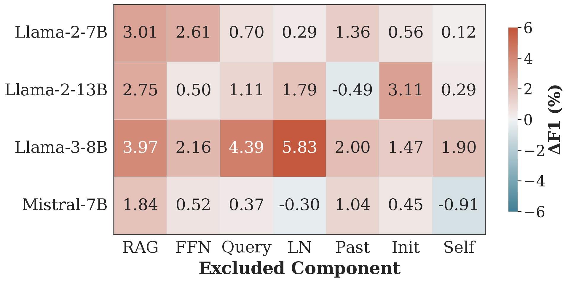
We conduct an ablation study on RAGTruth to validate TPA (Figure 4). The full method generally achieves the best performance. Removing core components like RAG or FFN consistently degrades accuracy (e.g., a 3.01% F1 drop on Llama-2-7B), confirming the importance of the retrievalparameter conflict. Crucially, previously overlooked sources are distinctively vital. For instance, removing LN causes a sharp 5.83% drop on Llama-3-8B. While excluding specific components yields marginal gains in several cases (e.g., Self on Mistral-7B), we retain the complete feature set to maintain a unified framework robust across diverse architectures. We exclude Dolly as its small sample size makes fine-grained feature evaluation unstable.
We apply SHAP analysis to classifiers trained on RAGTruth to validate our design principles. Results for Llama2 are shown in Figure 3, while re- Observation 3: Hallucination fingerprints vary across architectures. Our analysis shows that hallucination signals are model-specific rather than universal. A clear example is LN_NUM: high attribution is a strong hallucination signal in Llama2-7B, but this pattern reverses in Llama2-13B (Figure 3b), where higher values correlate with factuality (negative SHAP values). This reversal suggests that larger models may use LayerNorm differently to regulate output distributions, motivating a learnable, syntax-aware detector.
We introduced TPA to attribute token probability into seven distinct sources. By combining these with syntax-aware features, our framework effectively detects RAG hallucinations and outperforms baselines. Our results show that hallucination signals vary across models. This confirms the need for a learnable approach rather than static heuristics. Future work will proceed in two directions. First, we will extend TPA beyond token-level attribution to phrase-or span-level units so as to improve efficiency. Second, we will explore active mitigation: instead of only diagnosing hallucinations after generation, we will monitor source contributions online and intervene when risky patterns appear, e.g., abnormal reliance on FFN or LN.
Our framework presents three limitations. First, it relies on white-box access to model internals, preventing application to closed-source APIs. Second, the decomposition incurs higher computational overhead than simple scalar probes. Third, our feature engineering depends on external linguistic tools (POS taggers), which may limit generalization to specialized domains like code generation where standard syntax is less defined.
We expand the right-hand side (RHS) of Eq. 8 by substituting the definitions of each term.
First, consider the summation term. By substituting ∆P
This summation forms a telescoping series where adjacent terms cancel:
Now, substituting this result, along with the definitions of ∆P initial and ∆P LN , back into the full RHS expression:
The RHS simplifies exactly to P final (y), which completes the proof.
Proof. We consider the l-th layer of the Transformer. Let h (l-1) ∈ R d be the input hidden state vector at the target position n t . The Multi-Head Attention mechanism computes a residual update ∆h by summing the outputs of H heads:
where u h ∈ R d is the projected output of the h-th head.
The probe function Φ(h, y) computes the probability of the target token y by projecting the hidden state onto the vocabulary logits z ∈ R |V| and applying the Softmax function:
, where
Here, w U,v is the unembedding vector for token v from matrix W U . For brevity, let p y = Φ(h (l-1) , y) denote the probability of the target token at the current state.
We approximate the change in probability, ∆P (l) att , using a first-order Taylor expansion of Φ with respect to h around h (l-1) :
To compute the gradient ∇ h Φ, we apply the chain rule through the logits z v . The partial derivative of the Softmax output p y with respect to any logit z v is given by p y (δ yv -p v ), where δ is the Kronecker delta. The gradient of the logit z v with respect to h is simply w U,v . Thus:
Substituting this gradient back into Eq. ( 18) for a specific head contribution term (denoted as Term h ):
We observe that the dot product w ⊤ U,y • u h is strictly equivalent to the scalar logit contribution ∆z (l) h,y defined in Eq. 10. The factor G (l) = p y (1 -p y ) represents the gradient common to all heads, depending only on the layer input h (l-1) . Therefore, the contribution of head h is dominated by the linear term G (l) • ∆z (l) h,y , subject to the off-target error term E h .
Environment and Models. All experiments were conducted on a computational node equipped with a single NVIDIA A100 (40GB) GPU and 200GB of RAM. Our software stack uses CUDA 12.8, PyTorch 3.10, and HuggingFace Transformers 4.56.1. We evaluate our framework using three Large Language Models: Llama2-7b-chat, Llama2-13b-chat (Touvron et al., 2023), and Llama3-8binstruct (Grattafiori et al., 2024).
Due to GPU memory constraints (40GB), we implement TPA using a sequential prefix-replay procedure (token-by-token), rather than a fully parallel teacher-forced pass. On our hardware, generating the full TPA feature vector for one response takes approximately 20 seconds on average. Since each Initialize v t ∈ R 7 with zeros.
12: L) , y t ) {Contribution from final LayerNorm} 14:
for layer l = 1 to L do 16:
mid , y t ) -Probe(h (l-1) , y t ) 18:
19:
for head h = 1 to H do 20:
Let o h be the output vector of head h.
Compute logit update:
Compute ratio ω h ← exp(∆z h ) j exp(∆z j ) {Logit-based apportionment} Store v t in attribution matrix V. 31: end for 32: return V, Generated Tokens y dataset contains fewer than 3,000 samples, the total feature-extraction cost is on the order of ∼17 GPU-hours per dataset (per evaluated LLM).
Hallucination detection is performed using an ensemble of five XGBoost classifiers; inference is typically well below one second per response, and the total classification cost per dataset is only a few CPU-hours, negligible compared to feature extraction.
For POS tagging, we use spaCy with en_core_web_sm and disable NER.
Feature Extraction and Classifier. For each response, we extract the 7-dimensional attribution vector for every token and aggregate them based on 18 universal POS tags (e.g., NOUN, VERB) defined by the SpaCy library (Honnibal et al., 2020). This results in a fixed-size feature vector (7 × 18 = 126 dimensions) for each sample.
Training and Evaluation Protocols. To ensure fair comparison and statistical robustness, we tailor our training strategies to the data availability of each dataset. We implement strict data isolation to prevent leakage. Crucially, to mitigate the variance inherent in small-data scenarios, we adopt a Multi-Seed Ensemble Strategy. For every experiment, we repeat the entire evaluation process using 5 distinct end for 13: end for 14: 3. Syntax-Aware Aggregation 15: Initialize feature vector f ← ∅. 16: Define set of Universal POS tags P univ . 17: for each POS category c ∈ P univ do 18:
Identify tokens belonging to this category:
// Compute mean attribution profile for this syntactic category f ← Concatenate(f , vc ) 26: end for 27: return f outer random seeds. For each seed, we construct an ensemble of 5 XGBoost classifiers. The final prediction is derived via Hard Voting (majority rule) for binary classification metrics (F1, Recall) and Soft Voting (probability averaging) for AUC. Protocol I: Standard Split (RAGTruth Llama2-7b/13b/Mistral). For datasets with official splits, we utilize the standard training and test sets.
• Optimization: We employ Optuna with a TPE sampler to optimize hyperparameters. We run 50 trials maximizing the F1-score using 5-fold Stratified Cross-Validation on the training set.
• Training: For each of the 5 outer seeds, we train an ensemble of 5 models. Each ensemble member is trained on a distinct 85%/15% split of the training data to facilitate diversity and Early Stopping (patience=50).
• Evaluation: Predictions are aggregated via voting on the held-out test set.
Protocol II: Stratified 20-Fold CV (RAGTruth Llama3-8b). As the Llama3-8b subset lacks a training split, we adopt a Stratified 20-Fold Cross-Validation.
• Optimization: Hyperparameters are optimized via Optuna on the available data prior to the cross-validation loop.
• Training: We iterate through 20 folds. Within each fold, we train the 5-member XGBoost ensemble on the training partition (using diverse internal splits for early stopping).
• Aggregation: Predictions from all folds are concatenated to compute the final performance metrics for each outer seed.
Protocol III: Nested Leave-One-Out CV (Dolly).
Given the limited size of the Dolly dataset (N = 100), we implement a rigorous Nested Leave-One-Out (LOO) Cross-Validation.
• Outer Loop: We iterate 100 times, isolating a single sample for testing in each iteration.
• Inner Loop (Optimization): On the remaining 99 samples, we conduct independent hyperparameter searches using Optuna (50 trials).
• Ensemble Training: For each LOO step, we train 5 XGBoost models on the 99 training samples. To handle class imbalance, we dynamically adjust the scale_pos_weight parameter.
• Inference: The final verdict for the single test sample is determined by the hard vote of the 5 ensemble members. This process is repeated for all 5 outer seeds to verify statistical significance.
Implementation Note regarding Memory Constraints. While TPA is theoretically designed for single-pass parallel execution via teacher forcing, storing the full attention matrices O(T 2 ) and computational graphs for long sequences can be memory-intensive. In our specific experiments, due to GPU memory limitations (NVIDIA A100 40G), we implemented the attribution process sequentially (token-by-token). We emphasize that this implementation is mathematically equivalent to the parallel version due to the causal masking mechanism of Transformer decoders. The choice between serial and parallel implementation represents a trade-off between efficiency and memory usage, without affecting the attribution values or detection performance reported in this paper.
Hyperparameter Search and Best Value Discussion. We utilize the Optuna framework with a Tree-structured Parzen Estimator (TPE) sampler to perform automated hyperparameter tuning.
For each model and data split, we run 50 trials to maximize the F1-score. The comprehensive search space is presented in Table 3. Regarding the best-found values, our analysis reveals that the optimal configuration is highly dependent on the specific LLM and dataset size. We observed a consistent preference for moderate tree depths (4 ≤ max_depth ≤ 6) and stronger regularization (λ ≥ 1.5, γ ≥ 0.2) across most experiments, indicating that preventing overfitting is critical given the high dimensionality of our feature space relative to the dataset size. Conversely, the optimal learning rate varied significantly (0.01 to 0.1) depending on the base model (e.g., Llama-2 vs. Llama-3). Therefore, rather than fixing a single set of hyperparameters, we adopt a dynamic optimization strategy where the best parameters are re-evaluated for each fold and seed. This approach ensures that our reported results reflect the robust performance of the method rather than a specific tuning artifact. 4. ITI (Li et al., 2023) Detecting hallucination based on the hidden layer activations of LLMs.
-
Ragtruth Prompt (Niu et al., 2024) Provdes prompts for a LLM-as-judge to detect hallucination in RAG setting.
-
ChainPoll (Friel and Sanyal, 2023) Provdes prompts for a LLM-as-judge to detect hallucination in RAG setting.
-
RAGAS (Es et al., 2024) It use a LLM to split the response into a set of statements and verify each statement is supported by the retrieved documents. If any statement is not supported, the response is considered hallucinated.
-
Trulens(TrueLens, 2024) Evaluating the overlap between the retrieved documents and the generated response to detect hallucination by a LLM. 9. P(True) (Kadavath et al., 2022) The paper detects hallucinations by having the model estimate the probability that its own generated answer is correct, based on the key assumption that it is often easier for a model to recognize a correct answer than to generate one.
-
SelfCheckGPT (Manakul et al., 2023) Self-CheckGPT detects hallucinations by checking for informational consistency across multiple stochastically sampled responses, based on the assumption that factual knowledge leads to consistent statements while hallucinations lead to divergent and contradictory ones.
-
LN-Entropy (Malinin and Gales, 2021) This paper detects hallucinations by quantifying knowledge uncertainty, which it measures primarily with a novel metric called Reverse Mutual Information that captures the disagreement across an ensemble’s predictions, with high RMI indicating a likely hallucination.
-
Energy (Liu et al., 2020) This paper detects hallucinations by using an energy score, derived directly from the model’s logits, as a more reliable uncertainty measure than softmax confidence to identify out-of-distribution inputs that cause the model to hallucinate.
-
Focus (Zhang et al., 2023) This paper detects hallucinations by calculating an uncertainty score focused on keywords, and then refines it by propagating penalties from unreliable context via attention and correcting token probabilities using entity types and inverse document frequency to mitigate both overconfidence and underconfidence.
-
Perplexity (Ren et al., 2023)
-
Head-wise Attribution. Once ∆P (l)
att is obtained, we apportion it to individual heads based on their contribution to the target logit.
• Mechanism: This attribution requires projecting the target token vector w U,y back into the hidden state space using the layer’s output projection matrix W
O ∈ R d×d .
•
Step Complexity: The calculation proceeds in two sub-steps:
- Projection: We compute the projected target vector g = (W
O is a d × d matrix, this matrix-vector multiplication costs O(d 2 ). 2. Assignment: We distribute the contribution to H heads by performing dot products between the head outputs o h and the corresponding segments of g. For H heads, this sums to O(d).
•
Attention to Input Sources. Finally, we map head contributions to the four sources by aggregating attention weights A ∈ R H×|s|×|s| . This involves two distinct sub-steps for each generated token at step t within a single layer:
•
Step 1: Summation. For each head h, we sum the attention weights corresponding to specific source indices (e.g., I RAG ):
This requires iterating over the causal range up to n t . For H heads, the cost is O(H • n t ).
•
Step 2: Normalization & Weighting. We calculate the final source contribution by weighting the head contributions:
This involves scalar operations proportional to the number of heads H. Cost: O(H).
• Stage Complexity: The summation step (O(H • n t )) dominates. We sum this cost across all L layers, and then accumulate over the generation steps t = 1 to T . The calculation is
Overall Efficiency. The total computational cost is the sum of these three stages: (Ren et al., 2023) 0.5091 0.5190 0.6749 0.5091 0.5190 0.6749 0.6235 0.6537 0.6778 LN-Entropy (Malinin and Gales, 2021) 0.5912 0.5383 0.6655 0.5912 0.5383 0.6655 0.7021 0.5596 0.6282 Energy (Liu et al., 2020) 0.5619 0.5057 0.6657 0.5619 0.5057 0.6657 0.5959 0.5514 0.6720 Focus (Zhang et al., 2023) 0.6233 0.5309 0.6622 0.7888 0.6173 0.6977 0.6378 0.6688 0.6879 Prompt (Niu et al., 2024) -0.7200 0.6720 -0.7000 0.6899 -0.4403 0.5691 ChainPoll (Friel and Sanyal, 2023) 0.6738 0.7832 0.7066 0.7414 0.7874 0.7342 0.6687 0.4486 0.5813 RAGAS (Es et al., 2024) 0.7290 0.6327 0.6667 0.7541 0.6763 0.6747 0.6776 0.3909 0.5094 Trulens (TrueLens, 2024) 0.6510 0.6814 0.6567 0.7073 0.7729 0.6867 0.6464 0.3909 0.5053 RefCheck (Hu et al., 2024) 0.6912 0.6280 0.6736 0.7857 0.6800 0.7023 0.6014 0.3580 0.4628 P(True) (Kadavath et al., 2022) 0.7093 0.5194 0.5313 0.7998 0.5980 0.7032 0.6323 0.7083 0.6835 EigenScore (Chen et al., 2024) 0.6045 0.7469 0.6682 0.6640 0.6715 0.6637 0.6497 0.7078 0.6745 SEP (Han et al., 2024) 0.7143 0.7477 0.6627 0.8089 0.6580 0.7159 0.7004 0.7333 0.6915 SAPLMA (Azaria and Mitchell, 2023) 0.7037 0.5091 0.6726 0.8029 0.5053 0.6529 0.7092 0.5432 0.6718 ITI (Li et al., 2023) 0.7161 0.5416 0.6745 0.8051 0.5519 0.6838 0.6534 0.6850 0.6933 ReDeEP (Sun et al., 2025) 0.7458 0.8097 0.7190 0.8244 0.7198 0.7587 0.7285 0.7819 0.6947 TSV (Park et al., 2025) 0 (Ren et al., 2023) 0.2728 0.7719 0.7097 0.2728 0.7719 0.7097 0.1095 0.3902 0.4571 LN-Entropy (Malinin and Gales, 2021) 0.2904 0.7368 0.6772 0.2904 0.7368 0.6772 0.1150 0.5365 0.5301 Energy (Liu et al., 2020) 0.2179 0.6316 0.6261 0.2179 0.6316 0.6261 -0.0678 0.4047 0.4440 Focus (Zhang et al., 2023) 0.3174 0.5593 0.6534 0.1643 0.7333 0.6168 0.1266 0.6918 0.6874 Prompt (Niu et al., 2024) -0.3965 0.5476 -0.4182 0.5823 -0.3902 0.5000 ChainPoll (Friel and Sanyal, 2023) 0.3502 0.4138 0.5581 0.4758 0.4364 0.6000 0.2691 0.3415 0.4516 RAGAS (Es et al., 2024) 0.2877 0.5345 0.6392 0.2840 0.4182 0.5476 0.3628 0.8000 0.5246 Trulens (TrueLens, 2024) 0.3198 0.5517 0.6667 0.2565 0.3818 0.4941 0.3352 0.3659 0.5172 RefCheck (Hu et al., 2024) 0.2494 0.3966 0.5412 0.2869 0.2545 0.3944 -0.0089 0.1951 0.2759 P(True) (Kadavath et al., 2022) 0.1987 0.6350 0.6509 0.2009 0.6180 0.5739 0.3472 0.5707 0.6573 EigenScore (Chen et al., 2024) 0.2428 0.7500 0.7241 0.2948 0.8181 0.7200 0.2065 0.7142 0.5952 SEP (Han et al., 2024) 0.2605 0.6216 0.7023 0.2823 0.6545 0.6923 0.0639 0.6829 0.6829 SAPLMA (Azaria and Mitchell, 2023) 0.0179 0.5714 0.7179 0.2006 0.6000 0.6923 -0.0327 0.4040 0.5714 ITI (Li et al., 2023) 0.0442 0.5816 0.6281 0.0646 0.5385 0.6712 0.0024 0.3091 0.4250 ReDeEP (Sun et al., 2025) 0.5136 0.8245 0.7833 0.5842 0.8518 0.7603 0.3652 0.8392 0.7100 TSV (Park et al., 2025) 0
† 0.9741 † 0.8075 † 0.7608 † 0.6561 0.7529 † Table 1: Results on RAGTruth and Dolly (AC). TPA results are averaged over 5 random seeds. The dagger symbol † indicates statistically significant improvement (p < 0.05) over the strongest baseline. Bold values indicate the best performance and underlined values indicate the second-best. Full results in Appendix.
This content is AI-processed based on open access ArXiv data.