InverseCrafter: Efficient Video ReCapture as a Latent Domain Inverse Problem
📝 Original Info
- Title: InverseCrafter: Efficient Video ReCapture as a Latent Domain Inverse Problem
- ArXiv ID: 2512.05672
- Date: 2025-12-05
- Authors: Yeobin Hong, Suhyeon Lee, Hyungjin Chung, Jong Chul Ye
📝 Abstract
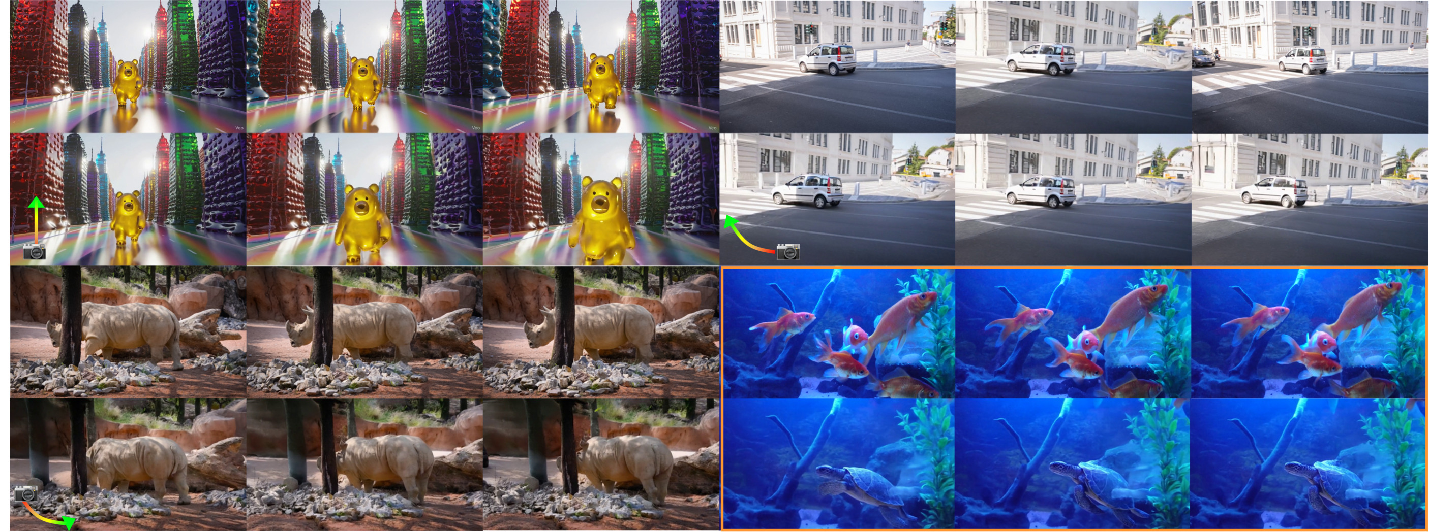
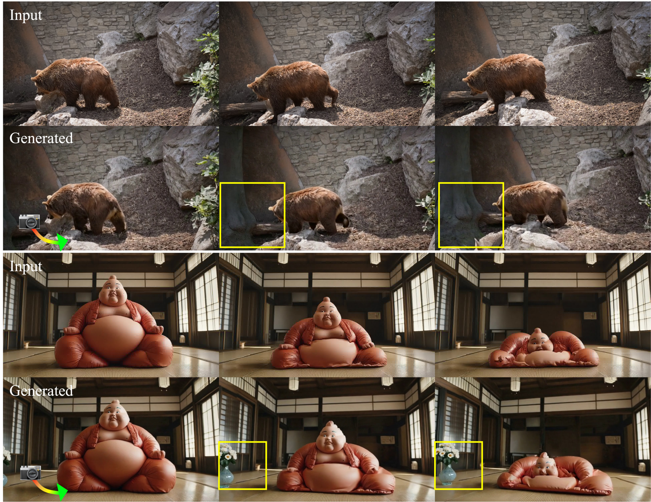
Figure 1 . Representative video on camera control ("zoom in," "arc left," "arc right") and inpainting with editing ("goldfish" to "turtle").📄 Full Content
One promising branch of research that has emerged to address the challenge for 4D synthesis is the framing of the problem as a video-to-video translation task: given a user input video, synthesize novel views over time while following a target camera trajectory (e.g., camera control). A line of work fine-tunes VDMs to condition on prospective cameras [3,50,55], which requires large-scale 4D datasets and still generalizes poorly to unseen camera trajectories. Another branch [15,42,56,61] reframes the task as 3D-aware inpainting (see Fig. 2(a-1)). These methods leverage 3D reconstruction priors (e.g., depth estimation or point tracking) to first generate large-scale, pseudo-annotated datasets and then fine-tune the VDM to inpaint the occluded regions. This training process often creates a strong dependency on the specific 3D reconstruction model used during training. Furthermore, some methods additionally modify the VDM architecture to augment the VDM architecture (e.g., adding new attention blocks [56,61]), substantially increasing inference latency. Fine-tuning also induces overfitting and catastrophic forgetting, degrading the pretrained model’s general text-to-video generation capabilities and preventing it from functioning as a versatile generative prior. Alternatively, per-video optimization approaches [21] avoid large-scale retraining as shown in Fig. 2(a-2), but they overfit to individual scenes and fail to generalize.
A promising, training-free alternative formulates 4D video generation as an inverse problem, where the warped video serves as a measurement. However, adapting diffusion inverse solvers from the image domain to video inpainting presents several challenges. For instance, NVS-Solver [60] in Fig. 2 (a-3) utilizes Diffusion Posterior Sampling (DPS) [11]. Applying computationally expensive backpropagation [11] required for DPS through the VDM at every sampling step is impractical. Conversely, backpropagation-free solvers [12,52] are often restricted to (near) linear inverse problems, making them unsuitable for this non-linear inpainting task 1 . Furthermore, a critical flaw plagues nearly all recent video inpainting methods [21,38,60,61] as they naively resize pixel space masks to the latent domain, incorrectly assuming that spatio-temporal features and relationships are preserved in the latent domain.
To address this clear gap, we present InverseCrafter, which introduces a principled mechanism to project pixel space masks (m) into a high-fidelity continuous latent mask (h) (see Fig. 2(b)). This core contribution enables the adaptation of a computationally efficient inverse solver that operates entirely within the VDM’s latent space. We present two highly effective options -a learned mask encoder or a training-free projection. Both approaches produce a high-fidelity latent mask that respects the VAE’s channeldependent representations, a critical step that prior work overlooks. By performing guidance entirely in the latent space, our method avoids the costly bottleneck of VAE en- 1 The problem is non-linear in the latent space due to the VAE encoder. coding/decoding and backpropagation at every sampling step, drastically reducing computation time. Our main contributions are summarized as follows:
• We introduce a novel InverseCrafter that formulates controllable 4D video generation as an inverse problem, enabling the use of pre-trained VDMs without fine-tuning. • We propose a general and efficient backpropagation-free inpainting inverse solver that operates entirely in the latent space, supported by a continuous mask representation. • Our framework achieves near-zero additional inference cost over standard diffusion inference while producing high-fidelity, spatio-temporally coherent videos.
Video Inpainting for 4D Generation. Recent works [15,42,56,61] frame 4D video-to-video translation task as an inpainting problem by generating conditional inputs using a 3D reconstruction model and then fine-tuning the VDM to inpaint the occluded regions. Other works have attempted to solve the video re-angling task using training-free methods by adapting diffusion inverse solvers. For instance, NVS-Solver [60] employed diffusion Posterior Sampling (DPS).
To mitigate the prohibitive computational cost associated with VAE decoding and gradient computation at each step, NVS-Solver performs its operations directly in the latent space. Unfortunately, [60] struggles with generalization and stability, as it relies on hand-crafted hyperparameters for specific VDM architectures [6]. On the other hand, Zero4D [38] formulates the 4D video generation as a video interpolation problem in the latent domain by employing mask resizing and a subsequent mask-based interpolation between the generated output and the measurement. A critical limitation of these approaches is their reliance on models like Stable Video Diffusion (SVD) [6], whose VAE performs spatial compression only. Both methods project the degradation operator (pixel space mask) into the latent space via simple average pooling over the spatial dimensions. This challenge of correctly formulating the measurement and masking operation in the latent space is a common, unaddressed issue. Heuristics to spatially compressing the mask are inherited from the image diffusion literature, where inverse solvers either decode to pixel space or apply an arbitrarily resized masking operator in the latent space. The problem of binary resizing is significantly exacerbated when it comes to modern Video Diffusion Models (VDMs). Since modern VDMs utilize 3D VAEs for spatio-temporal compression, mapping a 2D pixel space mask to a 3D latent space is ill-defined.
Diffusion Models for Inverse Problems. Consider the following forward problem:
where A is the forward mapping and n is additive noise. Then, the goal of the inverse problem is to retrieve x from the corrupted y. While diffusion models are trained to sample from p(x), diffusion model-based inverse problem solvers can guide the generation process during inference time to perform approximate posterior sampling x ∼ p(x|y) [14]. Notably, all zero-shot methods aim to minimize the data consistency ∥y-A(x)∥ 2 during the sampling process. For pixelbased diffusion models, this is relatively straightforward, as the estimates during generation remain in the pixel space. In contrast, using these solvers with LDMs-which dominate modern literature-requires special treatment. Most solvers that operate in the latent space [13,24,44,47] first decode the estimated latent to the pixel space, and measure the consistency in the decoded pixel space. The process of correcting the latent further induces approximation errors and heavy computation, often leading to blurry samples. Recently, SILO [41] proposed to mitigate this gap by training a network to estimate the latent forward model, so that one can bypass the need for decoding to pixel space during sampling, leading to competitive results in standard image restoration tasks. Motivated by SILO, in this work, we devise ways to solve the dynamic NVS task purely in the latent space.
Problem Formulation. To solve the inverse problem of novel view synthesis, we must formulate the measurement y based on 3D geometric constraints. This requires projecting the source video into a target camera view. First, we establish a 3D representation of the scene. We process the source video x 1:F frame-by-frame using a pre-trained monocular depth estimation network [19] to acquire a perframe estimated depth map D1:F . Next, for each frame i, we unproject the 2D pixel coordinates (from the image x i ) into a 3D point cloud P i using the estimated depth Di and an intrinsic camera matrix K. This back-projection function is denoted Π -1 :
Once the scene is represented in 3D, we can render it from a new perspective. The 3D point cloud P i is transformed into the target camera’s coordinate system using a relative transformation matrix T i . These transformed points are then projected back into a 2D image y i using the forward projection function Π:
The warped video y := y 1:F represents the pixel space measurement, which contains occlusions from the 3D warping process, which can be succinctly written as
where ⊙ denotes the element-wise product and N = F HW is the pixel space resolution, and m refers to a binary mask indicating the occlusion from the 3D warping process.
Recent video diffusion models [51,59] introduce 3D VAEs that perform spatiotemporal compression, creating the need to reformulate the pixel-domain forward model in Eq. ( 4) in the latent domain. These architectures map pixel resolutions (F, H, W ) to latent resolutions (f, h, w), where spatial dimensions are reduced by a factor of 8, similar to image VAEs, and the temporal dimension is commonly compressed by a factor of 4. Inference-time image inpainting methods for latent diffusion models [22,23] typically construct latent masks by projecting pixel-space masks into the latent space via an 8× downsampling with nearest-neighbor interpolation. However, the additional temporal compression in video models necessitates special consideration beyond these image-based techniques.
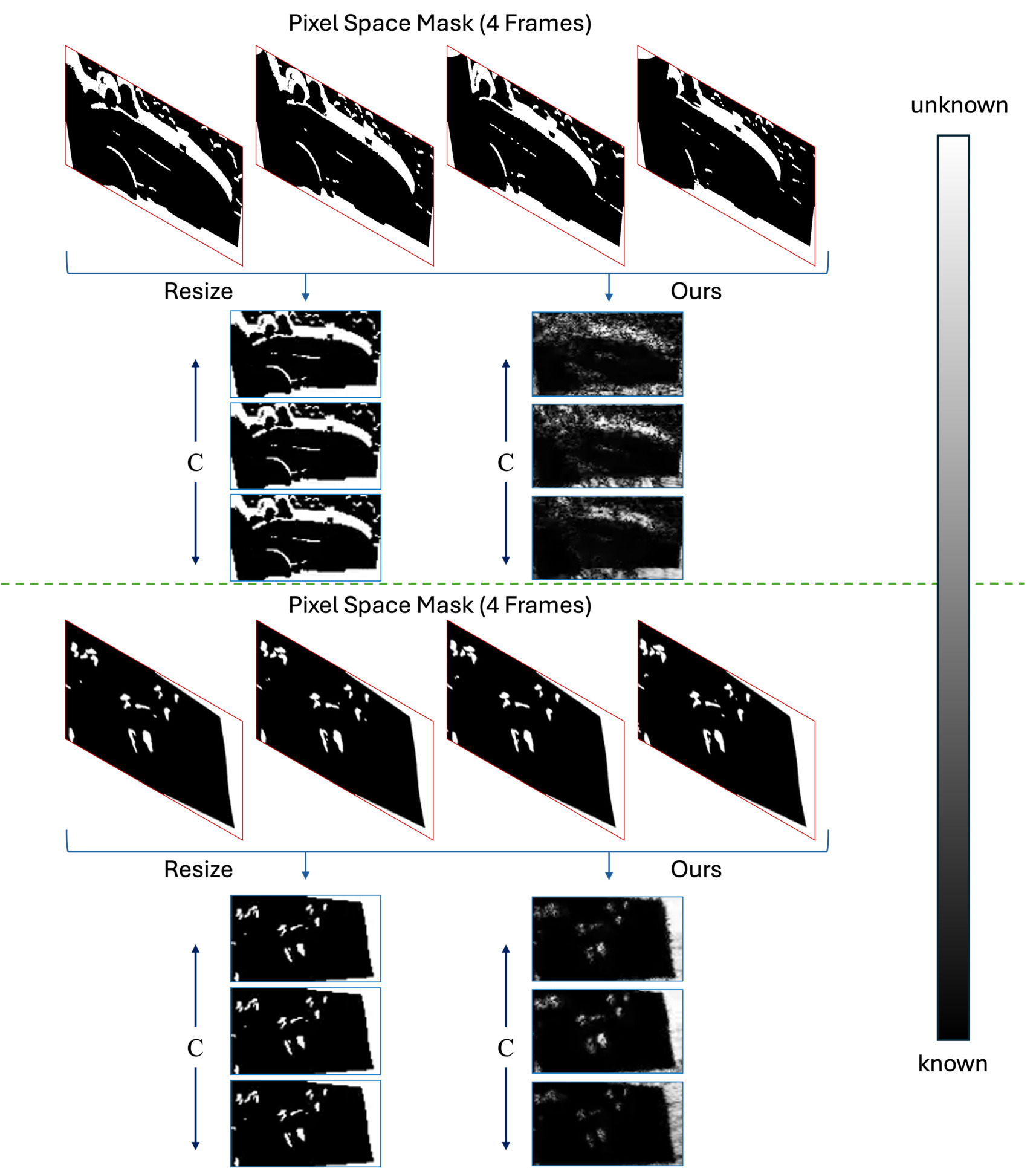
Nevertheless, recent video inpainting methods that operate directly in the latent domain [21,56,61] largely adopt direct spatiotemporal projection (i.e., spatiotemporal interpolation) as a naive extension of image-based approaches. This practice relies on several problematic assumptions. First, it implicitly assumes that spatial structures in pixel space are preserved under the non-linear VAE encoder, which is generally false. Second, it treats the latent mask as uniform across channels, despite the fact that latent channels encode highly heterogeneous feature representations, as illustrated in Fig. 2(a) (visualizations in Appendix C.1). Third, some methods [21,61] adopt an overly conservative temporal rule: a latent region is marked as “known” only if its corresponding pixel region is visible in all frames within its temporal group. This strategy becomes a major bottleneck for videos with fast motion. If an object appears in only a subset of frames due to rapid movement or partial occlusion, the entire corresponding latent region is marked as “unknown,” which forces unnecessary inpainting and increases reliance on the generative model, as shown in Fig. 8(a).
Generating Continuous Mask. To address the mask projection inconsistencies outlined previously, we propose learning a lightweight neural network, dubbed the mask encoder P ϕ (•) : R N → R C×M , where C denotes the number of latent channels and M = f hw represents the latent-space resolution, to compute an accurate latent-space mask that takes in as input the pixel measurement y and outputs a continuous mask that can be applied linearly to the latent z, with the same Hadamard product operation as in Eq. (4).
Our training target is derived from the observation that autoencoders are effective at reconstructing degraded data [41]. We define this ground-truth latent mask, h ∈ R C×M , as the normalized difference between the latent encoding of the clean video, E(x), and the latent encoding of the masked video, E(m ⊙ x):
where f stands for normalization using an activation function, scaling the latent difference to a [0, 1] range. However, a primary challenge is obtaining training pairs, as for generating warped videos (Eq. ( 3)), the corresponding “ground truth” video x is not available. To resolve this, we employ a double-reprojection strategy from [61] to synthesize the correctly masked counterpart m ⊙ x from the clean video x, which provides the necessary pair to compute h.
The mask encoder is then trained to predict this groundtruth latent mask directly from the pixel space mask with a combination of the L1 loss and the Structural Similarity Index Measure (SSIM) [53] loss:
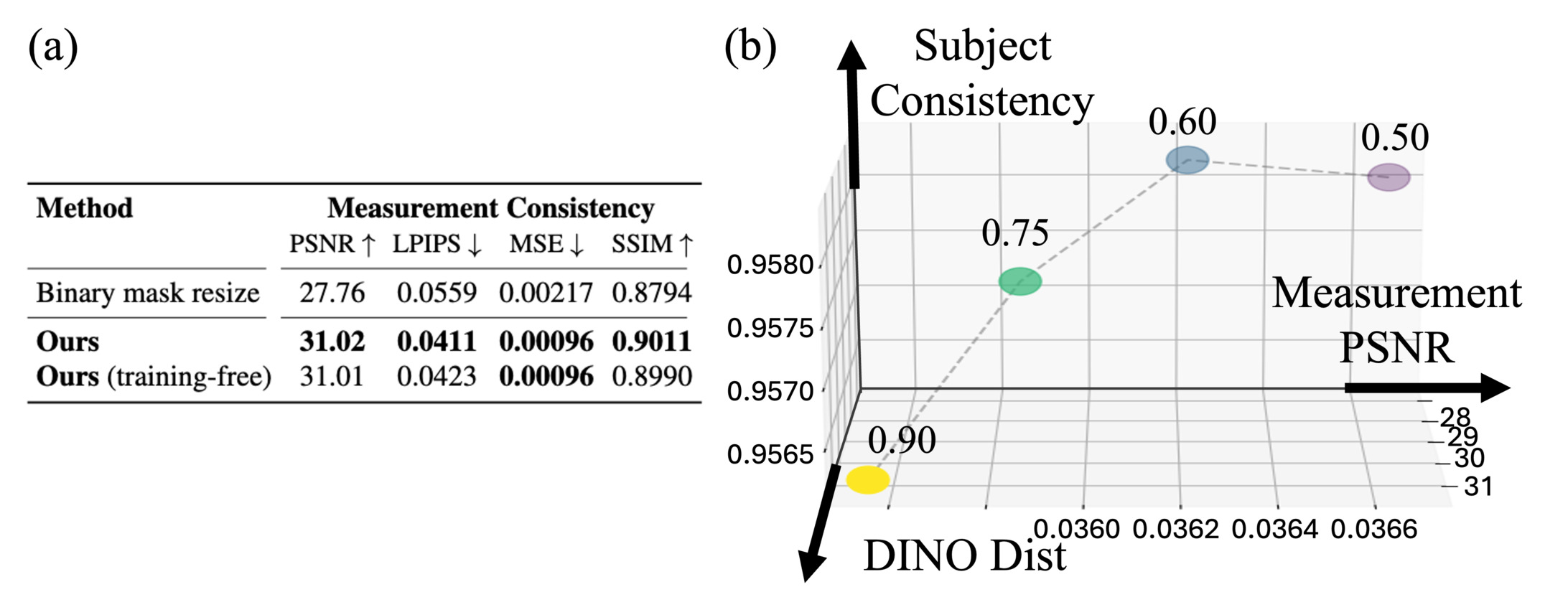
Unlike naive mask resizing, which generates a singlechannel binary mask that is uniformly broadcast across all C latent channels (ignoring their distinct feature representations), our mask encoder outputs a continuous, C-channel mask. This high-fidelity representation better captures the mask’s influence across the latent features, leading to improved VAE reconstruction and superior measurement consistency in final generated outputs, as detailed in Fig. 7-(a).
Furthermore, for tasks such as video inpainting with editing (detailed in Section 4.3.2), where a valid ground-truth latent mask h is available at inference time, P ϕ can be bypassed. In addition, we empirically found that a training-free strategy is also possible for the video camera control task. Specifically, we compute an approximate latent mask onthe-fly as h = f(E(x src ) -E(m warp ⊙ x src )). While the trained P ϕ is optimized to achieve superior VAE reconstruction and measurement consistency (as shown in Table 1 and Fig. 7
end if 20: end for 21: x tgt ← D(z 0 ) latent mask generation. Alg. 1 summarizes the full pipeline.
DDS for Latent Inpainting with Continuous Masks. To align with the latent diffusion model, we encode the pixel space measurement into the latent space using the VAE encoder E. Then, under our noiseless linear setting of Eq. ( 4), the inverse problem in the pixel domain transforms to an inverse problem in the latent space, i.e.
Notice that the design of our mask encoder P ϕ is different from that of [41]. The operator encoder used in [41] acts non-linearly on the encoded latent z to produce the latent measurement w, whereas our mask encoder produces a continuous linear mask h, which can be applied linearly with a Hadamard product. Thanks to such a design choice, we are free from selecting any diffusion model-based inverse problem solvers, even the ones that are specialized for solving linear inverse problems in the pixel space. Among them, we propose to leverage DDS [12]. Namely, the data consistency step of DDS solves the following proximal optimization problem :
which is followed by the ODE solver. Here, ẑ0|t := E[z 0 |z t ] is the estimated posterior mean with the flow model v θ , and γ is a hyper-parameter that controls the proximal regularization. Following [12], we solve Eq. ( 8) using conjugate gradient (CG) iterations. Specifically, let H := diag(h). Then, Eq. ( 8) can be solved with CG(I + γH ⊤ H, ẑ0|t + γH ⊤ w, ẑ0|t , K) with K iterations.
Task. We evaluate our method on two major video inpainting tasks: video camera control and text-guided video inpainting. Our primary focus is the video camera control task, for which we use 1,000 videos and corresponding captions from the UltraVideo dataset [58]. We sample one of the six target camera trajectories for each video, where the target trajectories are selected following the work in [21]. For text-guided video inpainting, we apply our proposed video inpainting method to replace objects in the video, guided by target text prompts and source object masks. This evaluation is conducted on 20 videos from the DAVIS [39] dataset, along with all available foreground masks. For each video, we generate five target editing prompts using GPT-5-mini [36], while the corresponding source captions used for prompt construction are obtained using BLIP-2 [31].
Evaulation. For the video camera control tasks, we assess performance using a comprehensive set of metrics: measurement consistency metrics -measurement PSNR, LPIPS, SSIM, source consistency metrics -DINO distance [10], Fréchet Video Distance (FVD), and general video quality metrics -subject consistency, temporal flickering, motion smoothness, and overall consistency from VBench [20]. The measurement consistency metric was compared by the warped video, frame by frame. DINO and FVD were calculated by reference to the source video datasets. For video inpainting tasks, we additionally evaluate the generated videos with the editing text-alignment metrics: VLM (see appendix B.2 for details), Clip Score [40] and Pick Score [25].
Training. We train our model on the VidSTG [62] dataset.
For each of the 7,750 videos in the dataset, we generate 6 double-reprojection datasets from the selected camera trajectories, resulting in a total of 46,500 training samples. We utilize DepthCrafter [19] for monocular depth estimation. Our model architecture is based on the Wan2.1 VAE, which we modify to create a lightweight model by reducing the channel dimension from 96 to 16, resulting in 1.5M parameters. The model is trained at a fixed resolution of 240×416. We employ the AdamW optimizer [35] with a learning rate of 1 × 10 -4 and a weight decay of 3 × 10 -2 . Training is conducted with a total batch size of 16, distributed as 4 samples per GPU across 4 GPUs, completed in 1 day.
Inference. In this paper, we use Wan2.1-Fun-V1.1-1.3B-InP [51] at a resolution of 480×832, a pre-trained imageto-video flow-based model for the main experiments. For encoding masked videos during training or inference, as in [21], we infill the masked region to minimize the traininference following gap [45]. We use [19] for all trainingfree methods and TrajectoryCrafter for fair comparison to generate a depth map for each frame. Compute Resources. All training and inference experiments are conducted using NVIDIA RTX A6000 GPUs (48GB VRAM). A detailed runtime analysis is provided in Table 1.
Table 1 reports results on the video camera control task compared to major baselines. Despite requiring neither additional training data nor VDM fine-tuning, and adding virtually no overhead beyond standard diffusion inference, our method achieves performance comparable to or better than existing approaches. Furthermore, it delivers consistently strong results across source consistency, measurement consistency, and overall video quality, indicating reliable behavior in practical video generation settings. Notably, methods that depend on large-scale VDM training or heavy gradient-based optimization incur significant computational cost, whereas our approach attains competitive or superior performance while remaining entirely training-free and lightweight.
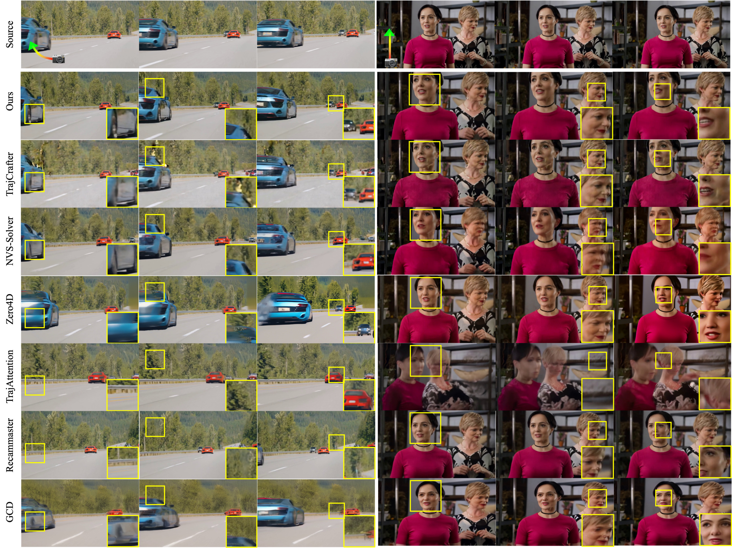
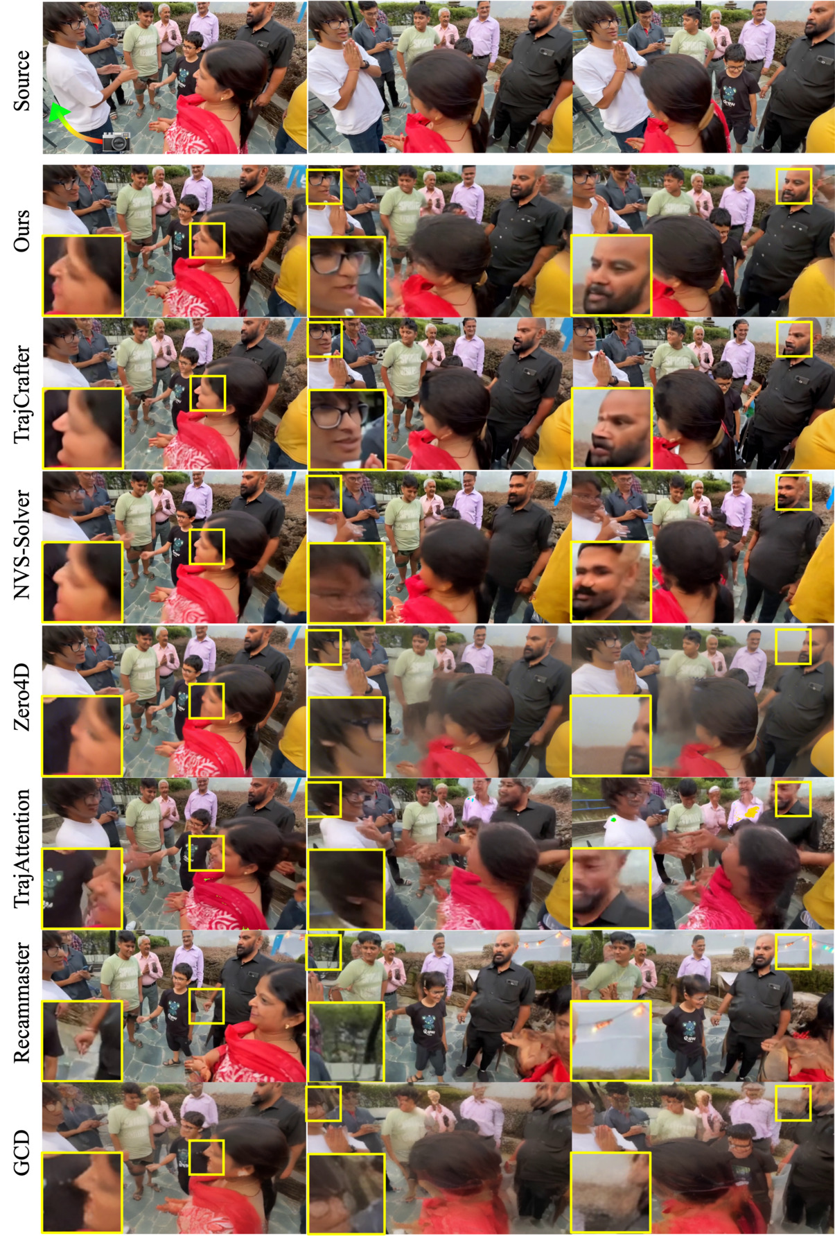
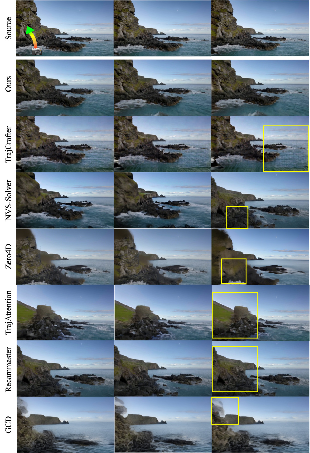
The qualitative comparisons in Fig. 5 further show that baseline training-based or backpropagation methods (Tra-jectoryCrafter, NVS-Solver (post), TrajectoryAttention, Re-CamMaster) generate artifacts (e.g. in the trees) or fail to faithfully preserve the source video’s content (e.g. background car and women’s faces). Backpropagation-free methods (NVS-Solver (dgs), Zero4D) fail to capture the video’s motion (e.g. background car), generate boundary artifacts, or result in highly saturated videos. On the other hand, our method maintains higher fidelity to the source while preserving visual coherence, demonstrating the practical benefit and reliability of our efficient, training-free formulation.
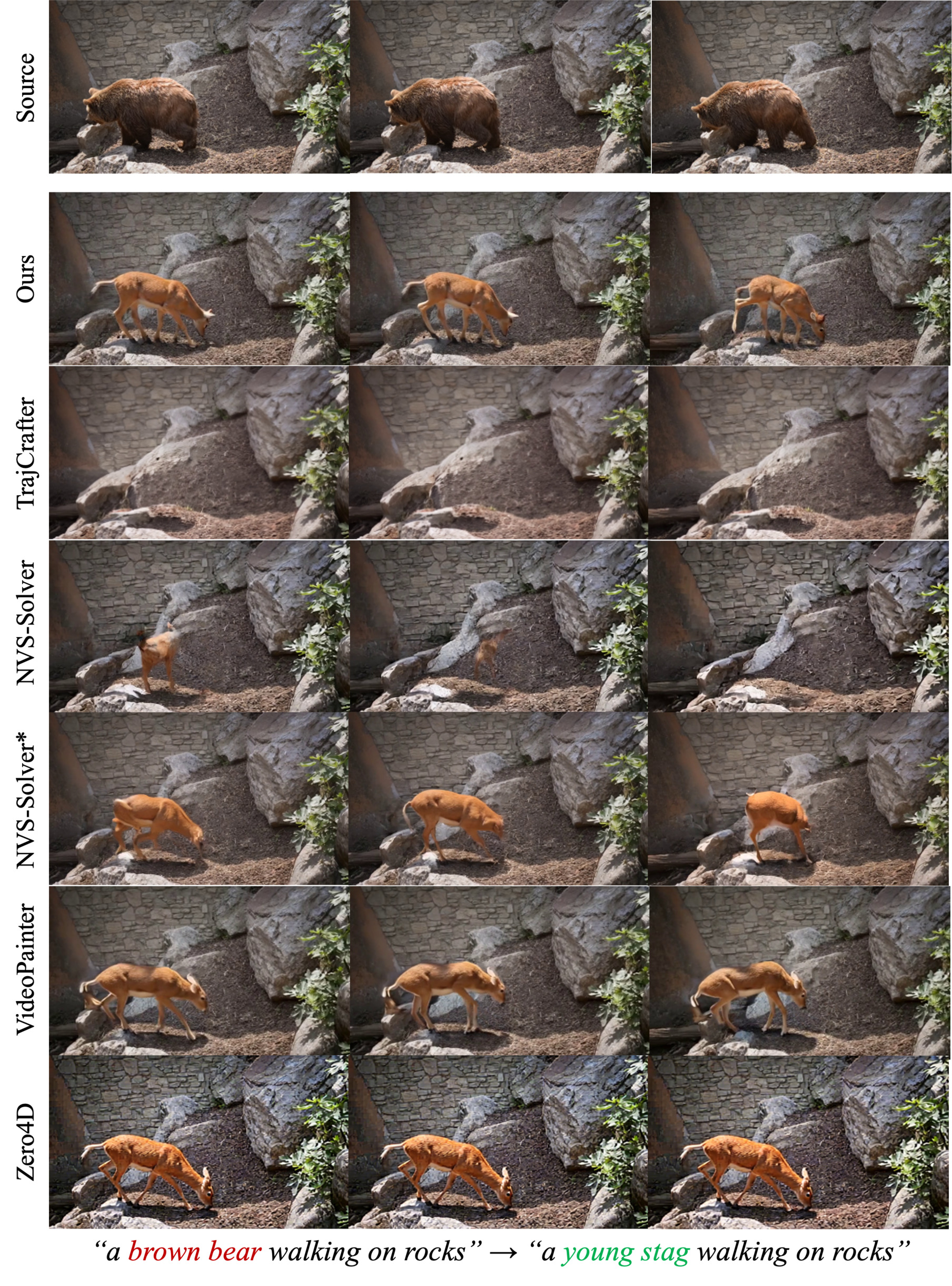
Furthermore, Fig. 4 highlights our method’s effectiveness in text-conditioned novel content generation. By leveraging the pre-trained VDM as a generative prior, our approach maintains superior semantic alignment, successfully synthesizing contextually consistent content even during complex geometric manipulation.
As first frame conditioning is essential for I2V models, we provide first-frame conditioning input for training-free methods (NVS-Solver, Zero4D) and VideoPainter, which also utilizes an I2V model. We obtain the first-frame conditioning input using an off-the-shelf image inpainting model [30].
The proposed method outperforms the baselines in source distribution and video text alignment metrics in Table 2. While Zero4D [38] outperforms image based text alignment metrics, this comes from the fact that output video of Zero4D is nearly static as shown in Fig. 6. In the second example, In-verseCrafter uniquely generates the volleyball in the masked region, while also matching the measurement, whereas all baselines fail to generate regarding the target text. In both examples, NVS-Solver (post) deviates a lot from the measurement, NVS-Solver (dgs) and VideoPainter generates boundary artifacts and inferior results. This implies that our method can be used as a general inpainting inverse solver, integrating text descriptions by fully utilizing the pre-trained model’s generative prior.
Fig. 7-(a) compares our continuous latent mask with conventional binary mask resizing using ×8 nearest-neighbor spatially and logical AND downsampling temporally. Our method shows better measurement consistency, where using the trained P ϕ shows the best reconstruction, following our training-free version. Fig. 8-(a) shows qualitative comparison of the masking strategies. Reconstructed measurement of binary downsampling doesn’t align with the original measurement due to the conservative masking strategy, failing to properly reconstruct the mask in sequences with fast motion. Conversely, our method generates a consistent continuous mask, thereby preserving the fidelity of the measurement. Fig. 8-(b) compares our method with conventional pixel space DDS as in prior methods [27,28], which requires additional VAE encoding and decoding at every timestep, a costly bottleneck that our method entirely avoids. Furthermore, as highlighted by the insets, pixel space Conjugate Gradient introduces severe color and textural inconsistencies. In contrast, our proposed method enables seamless integration with measurement without these artifacts. We set Γ as Γ = {t|t ≥ 1 -α}. When using a larger α (i.e., applying the measurement consistency step earlier in the diffusion process), the result exhibits stronger consistency with the source measurement and improved content faithfulness. In contrast, a smaller α delays the measurement consistency update to later diffusion steps, emphasizing the model’s generative prior and producing more visually refined outputs. This demonstrates that α effectively controls the balance between the diffusion prior and measurement constraints during posterior sampling, where we observe that setting α = 0.6 consistently achieves a favorable balance between semantic alignment and structure preservation.
In this paper, we presented a novel and efficient framework for novel-view video generation by casting the task as an inverse problem fully defined in the latent space. The core of our method is a principled mechanism for projecting pixelspace masks into continuous, multi-channel latent representations. Our experiments demonstrate that this approach achieves superior measurement consistency while preserv- ing comparable generation quality in the camera control task. We further show its effectiveness as a general-purpose video inpainting solver for editing tasks. Overall, our framework offers a versatile and lightweight solution for controllable 4D video synthesis, eliminating the need for computationally expensive VDM fine-tuning and incurring no additional inference-time overhead.
Limitations and future work. Although our solver is efficient, its speed is limited by multi-step diffusion sampling process. Our method inherits the pre-trained VDM’s inherent biases. The initial warping stage is a major source of artifacts due to its dependence on potentially inaccurate monocular depth estimates. Finally, while our trainingfree mask computation is model-agnostic, the learned mask encoder is tailored to a specific VAE architecture.
Backpropagation-Free Solvers To address the high computational cost, a second line of work seeks to avoid this backpropagation. Decomposed Diffusion Sampling (DDS) [12], for example, synergistically combines diffusion sampling with classical optimization methods. For linear inverse problems, this update is equivalent to solving a proximal optimization problem:
which can be solved efficiently using a small number of Conjugate Gradient (CG) steps. This approach eliminates the need to compute the costly Manifold-Constrained Gradient (MCG), resulting in dramatic accelerations.
Early efforts to imbue VDMs with precise camera control involved modifying the model architecture or training process. This included training external modules to inject conditioning information such as camera parameters [16,32], conditioning the model on explicit geometric representations like Plücker embeddings [1,55], or inflating the attention mechanisms of the base VDM [2,48,54,57].
Video-to-Video Translation for Camera Control More recently, the problem has been effectively framed as a video-tovideo translation task. The first and most common direction involves fine-tuning a pre-trained VDM. This includes methods that train the model to directly accept camera parameters as input conditions [3,50,55], or methods that tries to solve a 3D-aware inpainting problem [15,21,56]. These methods warp the source video according to the target trajectory and then fine-tune the VDM to realistically inpaint the resulting occluded or disoccluded regions. The second, training-free methods adapt pre-trained VDMs as powerful generative priors, typically by reformulating the task as an inverse problem that can be solved at inference time [38,60]. Our work builds upon this paradigm by developing a more efficient and robust latent-space solver for this task.
The Text-guided Inpainting dataset consists of video clips, target masks, source prompts, and target prompts. We selected 20 videos and target mask pairs from the DAVIS [9] dataset. In each pair, the foreground in the mask is treated as the inpainting target. For source prompt generation, we used the BLIP-2 [31] model to generate a caption describing the middle frame of each video. The target prompts were then generated using the gpt-5-mini-2025-08-07 [36] model, which took the source prompt as input along with the following instruction prompt (Fig. 9). A total of five target prompts were generated for each video, resulting in a dataset containing 125 samples.
For the quantitative comparison, we evaluate following metrics following the evaluation code3 4 5 6 : 1. Measurement PSNR : We compute the PSNR by excluding the masked region, resulting in the measurement PSNR. 2. Measurement LPIPS : We measure the LPIPS [7], which is defined as distance between feature maps of pre-trained VGG network, by excluding the masked region. 3. Measurement SSIM : We compute the structural similarity [53] by excluding the masked region. 4. DINO distance : We evaluate source distribution consistency by computing the average cosine distance between DINO-ViT [10] features extracted from the generated video and the source video. 5. FVD : We report the Fréchet Video Distance (FVD) [49] to assess the overall quality and temporal coherence of the generated videos, using features from a pre-trained I3D network. 6. VBench: We calculate subject consistency, temporal flickering, motion smoothness for Quality Score and overall consistency for Semantic Score, calculate the Total Score based on the metric weights & normalization method in VBench. 7. CLIP-score : We report the similarity between features embedded by pre-trained CLIP [40] 7 image encoder and text encoder.
Require: A, y, x 0 , M 1: r 0 ← b -Ax 0 2: p 0 ← b 0 3: for i = 0 : K -1 do do 4:
x k+1 ← x k + α k p k 6:
r k+1 ← r k -α k Ap k 7:
p k+1 ← b k+1 + β k p k 9: end for 10: return x K
Fig. 11 compares the latent masks produced by conventional binary downsampling against those from InverseCrafter. The naive resizing approach yields a single-channel, binary mask that is uniformly broadcast across all C channels. In contrast, our method generates a continuous, C-channel mask, preserving distinct spatio-temporal information for each latent feature.
We provide further qualitative results, demonstrating our method’s performance against baseline methods. Fig. 12 and 13 present results for the video camera control task, fig. 14 and15 shows results for the video inpainting with editing task.
In this section, we validate the computational efficiency of InverseCrafter by comparing its wall-clock inference time against the baseline Video Diffusion Model (VDM). Consistent with the claims made in the main text, our results demonstrate that the proposed method incurs negligible runtime overhead. Our evaluation focuses specifically on the execution time of the diffusion transformer during the latent-space ODE solving process. Experiments were conducted on a workstation equipped with an AMD EPYC 7543 32-Core Processor and an NVIDIA RTX A6000 GPU.
Ours (α = 0.6) Base (α = 0.0) Runtime (sec) 71 70
MethodRuntime Measurement Consistency Source Consistency VBenchsec ↓ PSNR ↑ LPIPS ↓ SSIM ↑ DINO ↓ FVD ↓
MethodRuntime Measurement Consistency Source Consistency VBench
Method
FVD ↓Overall Consistency ↑ VLM ↑ CLIP Score ↑ PickScore ↑
FVD ↓
Set αt = 1 -t, σt = t in Eq. (9).
https://github.com/cure-lab/PnPInversion/tree/main/evaluation
https://github.com/yuvalkirstain/PickScore
https://github.com/JunyaoHu/common_metrics_on_video_quality
https://github.com/Vchitect/VBench
We use CLIP ViT-base-patch16.
Figure 13. Additional qualitative comparison of video camera control.
📸 Image Gallery