Sensitivity of neutrino oscillations to the Earth's interior properties

Direct exploration of the Earth's interior is limited to depths of approximately 12 km, corresponding to the deepest borehole ever drilled [1]. As a consequence, understanding the planet's interior has so far relied on indirect methods. Among these, seismology [2,3,4] has been particularly successful in revealing the Earth's internal 3D structure through the inversion of seismic data. Seismologists use either the full seismic waveforms [5] or their secondary attributes, from travel times of body waves [2,3,6] and surfacewave velocity dispersion [7,8,9] to a combination of these [10,11,12,13]. Both approaches enable the investigation of seismological parameters, such as isotropic and anisotropic seismic velocity, and attenuation, which can then be used to infer physical properties of the Earth's interior, such as temperature, pressure, and chemical composition, directly related to the Earth's dynamics. Because the sensitivity of body waves and surface waves to density is much lower than to seismic velocities, imaging density variations inside the Earth has not been as straightforward as for seismic velocities. The analysis of the Earth's free oscillations excited by large earthquakes (Mw ≥ 7.0), also known as normal modes, has been one of the few tools in geophysics capable of decoupling the contributions of elastic moduli and density with sufficiently strong sensitivity. This approach has helped constrain the radial density profile [14,15], but inferring a full 3D density structure remains challenging [16,17,18].

Two regions of geophysical interest are the Mantle Transition Zone (MTZ) and the core. In the MTZ, the amount and distribution of water remain uncertain [19,20], as does their impact on matter density [21,22,23]. In the core, the precise composition, including the possible presence of light elements such as hydrogen [e.g. 24,25], and its effect on the density profile are also not well constrained [15]. Improving our understanding of these properties is crucial for interpreting geophysical observations [26,27].

Thanks to the expansion of seismic networks, significantly increased computational resources, and improvements in both direct and inverse problem theory, the resolution of seismic tomographic models has improved continuously. However, while seismic tomography effectively images structure in terms of seismic properties, it is, on its own, unable to constrain the temperature and chemical composition of the Earth’s deep interior. Inverting for temperature and composition from seismic data alone is an ill-posed problem that requires extensive assumptions and extrapolations of mineral physics, petrological, and thermochemical data [28]. To address these limitations, combining multiple complementary observables, each sensitive to different physical properties, offers an alternative way to better constrain the origin of seismic heterogeneities.

In this context, neutrino tomography has recently emerged as a promising complementary approach [29], offering the possibility to probe the Earth’s interior using the neutrino, a naturally abundant and highly penetrating fundamental particle, which is able to traverse the planet [for a recent review on neutrino physics, refer to 30].

Neutrinos come in three types, known as flavors: electron neutrino ν e , muon neutrino ν µ , and tau neutrino ν τ , together with their antiparticles νe , νµ , and ντ . They are produced through a variety of mechanisms, related to nuclear processes (such as fusion reactions in the Sun or fission reactions in nuclear power plants) or to the decay of particles like muons or pions, that emerge from high-energy collisions of atomic nuclei, either in man-made accelerator experiments or in natural phenomena. Geoneutrinos, produced through the radioactive decay of elements in the Earth’s crust and mantle, have been used to investigate the Earth’s heat balance [31,32,33,34]. In this study, we instead make use of atmospheric neutrinos, which are produced by the interaction of cosmic rays in the Earth’s atmosphere (see, e.g., Chapter 24 of [35]). Cosmic rays are high-energy atomic nuclei produced in diverse energetic astrophysical events throughout the Universe and continuously hitting the Earth from all directions. The interaction of a cosmic ray with an air molecule leads to the production of multiple secondary particles which may either interact again in the atmosphere, or decay into other particles. In this cascading process, known as an extensive air shower [36], neutrinos and anti-neutrinos are copiously produced via particle decays.

Of all the particles produced in extensive air showers, the neutrinos’ extremely low probability to interact with matter gives them the unique ability to traverse the globe. Unlike seismic waves, which follow curved ray paths due to their volumetric and complex Fresnel zones, neutrinos propagate in straight lines, close to the speed of light. While traveling, they undergo a phenomenon called flavor oscillations, which implies that a neutrino produced in a given flavor could be detected after some distance (or equivalently time) in a different flavor. Neutrino oscillations are a quantum-mechanical phenomenon and therefore inherently probabilistic. Consequently, a probability P να→ν β can be assigned to the flavor oscillation process ν α → ν β (where {α, β} = {e, µ, τ }). This probability depends on the neutrino’s energy and the total distance that the neutrino travels from its entry point in the Earth to the detector, called baseline.

Atmospheric neutrinos form over a large range of energies, beginning at the sub-GeV scale (where 1 GeV = 10 9 electron-Volt ≃ 1.6 × 10 -19 J) and extending above the TeV scale (1 TeV = 10 3 GeV). Because cosmic rays reach the Earth from nearly all directions, the resulting atmospheric neutrinos arrive at detectors from almost any angle, effectively sampling baselines up to the Earth’s diameter. This wide coverage in energy and path length enables two distinct approaches to neutrino tomography. Neutrino absorption tomography makes use of neutrinos with energies above a few TeV, whose significant probability of interacting within the Earth allows the measurement of the planet’s mass density distribution by analyzing the properties of neutrinos that do reach a detector [37,38,39]. In contrast, this work focuses on neutrino oscillation tomography of the Earth (NOTE). Neutrinos with energies between a few and several tens of GeV undergo matter effects when traveling through the Earth: the presence of electrons modifies their oscillation probabilities relative to vacuum propagation. Under suitable combinations of energy and electron density, this leads to a resonant enhancement of oscillations [40,41,42]. NOTE exploits this phenomenon to probe the Earth’s electron-density profile by analyzing distortions in oscillation patterns as a function of energy and baseline [see, e.g., 43,44,45,46,47,48,49,50, for recent discussions]. Because electron density depends on both matter density and composition, neutrinos provide a complementary probe of the Earth’s internal structure.

In this paper, we focus on NOTE for two primary reasons. First, the resonant energies at which matter effects are maximally enhanced, leading to strong distortions in the oscillation probability, lie between roughly 3 GeV (for core-crossing neutrinos) and 7 GeV (for neutrinos crossing only the mantle). At these energies, the atmospheric neutrino flux is several orders of magnitude higher than in the absorption-tomography regime, yielding larger event statistics. Second, unlike neutrino absorption tomography, which is sensitive to integrated mass density, neutrino oscillations are sensitive to local variations in electron density, making them well suited to perform joint inversion with seismic data in order to resolve the 3D structure of the Earth’s interior. To investigate this potential, we perform a comprehensive sensitivity study of NOTE to variations in the physical properties of the Earth. We focus on two case studies, the MTZ and the core. The results presented here establish a basis for future work combining neutrino and seismic observations. The paper is organized as follows. Section 2 compares seismology and neutrino oscillation tomography. Sections 3 and 4 describe the forward modeling of neutrino observables in current and next-generation detectors. Section 5 presents quantitative estimates of the sensitivity of NOTE, addressing both the depth (Section 5.1) and amplitude (Section 5.2) of radial density perturbations. Section 6 summarizes our findings and discusses future directions.

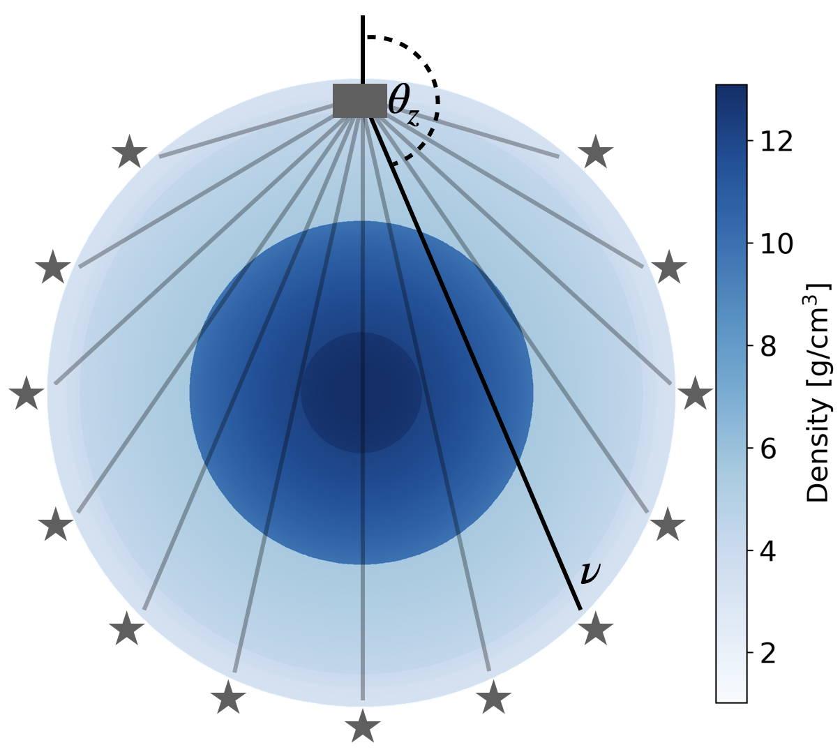
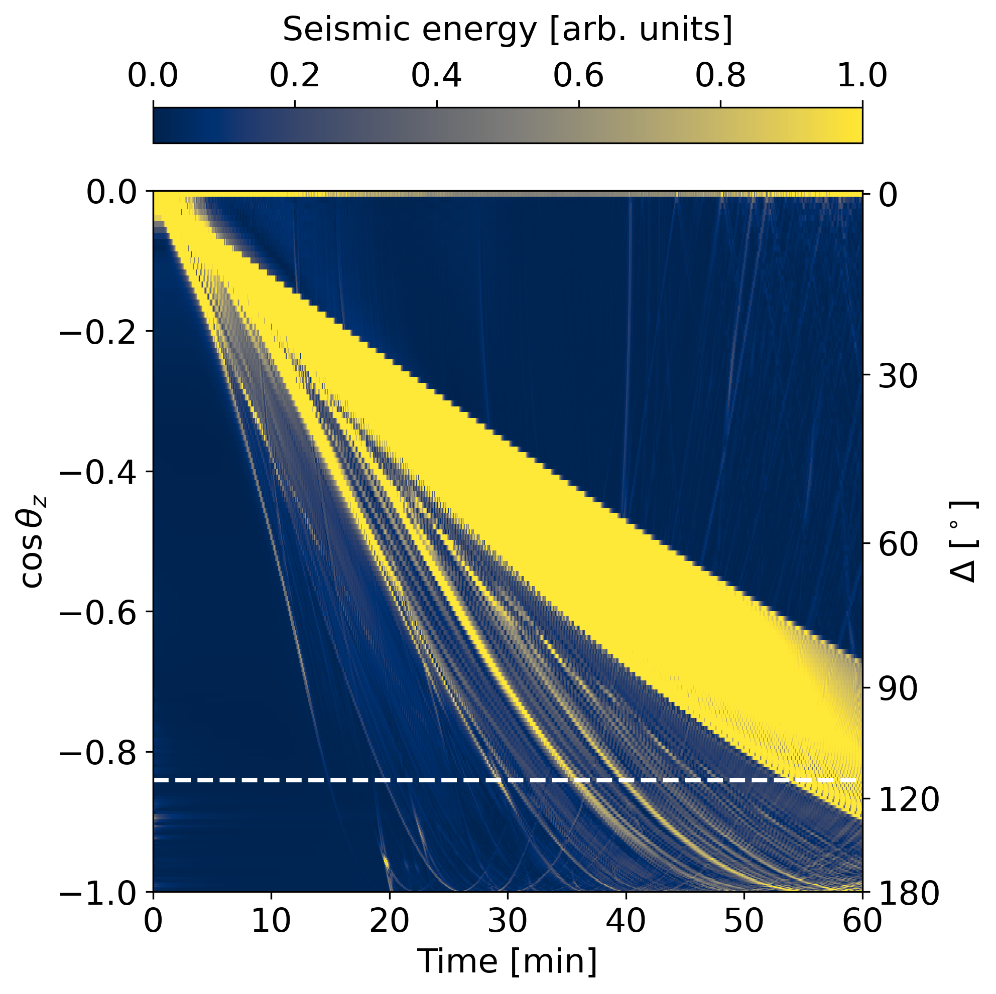
Neutrino oscillation tomography is based on the principle that neutrino oscillation probabilities are affected by the presence of matter (more precisely, electrons) along the neutrino path. The probability of a given oscillation process ν α → ν β is usually visualized in a 2D plot, referred to as oscillogram, as a function of neutrino energy E ν and incidence angle θ z . This angle is measured with respect to the vertical at the neutrino’s exit point on the Earth’s surface (see Figure 1a) and uniquely determines the neutrino baseline, which in turn defines the electron density profile encountered along the neutrino path through the Earth. As an example, figure 1c displays the oscillogram corresponding to the probability P matter νµ→ντ that a muon neutrino produced in the atmosphere is detected as a tau neutrino after having propagated across the Earth, assuming PREM, the Preliminary Reference Earth Model [14]. Values of cos θ z ≲ -0.84, or equivalently ∆ ≳ 114 • , where ∆ is the epicentral distance defined in Figure 1b, correspond to neutrinos traversing the core.

In Figure 1c, one can readily note how the density jump at the core-mantle boundary alters the neutrino oscillation pattern.

Neutrino oscillograms can be compared to what seismologists record, namely time-distance plots of seismic energy, obtained by considering a single earthquake and a network of seismic stations (see Figures 1b and1d). In NOTE, this situation is essentially reversed (see Figure 1a). Owing to their high cost and complexity, only a few neutrino detectors are built across the globe. Each of them will detect neutrinos produced in the atmosphere arriving from all directions. Consequently, in oscillograms the values of cos θ z (or ∆) scan over different neutrino sources, whereas in the seismic energy plot they correspond to different seismic stations.

For a fixed incidence angle, Figure 1c shows seismic energy as a function of time since the event. Neutrinos with a specific incidence angle take a fixed time t to propagate, measured in the laboratory frame. Since neutrinos travel almost at the speed of light c, according to special relativity the neutrino’s proper time t ′ , which is the time experienced in the reference frame of the moving neutrino, is proportional to t/E ν , where E ν is the neutrino energy. Thus, for a given incidence angle, proper time is inversely proportional to energy, and the x-axis of the oscillogram can be interpreted as a measure of the neutrino’s proper time, analogous to time in the seismic plot.

Another important difference between neutrino and seismic tomography arises from the fact that seismic waves are reflected and refracted by structures in the Earth’s interior, while neutrinos travel in straight lines (see Figure 1a). Once a neutrino’s incidence angle is measured, its trajectory and the region it probes are uniquely determined (within associated uncertainties), unlike seismic waves, which can traverse multiple regions for a given source-receiver pair (see the white station in Figure 1b). However, the large number of seismic stations in operation today, along with the accumulated set of earthquake observations, provides a dataset whose statistical power exceeds that of atmospheric neutrino events recorded so far. The advent of a new generation of neutrino detectors, as described in 4, is expected to significantly increase the neutrino dataset available for NOTE in the upcoming decades.

The oscillograms introduced in section 2 constitute only one component of the forward modeling chain used in NOTE. In order to estimate the sensitivity of the method to Earth’s interior properties, we need to simulate the expected rate of neutrino events at a given detector as a function of energy and arrival direction for a given Earth model. To that aim, we use the EarthProbe framework [51], which handles atmospheric neutrinos entering the Earth (see Section 3.1), computes their oscillation probabilities as they traverse the Earth’s interior (see Section 3.2), and models their detection (see Section 4). In Appendix A, we provide tables listing the physical constants and variables used in this study for easy reference.

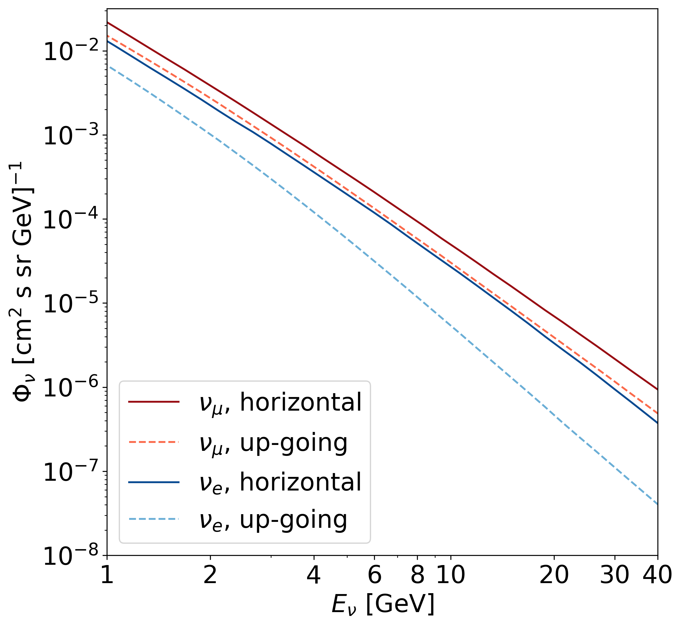
Neutrinos entering the Earth are modeled using the atmospheric neutrino flux of Honda et al. [52]. This model simulates the cosmic ray flux, its interactions, and the propagation, interactions, and decays of secondary particles in the atmosphere. It includes atmospheric density variations and [52], averaged over all azimuthal angles. Further details on the neutrino flux are provided in the text. Horizontal neutrinos (solid lines) correspond to cos θ z values between -0.1 and 0.0, while up-going neutrinos (dashed lines) span the range from -1.0 to -0.9. geomagnetic effects on charged particle trajectories, and provides differential neutrino fluxes as a function of energy and arrival direction at several reference experimental sites.

In this work, we use the benchmark flux computed for the Gran Sasso site (no mountain overburden), averaged over azimuth and seasonal variations, and assuming minimum solar activity [53]. Gran Sasso, which hosts the underground laboratory [54], lies at a latitude similar to that of the detectors considered here, and flux differences between these sites are expected to be within ∼ 1% [52]. Averaging over seasons is appropriate since NOTE will use data collected over several years. Solar activity effects are below 1% for neutrino energies above 3 GeV and reach at most 3% at lower energies [52].

Figure 2 illustrates how the neutrino flux decreases steeply with energy, reflecting the sharp decline of the cosmic ray flux that produces it (see, e.g., Chapter 30 of [35]). It emphasizes the importance of low-energy neutrinos for tomography studies since they provide significantly larger event statistics. Furthermore, this figure reflects that the atmospheric neutrino flux consists mostly of muon neutrinos, which are roughly twice as abundant as electron neutrinos, while tau neutrinos are rarely produced in air showers and appear only later through flavor oscillations.

Given that neutrinos interact only through the weak force and no muon and tau particles are present in the Earth, neutrino oscillation probabilities are mostly influenced by the electron density along their path through the Earth:

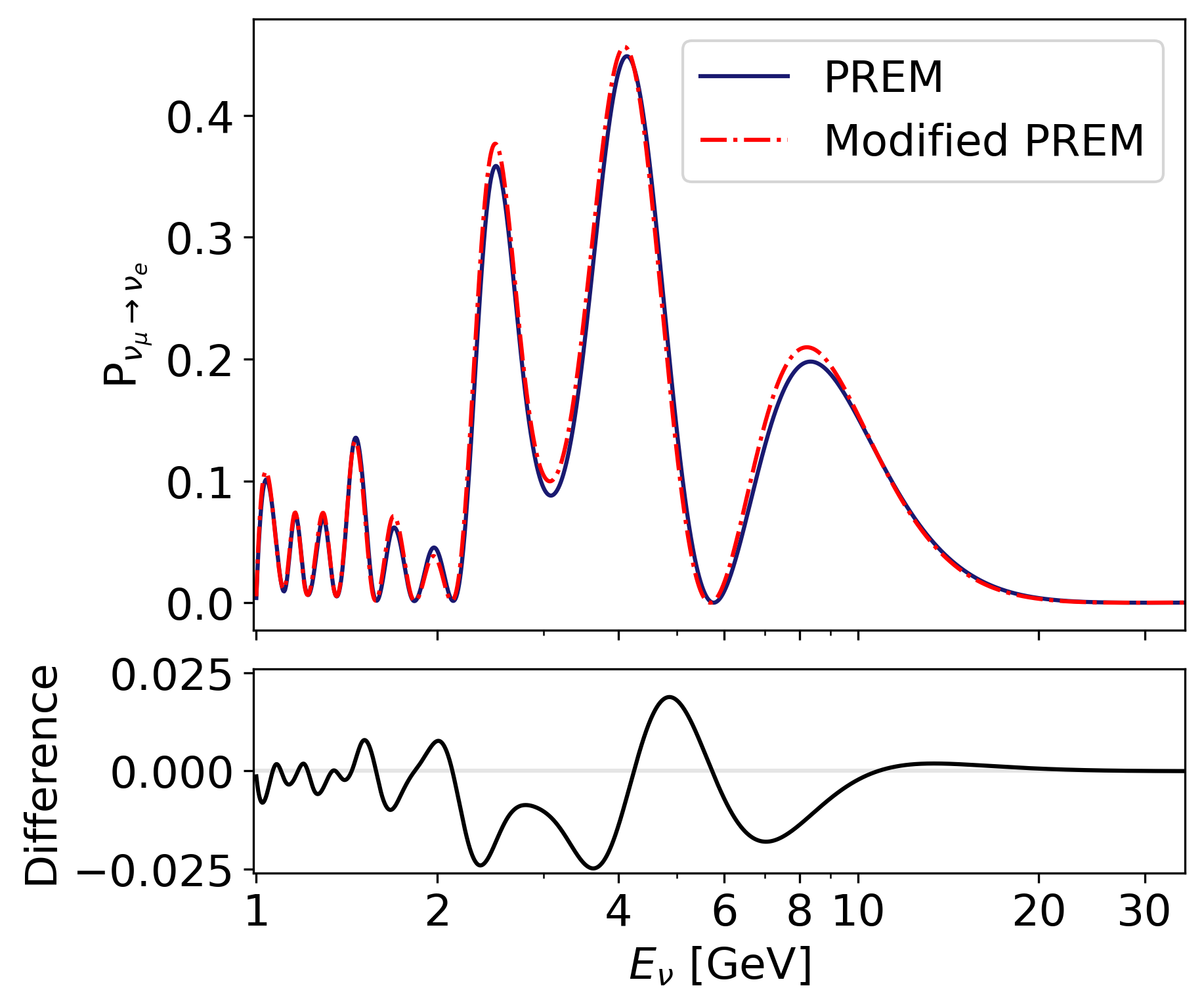
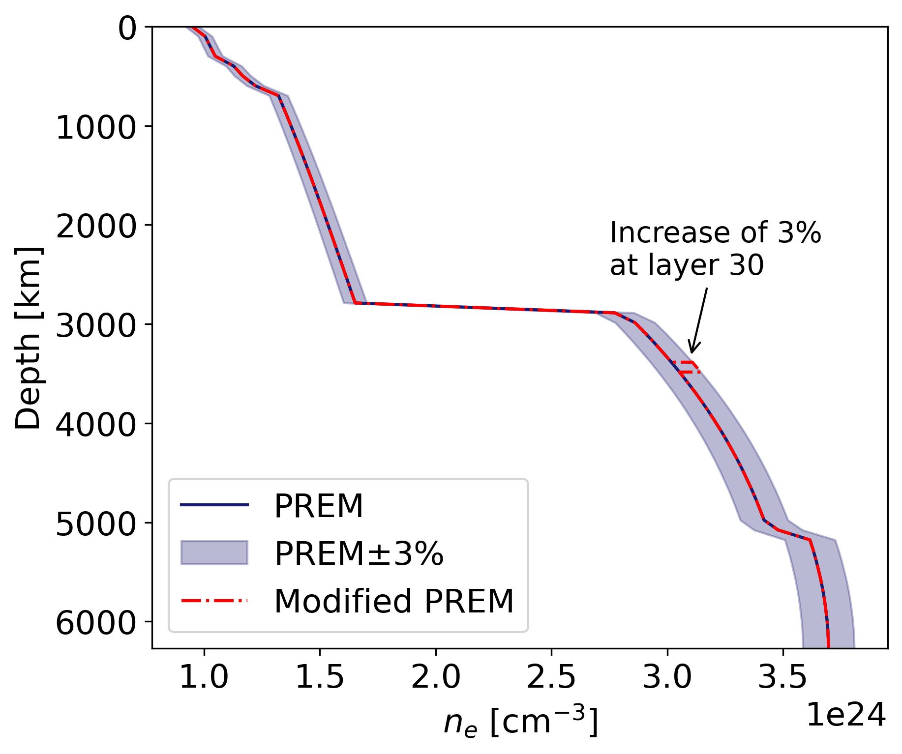
where ρ is the matter density, Y e is the electron yield, N A is the Avogadro number, and M u is the molar mass constant. The electron density defined in this way is expressed in number of electrons per cm 3 . EarthProbe can read user-defined ρ and Y e distributions. For our calculations, we adopt the PREM model [14] to define the Earth’s matter density profile as a function of depth. Unless stated otherwise, we discretize PREM into 64 equally thick layers of constant density ρ. We assign each layer an electron yield derived from GERM, the Geochemical Earth Reference Model [55],

following

where the sum is taken over all the elements present in that layer, w i is the weight fraction of the ith element, and Z and A are the atomic number and standard atomic weight, or proton-to-nucleon ratio, of the ith element, respectively. Y e reflects the chemical composition of a layer and has values close to 0.47 in the core and 0.5 in the mantle and crust. Figure 3a shows the resulting electron density as a function of depth.

The electron number density along a given baseline depends on the neutrino time-of-flight t (n e (t)). EarthProbe computes the evolution of the neutrino flavor state ν α (with α ∈ {e, µ, τ }) along this baseline by solving the Schrödinger equation with a time-dependent Hamiltonian:

where ℏ is the reduced Planck constant and H(t) is the effective Hamiltonian for the given baseline:

Here, the first term is the neutrino Hamiltonian in vacuum. Neutrinos are produced and detected in flavor eigenstates (electron, muon, tau), but they propagate as mass eigenstates. The transformation between these two bases is given by the Pontecorvo-Maki-Nakagawa-Sakata (PMNS) matrix U (the † denotes the Hermitian conjugate), which encodes the mixing angles Θ 12 , Θ 13 , Θ 23 and a complex phase δ CP , that govern neutrino oscillations:

Here

j are the differences of the squared neutrino masses.

The neutrino oscillation parameters (∆m 2 ij , Θ ij , δ CP ) used in EarthProbe are taken from the global fits performed by the NuFIT collaboration [56], which are regularly updated with new experimental data. Since the sign of ∆m 2 31 has not yet been established, the neutrino mass ordering, i.e. whether the masses are arranged as m 1 < m 2 ≪ m 3 (normal ordering) or as m 3 ≪ m 1 < m 2 (inverted ordering), remains unknown. The choice of mass ordering affects neutrino oscillation probabilities and therefore impacts this study. Throughout our analysis, we assume the normal mass ordering, which is currently slightly favored by global data [56].

The matter-induced potential is added with the second term in Equation (4):

where G F is the Fermi constant, n e (t) is the electron density profile, and the sign is positive (negative) for neutrino (antineutrino) interactions. For a comprehensive overview of this topic, we refer the reader to the review in [30].

To solve Equation (3) for a specific neutrino baseline, EarthProbe builds an array of the Earth matter segments successively traversed by the neutrino, each with constant electron density. The solution is then given by:

where T is the time the neutrino needs to cross the entire baseline and T is the time-ordering operator that ensures computations follow the correct temporal sequence of segment crossings. After discretizing the total time T into small intervals ∆t k , the OscProb package [57] is used to solve Equation ( 7) numerically, by approximating H(t) as a sequence of piecewise-constant Hamiltonians H(t k ), each defined over the time interval ∆t k :

Solving Equation ( 8) finally requires computing the matrix exponential of each 3 × 3 Hermitian matrix H(t k ). OscProb performs this operation efficiently by solving the eigensystem of each Hamiltonian using the hybrid algorithm described in [58], and computing the singular value decomposition of the symmetric matrix in the first term of Equation ( 4).

Once the evolution of the neutrino flavor states along a baseline is computed, the oscillation probability for the transition ν α → ν β (where {α, β} = {e, µ, τ }) is obtained by evaluating the squared inner product:

As an example, the transition probability P νµ→νe for PREM and for an alternative Earth model (illustrated with a red dash-dotted line in Figure 3a) are shown in Figure 3b.

In our sensitivity study in Section 5, we will compare expected neutrino rates computed using the reference Earth model with those obtained for alternative Earth models of interest. Figure 3b illustrates the subtle effect of the small density perturbation implemented in the alternative Earth model from Figure 3a on the oscillation probability P νµ→νe . Although the absolute difference is small, it contains the information needed to infer local heterogeneities, analogous to detrending tidal ground motions or measuring travel-time differences in seismology.

Once neutrinos reach the vicinity of the detector, they have a small probability of interacting and generating a detectable signature that can then be reconstructed. Section 4.1 describes how to compute the neutrino interaction rate in a target volume, independent of the subsequent detection technique. EarthProbe was originally designed to model water Cherenkov detectors, whose detection principle is outlined in Section 4.2, along with the approach used to emulate other detection media.

In the energy range of interest for NOTE, neutrinos interact primarily by scattering off nuclei in the medium [59]. Their interactions are classified according to whether a neutral (Z 0 ) or a charged (W ± ) weak-force boson is exchanged. The first case corresponds to neutral-current (NC) interactions, in which the neutrino remains in the final state and escapes the instrumented detector volume, while the scattered nucleus can produce a detectable signal. NC interactions are flavor-independent and can therefore be treated as a single type. The second case corresponds to charged-current (CC) interactions, where an incoming neutrino (antineutrino) ν α (with α ∈ {e, µ, τ }) produces a negatively (positively) charged lepton α -(α + ). In this case, both the scattered nucleus and the outgoing charged lepton can produce detectable signals. Neutrino interactions are thus separated into 8 channels, denoted by ν X : six for CC interactions, involving ν e , νe , ν µ , νµ , ν τ , ντ , and two for NC interactions, which involve ν, ν.

For each channel ν X , the differential rate of interactions with target nucleons is computed as a binned function of the energy and zenith angle, per unit exposure (defined as the product of running time and target mass of the detector) [49]:

To compute this rate, EarthProbe weighs the atmospheric neutrino flux by the corresponding probabilities to oscillate into the flavor associated to channel ν X or to stay in that flavor, and then multiplies the resulting flux at the detector by the channel-dependent cross section σ int ν X , which is a measure of the probability that the neutrino undergoes this interaction and is given in units of area (representing the effective target size):

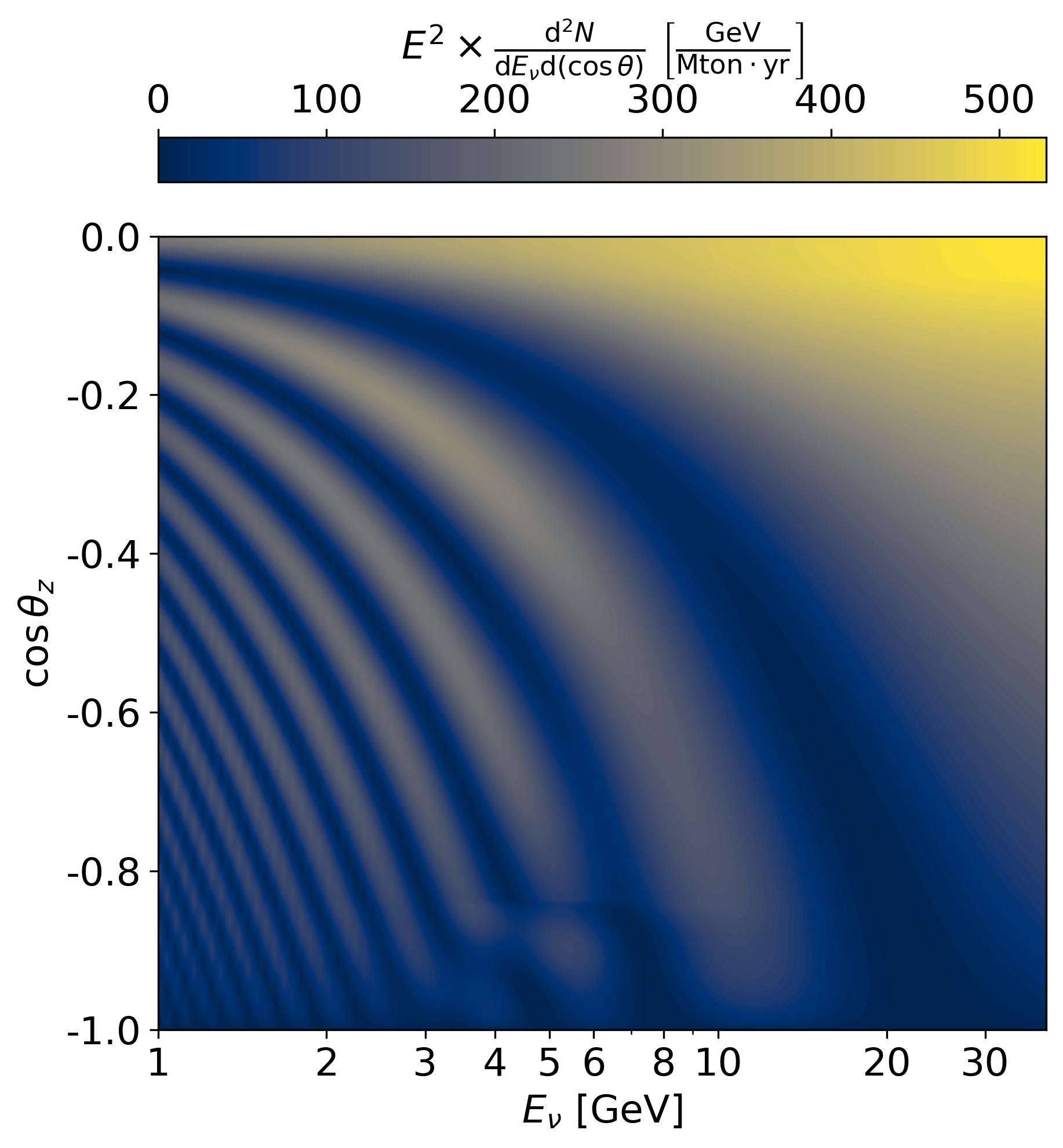
(11) Here, ν β ∈ {ν e , ν µ } (ν β ∈ {ν e , νµ }) when ν X is a neutrino (antineutrino) channel. Furthermore, the contribution of atmospheric tau (anti)neutrinos is neglected, as they are very rarely produced in extensive air showers. The cross section is divided by the average mass of the target nucleons in the medium, so that event rates for a given detector can be obtained by multiplying R int ν X by the detector mass. In this analysis, we consider 100 bins of logarithmic energy, from 1 GeV to 40 GeV, and 800 bins of cos θ z , from 0 to -1. These values were selected since the large exposure times explored in this study provide sufficiently high event statistics. Energies below 1 GeV are not considered, as the resulting sensitivity gain is negligible. E i ν and cos θ j z are the centers of the i-th energy bin and the j-th cos θ z bin, respectively. For a given detector exposure (the product of data-taking time ∆t and instrumented mass M ), the expected number of neutrinos interacting within the detector in a specific energy and incidence-angle bin, via channel ν X , are computed as:

As an example, Figure 4a presents the expected distribution of interacting neutrino events through the (ν µ + νµ ) CC channels, corresponding to a detector exposure of 1 Mton•years. At this step, the oscillatory behavior as a function of energy and incidence angle is still apparent (due to the multiplication by E 2 ν ). Investigating interacting neutrino event distributions for different Earth models reveals the channels, and (E ν , cos θ z ) regions where the intrinsic signal is strongest. In practice, observed distributions can deviate significantly due to the limited efficiency and resolution of real detectors in reconstructing neutrino energy, direction, and flavor.

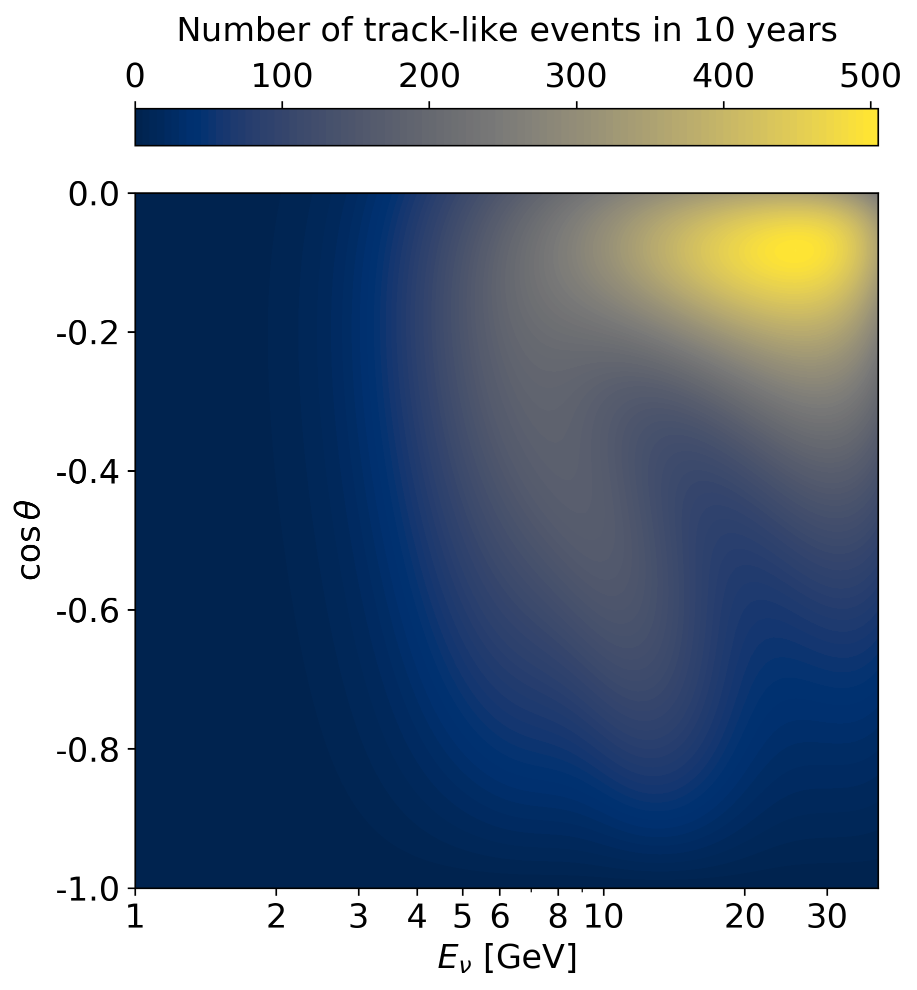
The reconstruction of neutrino properties in Earthprobe follows the logic of water Cherenkov detectors (WCD) such as KM3NeT/ORCA [60], a 3D array of photosensors currently being deployed deep in the Mediterranean Sea, which will cover around 6700 m 3 of water once completed. Such detectors identify neutrinos by capturing the Cherenkov light emitted when charged particles produced in neutrino interactions travel through the water faster than the phase velocity of light in that medium. The signatures that dominate the detectable signal arise from CC interactions of (anti)neutrinos. Electrons/positrons (the electron’s antiparticle) emerging from ν e /ν e interactions generate localized showers (similar to those generated by cosmic rays in the atmosphere, see Section 1), which give rise to roughly spherical distributions of Cherenkov light around the interaction point, and are referred to as shower-like events. Muons/anti-muons generated in ν µ /ν µ interactions, being much heavier and minimally scattering, produce track-like signatures, characterized by long patterns of Cherenkov photons (e.g. O(500m) for a muon of energy 100 GeV). The tau/anti-tau leptons produced in ν τ /ν τ interactions are even heavier, short-lived particles that can produce either type of event signature, depending on their decay channel. In approximately 17% of cases, the τ -/τ + decays into a µ -/µ + , producing a track-like event, while all other decay channels result in shower-like signatures. Scattered nuclei in both NC and CC interactions can also generate localized showers. Consequently, all neutrino interactions in a WCD such as KM3NeT/ORCA can be classified as either track-like or shower-like.

Reconstruction algorithms applied to data from WCDs exploit the spatial and temporal patterns of Cherenkov light detected by the optical sensors to estimate the type of signature generated by a neutrino event (track-like or shower-like), its arrival direction, and energy. However, the reconstruction accuracy is limited by detector factors, such as the number, density, and efficiency of photosensors.

To account for detector uncertainties and inefficiencies, EarthProbe uses a set of analytical functions modeling the detector response. These include smearing functions for the reconstruction uncertainties σ(E ν ) and σ(θ z ) in energy and zenith angle, and efficiency functions ϵ det (E ν ) and ϵ class (E ν ), which respectively represent the probability of successfully detecting a neutrino interaction, and the probability of correctly classifying an interacting event into the corresponding topology (e.g., classifying a ν µ CC interaction as tracklike). The efficiency ϵ det (E ν ) is zero below the detector’s energy threshold. All functions are parametrized with a small number of user-defined parameters (for full details, see [49]). This approach is sufficiently flexible to emulate detector technologies other than WCDs. Benchmark parametrizations are provided for KM3NeT/ORCA, the WCD Hyper-Kamiokande [61] (HK), and DUNE [62], which uses liquid argon as its detection medium. All results in Section 5 use these ORCA-like, HK-like, and DUNE-like parametrizations from [49]. The idealized next-generation detector used in the present work is defined in Section 5 and differs from the one used in [49].

In this section, we analyze the sensitivity of NOTE to a 3% increase in the electron density n e of any ∼100 km-thick layer. Specifically, for each layer, we compare, for a given detector, the expected neutrino event rates obtained using the PREM model with those obtained after increasing n e by 3% relative to PREM in the layer. To isolate the net impact of the n e increase in a single layer, we disregard, at this stage, the small perturbations induced by this modification on the Earth’s total mass and moment of inertia. We simulate the expected neutrino events over a benchmark 20-year data-taking period, typical of current detectors.

To estimate the intrinsic sensitivity of the method, we compute the expected event rates for a hypothetical next-generation detector with nearperfect reconstruction capability. We consider minimal systematic uncertainties on the reconstructed neutrino energy and incidence angle arising from the stochasticity in the kinematics of interactions due to nuclear Fermi motion. The energy resolution is negligible, while the angular resolution appropriate for this scenario is:

We assume that such a detector has the capability to perfectly identify all eight interaction channels described in Section 4.1 and is fully efficient in detecting neutrino interactions over the energy range of interest, i.e., ϵ eff (E ν ) = 1 for E ν ≥ 1 GeV.

Since the previously described detector requires technological advances beyond current funding limits, we also consider a more realistic configuration based on state-of-the-art WCDs, but pushed to its performance limits. We use the same detection efficiency, angular, and energy resolutions as above, but assume it can perfectly distinguish only track-like from showerlike events. This corresponds to a classification efficiency ϵ class (E ν ) = 1 at all neutrino energies. For both detectors, we adopt a benchmark instrumented mass of 10 Mton, yielding a total exposure of 200 Mton•years.

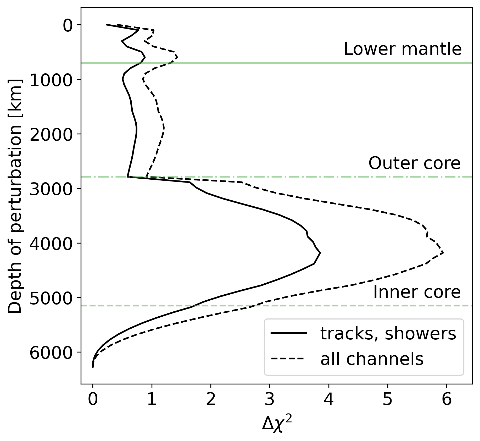
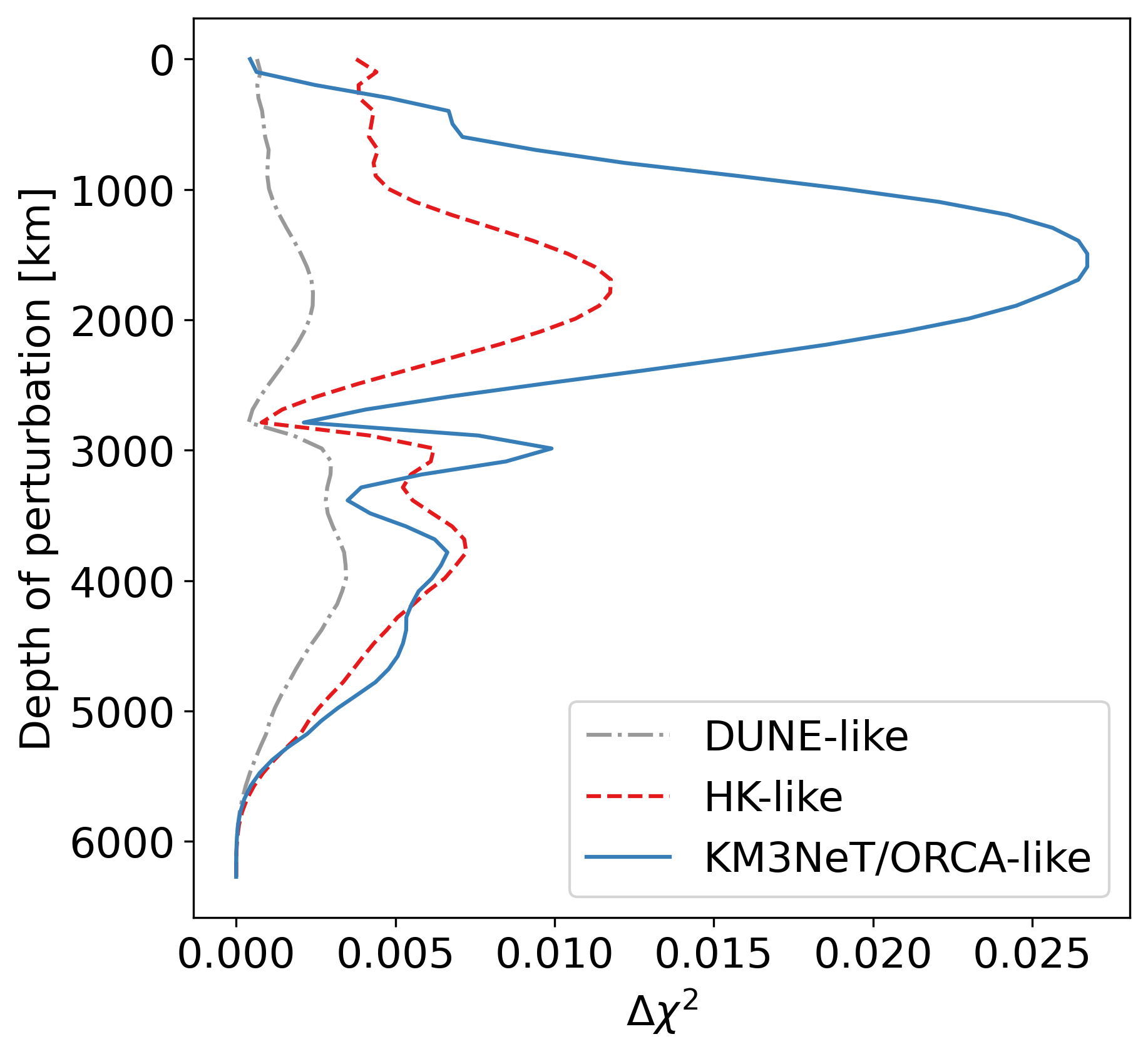
As a measure of the sensitivity for these hypothetical next-generation detectors to distinguish between two electron density scenarios, we report in Figure 5a the total ∆χ 2 values, computed as where the summation goes over all N E energy bins and N θ incidence angle bins (see [49] for further details on the mathematical formalism). N PREM i,j and N mod i,j denote the numbers of registered neutrino events for the reference and modified Earth models, respectively. The binning described in Section 4.1 is sufficiently fine to approximate the limit of infinitely small bins. The values shown in Figure 5a should be interpreted as the statistical significance with which PREM would be rejected if the event counts N mod i,j in Equation ( 14) were observed.

The intrinsic sensitivity of NOTE to increases in electron density is found to be highest for the Earth’s outer core, for either type of hypothetical nextgeneration detector. It decreases sharply toward the Earth’s center, as fewer neutrinos are available to probe layers with decreasing size. Moreover, near the Earth’s center, the longest neutrino path through a layer is shorter, further limiting its impact on oscillations. The sensitivity to changes in the mantle density is significantly lower and declines toward the Earth’s surface. This trend is largely due to the fact that lower-density layers correspond to higher resonance energies (see Section 1), where the atmospheric neutrino flux is lower, leading to reduced event statistics and consequently decreased sensitivity.

Figure 5b presents sensitivity curves computed analogously to Figure 5a, but now including detector effects corresponding to the DUNE-, HK-, and KM3NeT/ORCA-like configurations. Many of the qualitative features observed previously are preserved, though the overall sensitivity is significantly reduced, owing to the limited event reconstruction and identification capabilities of these detectors.

The decrease in sensitivity is more pronounced in the core region because neutrinos traversing the core experience resonant matter effects at energies close to 3 GeV, as opposed to ∼7 GeV for neutrinos crossing only the mantle. Since the performance of event reconstruction and identification worsen at lower energies for all considered detectors, 3 GeV neutrinos are reconstructed less accurately than 7 GeV neutrinos. Consequently, the sensitivity to density modifications degrades more rapidly for the core than for the mantle, with the effect being strongest for KM3NeT/ORCA, intermediate for Hyper-Kamiokande, and smallest for DUNE, reflecting the corresponding resolutions and efficiencies. In the case of the ORCA-like detector, the pronounced loss of sensitivity for the core arises not only from its poorer energy and angular resolutions, but also from its higher energy threshold. The detection efficiency reaches its maximum around 5 GeV (see Figure 4 in [49]).

In conclusion, our results suggest that achieving the best sensitivities to both the Earth’s core and mantle requires detectors with a detection threshold well below 3 GeV (achieved in the DUNE-like and HK-like detectors), good energy and angular resolution at low energies (as in the DUNE-like detector) as well as sufficiently large detector volumes (as in the KM3NeT/ORCA-like detector). While the technology to build such a detector may become available on a reasonable timescale (for example, a more densely instrumented version of KM3NeT/ORCA could provide these favorable conditions) the main limitation remains the associated cost.

In this section, we focus on two regions of the Earth that are of particular geophysical interest and analyze the sensitivity of NOTE to their electron density variations relative to PREM. To obtain realistic sensitivity projections, we account for the global constraints imposed by the Earth’s total mass and moment of inertia (as suggested in a recent work [50]).

Seismic imaging has repeatedly revealed low-velocity and low-attenuation regions within and just below the Mantle Transition Zone (MTZ) [63,26,27]. These anomalies may be due to the presence of water, since laboratory experiments show that the main minerals in the MTZ, wadsleyite and ringwoodite, can incorporate significant amounts of water into their crystal structures as hydroxyl (OH -) groups [see e.g. 21]. Incorporation of water affects their anelastic modulus, but the sensitivity of seismic attenuation to water content remains poorly constrained [20], and seismic attenuation itself is difficult to image. Complementary measurements are therefore needed to conclusively link these low velocities to the presence of water [64]. If the MTZ contains more water locally than previously assumed [63,19,20], its electron density would deviate from PREM and could therefore be detectable through NOTE. Hydrogen increases Y e (which affects the electron density, see Equation ( 1)), as it has the highest proton-to-nucleon ratio, (Z/A) H ≈ 1 (the protium lacks a neutron). At the same time, adding hydrogen to major mantle minerals also changes their molar mass and unit-cell volume [22,23], thereby influencing mass density (possibly lowering it). The net effect is thus a trade-off between these contributions. Consequently, we examine how the sensitivity to MTZ properties varies under modifications of the electron density of up to ±1%, while the interpretation of these changes is beyond the scope of this paper.

Since the MTZ is approximately 250 km thick (extending from a depth of ∼410 km to ∼660 km), we discretize the Earth’s electron density profile into 128 depth bins of equal thickness for this study. To satisfy the two global constraints mentioned above, for each percent modification of the MTZ electron density, we rescale independently the n e distribution in the unchanged core and the n e distribution in the modified mantle. As a result, the percentage initially applied to the MTZ electron density is multiplied by the correction factor required for the mantle. The value of ∆n e /n e in Figure 6 is the actual percent modification relative to PREM.

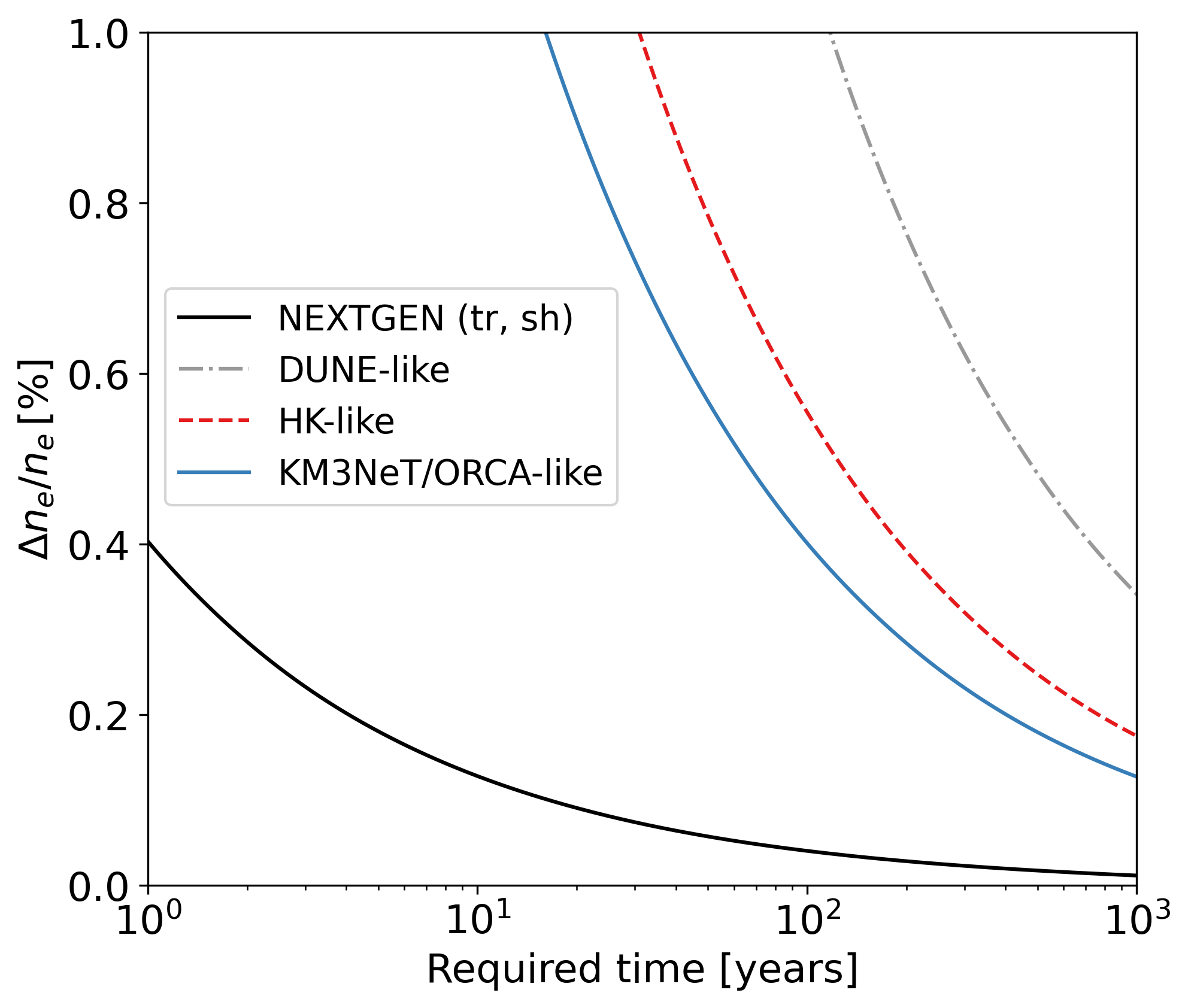
Figure 6a shows the required data-taking time to achieve a 1σ rejection of PREM for a given change in electron density. We present a best-case scenario (full black line) using the hypothetical next-generation detector capable of accurately distinguishing track-and shower-like events (see Sections 4.2 and 5.1), and the projections for the DUNE-, HK-, and KM3NeT/ORCAlike configurations. Since the considered perturbations are small, an increase or decrease of a given percentage in electron density yields approximately the same sensitivity. Consequently, the results can be expressed in terms of ∆n e /n e . Among the state-of-the-art detectors, KM3NeT/ORCA offers the most favorable time projection, owing to its large size, although the required data-taking time exceeds 1000 years for all considered electron density modifications. Within 100 years of data-taking time, a KM3NeT/ORCA-like (HK-like) detector would be able to measure a n e change in the MTZ of about 3.4% (4.8%). The next-generation scenario suggests that substantial improvements could be realized with upgraded detector capabilities, while the required data-taking time is inversely proportional to the detector size.

Seismological observations suggest that the matter density of the core may be between 0.94% and 1.25% higher than in PREM [15]. In [65], the authors show that the light-element content in the Earth’s inner core may be up to twice as large as previously estimated. Additionally, if hydrogen is introduced into the outer core, as suggested by mineralogical studies [e.g. 24,25], it could modify its matter density by up to 1%. The electron density n e may vary differently, due to associated changes in the electron yield Y e .

We therefore study how the sensitivity of NOTE depends on the magnitude of the electron density modification in the entire core, by up to ±1%.

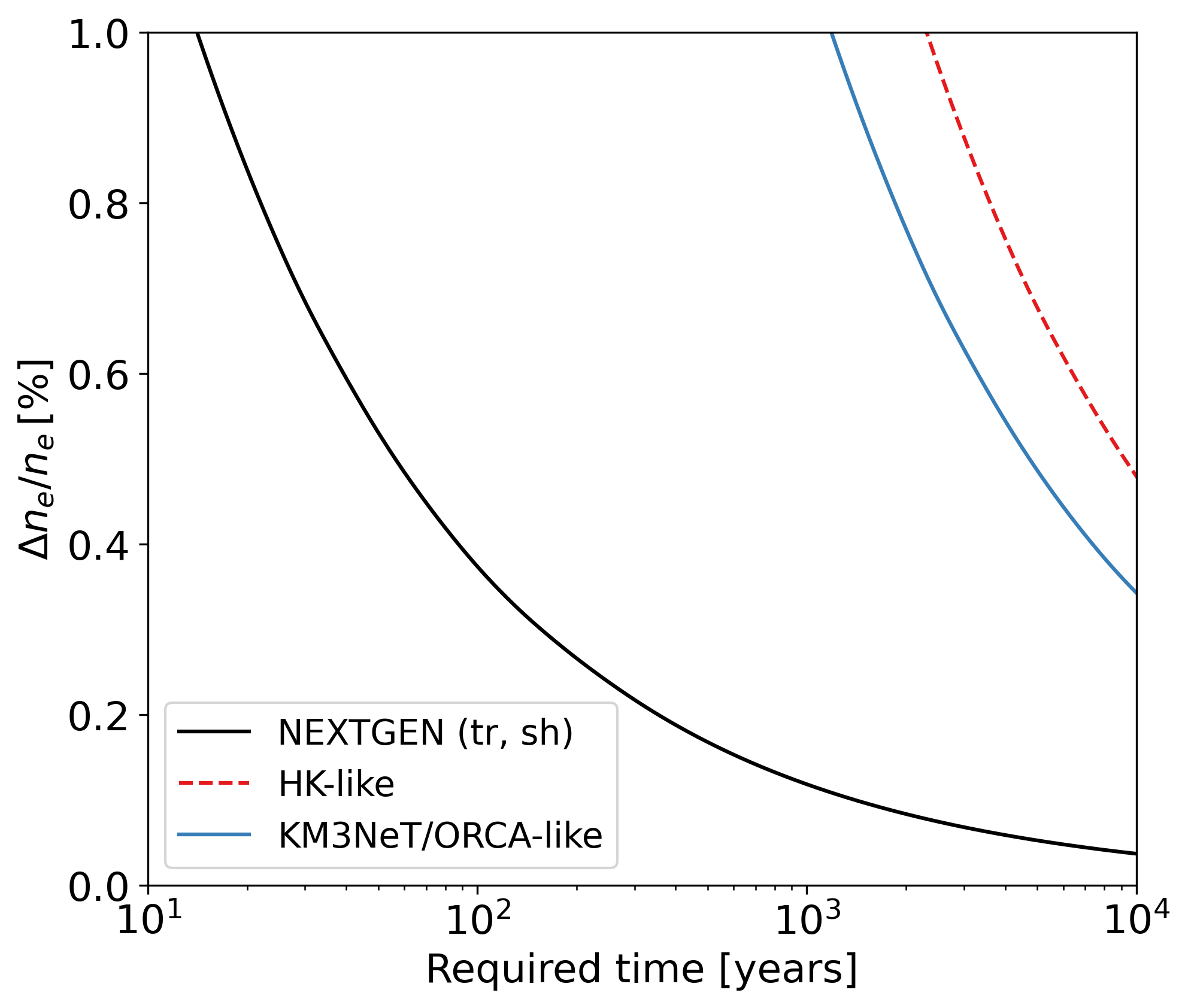
Since we modify the electron density of the core, we rescale independently the lower mantle n e and the overlying mantle n e to satisfy the two global constraints. The corresponding data-taking time projections for the same detector configurations as in Figure 6a are shown in Figure 6b. Due to the high density and large volume of the core, the required exposure time for each detector is more favorable than for the MTZ analysis. For a density change of ∆n e /n e = 1%, the required data-taking time is close to 16 years (31 years, 117 years) for a KM3NeT/ORCA-like (HK-like, DUNE-like) detector. Within 10 years of data-taking, a KM3NeT/ORCA-like (HK-like, DUNE-like) detector could measure a density change in the core of approximately 1.3% (1.8%, 3.5%). These sensitivity projections outperform those obtained in [49] for the three current detectors, primarily due to the stronger density contrast introduced when adapting the n e profiles to satisfy the global constraints. The same effect enhances the performance of the next-generation detector considered here, though in that case the improved detector sensitivities also contribute to the gain relative to the “NextGen” benchmark in [49].

Research on the Earth’s internal structure has advanced greatly over the past century. Yet, several key questions remain open, such as the precise density and hydrogen content of different layers, motivating the search for new, independent observables that complement traditional geophysical methods. One promising observable is the flux of atmospheric neutrinos traveling through the Earth’s interior. In this contribution, we highlight ongoing interdisciplinary efforts to integrate neutrino oscillation measurements into studies of the Earth’s deep structure.

Using the EarthProbe software, we analyzed the sensitivity of neutrino oscillations to a 3% increase in electron density within nearly 100 km-thick layers, as a function of the layer’s depth. We considered two idealized detectors that approach the fundamental limit set by the stochastic nature of neutrino interactions. The first detector, capable of distinguishing all interaction channels, represents the ultimate theoretical limit of sensitivity, while the second detector, distinguishing only track-and shower-like topologies, represents a more realistic yet still highly performing configuration. We then extended the study to the three state-of-the-art detectors KM3NeT/ORCA, Hyper-Kamiokande, and DUNE. Furthermore, we examined how the datataking time required by these detectors to measure a 1σ modification of the electron density in the MTZ and the core with respect to the PREM model depends on the magnitude of the density perturbation.

Our results indicate that observing a 1% modification of the core electron density relative to the reference model at the 1σ level would require 16 years (31 years) of exposure in a KM3NeT/ORCA-like (HK-like) detector. A corresponding modification of the MTZ would require more than 1000 years of observation. Measuring smaller deviations would demand longer datataking times, which for the study of the core could potentially be feasible by combining data from multiple neutrino observatories. KM3NeT/ORCA is steadily accumulating data [66], while Hyper-Kamiokande and DUNE are scheduled to begin data-taking in the coming years, enabling the combination of neutrino observations from multiple detectors to probe the Earth’s interior.

In our analysis, the hypothetical next-generation detectors outperform the configurations currently under construction, hinting at potential directions of improvement in future experiments. The performance of a neutrino detector is governed by its energy and angular resolutions, its ability to distinguish neutrino flavors and interaction mechanisms, and its effective target volume. Future work should explore which specific detector characteristics most effectively enhance sensitivity to different Earth regions, guiding the design of the next generation of instruments. In particular, it would be valuable to identify the detector requirements for probing the MTZ.

Finally, the methodology for computing neutrino rates outlined in this paper also allows us to compute sensitivity kernels, which opens an avenue to perform joint inversion of neutrino and seismic data in the near future. Although differences in resolving power exist for various regions and parameters, such a combined approach could provide an improved view of the Earth’s interior.

the Institut Universitaire de France. Eric Mittelstaedt and Yael Deniz were supported by the Award 2406115 from the United States National Science Foundation.

In this appendix, we provide tables listing the physical constants and variables used in this study.

📄 Read Full PDF on ArXiv

This content is AI-processed based on open access ArXiv data.