KANFormer for Predicting Fill Probabilities via Survival Analysis in Limit Order Books

Electronic financial exchanges commonly use limit order books (LOBs) to match buy and sell orders across various asset classes. Among the order types supported by LOBs, limit orders, market orders and cancel orders are the most frequently used [Abergel et al., 2016, Gould et al., 2013]. Unlike market orders, which execute immediately at the prevailing bid or ask, limit orders are placed at predefined prices to seek a more favorable execution. Although limit orders can yield more favorable prices, they carry the risk of non-execution: these orders remain in the book until they are either matched with an incoming market order or canceled before execution. Therefore, it is crucial for investors to assess the likelihood that a limit order will be executed within a given time horizon. The time a limit order remains in the book before execution, referred to as its time-tofill, can vary widely and depends on the dynamics of the LOB [Arroyo et al., 2024, Maglaras et al., 2022]. Predicting the time-to-fill distribution or, equivalently, fill probabilities of limit orders plays a critical role in optimal execution strategies and has attracted significant research attention [Cho and Nelling, 2000, Lo et al., 2002a, Maglaras et al., 2022, Arroyo et al., 2024].

The time-to-fill of a limit order is inherently subject to right-censoring [Lagakos, 1979]: many orders are canceled or expire (i.e., remain in the LOB until the end of the trading day) without being executed, leaving their true fill times unobserved. This makes survival analysis, a statistical framework for censored time-to-event data, a natural tool for modeling and predicting the time-to-fill of limit orders [Lo et al., 2002a, Maglaras et al., 2022, Arroyo et al., 2024].

Survival analysis has a long tradition in statistics [Cox, 1972] and, more recently, has been combined with deep learning to handle high-dimensional data and improve predictive power [Kvamme et al., 2019, Rindt et al., 2022, Bleistein et al., 2024]. Its application to limit order books began with econometric models of execution risk based on survival functions [Lo et al., 2002a], and was later extended to capture execution dynamics under censoring [Maglaras et al., 2022, Arroyo et al., 2024]. Building on this line of work, deep learning approaches specifically tailored to LOB data have emerged, including recurrent neural networks (RNNs) [Maglaras et al., 2022] and Transformer architectures [Arroyo et al., 2024]. However, these methods still face limitations in input representation, evaluation protocols, and interpretability, which we revisit in Section 2.

In this paper, we propose a new deep-learning-based survival analysis model, KANFormer, to model the fill probabilities of limit orders. Our key contributions are as follows:

-Rich input features beyond LOB snapshots: Prior models rely exclusively on LOB state features such as prices and volumes at different levels [Arroyo et al., 2024, Maglaras et al., 2022]. We extend this representation by incorporating agent-level behavioral data, namely order submissions, cancellations, and modifications, which provide additional insights into market dynamics that are not observable from LOB snapshots alone. -Comprehensive evaluation metrics: To rigorously evaluate model performance, we employ both calibration and discrimination metrics, addressing shortcomings in prior work that relied on incomplete metrics [Maglaras et al., 2022, Arroyo et al., 2024]. Specifically, we assess calibration using the Right-Censored Log-Likelihood (RCLL) [Balakrishnan and Mitra, 2012] and the time-dependent Brier score [Gerds and Schumacher, 2006], and discrimination using the C-index [Uno et al., 2011] and time-dependent AUC [Lambert and Chevret, 2016]. This dual approach ensures that the predicted survival distributions are both well-calibrated and properly ranked. -KAN-enhanced Transformer architecture: We propose a dual-encoder Transformer in which the standard feed-forward networks (FFNs) are replaced by Kolmogorov-Arnold Networks (KANs) [Liu et al., 2024]. Inspired by recent applications of KANs to time series forecasting [Genet and Inzir-illo, 2024a,b, Han et al., 2024, Zhang et al., 2024], this design strengthens nonlinear approximation while preserving the attention backbone [Vaswani et al., 2017]. -Model interpretability: We employ SHAP (SHapley Additive exPlanations) [Lundberg and Lee, 2017] to visualize global feature importance and track how different input features influence fill probabilities over time. This provides insight into the mechanisms driving execution risk and highlights the roles of both market and agent-level signals.

The remainder of this paper is organized as follows. Section 2 reviews related literature and discusses the limitations of prior approaches. Section 3 formulates the prediction task as a survival analysis problem. Section 4 introduces the KANFormer architecture. Section 5 presents empirical results, including benchmark comparisons, ablation studies, and feature attribution analysis. Finally, Section 6 concludes with future research directions.

This section provides the necessary background on limit order books (LOBs), survival analysis, and their application to modeling order execution. We begin with the operational structure of LOBs, then introduce the survival analysis framework and its relevance for execution modeling. We next review prior work and highlight their main limitations, which directly motivate our proposed approach.

LOBs are the primary mechanism by which modern exchanges facilitate trading across asset classes. A LOB displays all incoming orders with their price and quantity, matching buy and sell orders based on price-time priority. The bid side contains buy limit orders sorted by descending price, while the ask side contains sell orders sorted by ascending price. The best bid and ask define the top of the book, and their difference is the bid-ask spread [Bouchaud et al., 2009].

Order matching typically follows a price-time priority rule: better-priced orders execute first, and among equal prices, earlier orders take precedence. Unexecuted limit orders enter a queue and wait to be matched or canceled. The time-to-fill of a limit order therefore depends on queue position, incoming order flow, and broader market activity [Cartea et al., 2015]. A line of queuereactive models emphasizes this mechanism explicitly: Huang et al. [2015], Wu et al. [2019] simulate order-level behavior by tracking positions in the queue, while Cartea et al. [2014] highlight the importance of queue priority for optimal execution strategies. These studies underline queue position as a key determinant of fill probabilities, a feature we explicitly incorporate in our framework.

Because many orders are canceled or expire without execution, right-censoring is pervasive. This naturally motivates the use of survival analysis as a principled tool for modeling time-to-fill [Arroyo et al., 2024, Maglaras et al., 2022].

A common line of work casts LOB prediction as a classification problem at a fixed horizon H (e.g., mid-price up/down/unchanged [Zhang et al., 2019]). While intuitive, this framing has important drawbacks for execution modeling: (i) it imposes an arbitrary horizon H, (ii) censored orders (canceled or still active at H) are discarded or misclassified, and (iii) it ignores the timing of execution beyond H.

In contrast, survival analysis, a framework explicitly designed for time-toevent data under censoring [Kalbfleisch and Prentice, 2002], directly models the time-to-fill distribution under censoring, providing both horizon-specific discrimination (e.g., time-dependent AUC [Kamarudin et al., 2017]) and calibration of the full predictive distribution (e.g., Negative Right-Censored Log-likeLihood (RCLL)). Formally, let us denote T ∈ R + the duration between the upcoming execution time and the current time, with covariates x ∈ R p . Since T is not always be observed, we introduce a censoring time C ∈ R + , which corresponds to cancellation or expiration at market close. The observed time is then

where δ = 1 if the order is executed (partially or fully) and δ = 0 if it is censored (the order is canceled or expires before execution). A dataset of n orders is thus represented as

It is central to predict the survival function:

which gives the probability that an order remains unexecuted beyond duration t, with t being the duration measured relatively to the current time.

In survival analysis, it is standard to assume that, conditional on covariates x, the censoring time C and the event time T are independent [Leung et al., 1997]. This assumption, known as independent censoring, ensures that censored observations do not bias inference on execution times. Under this assumption, parameters can be optimized by minimizing the RCLL [Kalbfleisch and Prentice, 2002]:

which properly accounts for both executed (δ i = 1) and censored (δ i = 0) orders [Arroyo et al., 2024].

The time-to-fill of a limit order has long been studied under survival frameworks. Handa and Schwartz [1996] first modeled how traders balance price improvement against execution risk, and Lo et al. [2002b] later applied survival analysis to LOB snapshots. More recently, deep learning models have been proposed to predict survival curves directly from LOB snapshots [Arroyo et al., 2024, Maglaras et al., 2022]. For instance, Arroyo et al. [2024] introduced a convolutional-Transformer encoder combined with a monotonic neural network decoder [Rindt et al., 2022]. Different approaches have been adopted for evaluation. Arroyo et al. [2024] utilized the RCLL [Kalbfleisch and Prentice, 2002], which evaluates the overall quality of the predicted survival distribution. In contrast, Maglaras et al. [2022] focused on discrimination metrics such as the time-dependent AUC [Hung and Chiang, 2010], which measures the ability to distinguish between executed and unexecuted orders at a specific time horizon. Other metrics commonly employed include the Brier score [Graf et al., 1999], a horizon-specific measure of squared error, and the C-index [Harrell Jr et al., 1996], a global measure of concordance for order ranking. Former works typically adopt only a subset of these metrics: for example, some focus exclusively on time-dependent AUC or C-index, while others rely solely on RCLL.

Beyond evaluation metrics, recent advances have also focused on enhancing predictive performance through more sophisticated model design. Kolmogorov-Arnold Networks (KANs) [Liu et al., 2024], originally introduced as spline-based universal function approximators, have shown strong performance in sequential prediction tasks [Genet and Inzirillo, 2024a,b, Han et al., 2024, Zhang et al., 2024]. Replacing the feedforward layers of Transformers with KAN blocks yields KAN-Transformers, which offer enhanced expressive capacity and generalization. To our knowledge, these architectures have not yet been applied to survival analysis or execution modeling.

As far as interpretability is concerned, prior work has mainly relied on global feature importance techniques. In particular, Arroyo et al. [2024] applied SHAP values to identify which LOB features contribute most to the predicted execution risk. Their analysis focuses on feature importance computed at observed event times, providing a static view of explanatory factors within the survival modeling framework.

The discussions above highlight important foundations but also reveal limitations:

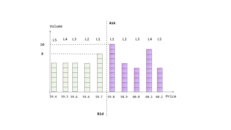
-Restricted representation of input: Most existing models rely on LOB snapshots (e.g., price and volume levels) as input data, while neglecting agent-level actions. Figure 1 illustrates two consecutive LOB snapshots in which the volume at the best bid decreases from 8 to 7 between t and t + 1. 1. Comparison of survival model evaluation metrics. RCLL evaluates calibration of the full predictive distribution, whereas Brier score and time-dependent AUC assess performance at specific horizons. The C-index is a global ranking measure. Practical readability refers to how easily the absolute value of a metric can be interpreted. For example, AUC and C-index correspond to probabilities of correct ranking, whereas the RCLL depends on data scale and therefore lacks a direct intuitive meaning in absolute terms. This change may arise from two distinct causes: (i) a market order consuming one unit at the best bid, or (ii) the cancellation of a standing bid order. Although the observed LOB update is identical, the underlying mechanisms, and their informational content, differ fundamentally. -Incomplete and hard-to-interpret evaluation protocols: Time-dependent AUC, time-dependent Brier score, and C-index, although informative, may not capture the full quality of survival predictions [Rindt et al., 2022]. Relying solely on discrimination metrics such as the AUC or C-index can obscure calibration performance, i.e., whether predicted survival probabilities align with observed outcomes. Conversely, while some works emphasize the RCLL for its statistical rigor in evaluating the overall quality of the predicted distribution, its practical readability is low, making it difficult to interpret and compare in practice.

We use the term practical readability to denote how easily a metric’s numerical value can be understood and compared in practice. For example, the Brier score corresponds to a mean squared error at a given horizon, and both the C-index and AUC can be interpreted as proba-bilities of correct ranking: concepts that are intuitive to practitioners. By contrast, the negative right-censored log-likelihood (RCLL) evaluates the fit of the entire predicted survival distribution. Although RCLL is a statistically principled [Rindt et al., 2022], its absolute values depend on data scale and context, making them less directly comparable and harder to interpret in practice. Table 1 summarizes the main properties of these metrics. Such incomplete evaluation protocols may lead to misleading conclusions. To address this, we adopt a comprehensive evaluation strategy that considers both calibration and discrimination. We provide further discussion on this issue, as well as the definitions of these metrics, in Appendix B.

-Limited model expressiveness: Transformer-based architectures have been used, but their reliance on standard feedforward layers overlooks newer approaches to modeling nonlinearity. More powerful alternatives, such as Kolmogorov-Arnold Networks (KANs) [Liu et al., 2024], which offer enhanced expressive capacity and generalization [Genet and Inzirillo, 2024a,b, Han et al., 2024, Zhang et al., 2024], remain unexplored in this context. -Static interpretability: Although prior work, such as Arroyo et al. [2024],

applied SHAP to obtain global feature importance, their analysis was restricted to observed event times. This provides only a static snapshot of explanations and does not capture how the contribution of features evolves across prediction horizons, which is essential for dynamic trading strategies.

These limitations motivate the need for a model that combines richer input features, more expressive architectures, comprehensive evaluation metrics, and dynamic interpretability. In Section 4, we address these challenges by integrating agent-level information, introducing KANFormer that provides both accurate predictions and interpretable insights.

In this section, we formulate the estimation of fill probabilities as a survival analysis problem, following the framework introduced in Section 2.2. For each studied order at the best ask/bid level, the objective is to predict its survival curve, which gives the probability that the order remains unexecuted beyond any time horizon. Execution is defined as the order being at least partially filled, while censoring occurs if the order is canceled or expires before execution.

As introduced in Section 2.2, survival analysis provides a principled framework for modeling time-to-event data under censoring. In our setting, the event of interest is the first execution of a limit order, which may be partial or full. To formalize, for an order i placed on the current, we denote (all times are expressed in seconds relative to midnight of the current day ):

t S i : the submission time of the studied order i t 0 i : the current time from which survival curve is modeled, δ i : label for execution (δ i = 1 if the order is executed on the current, otherwise δ i = 0) t * i : time of cancellation (resp. execution) if the order is canceled (resp. executed) t e : time when market closes on the current -T C i : duration defined as

Formally, given the market signals X just before t 0 i , the goal is to learn a model that outputs the survival function for all t > t 0 i .

This formulation follows directly from the general setup in Section 2.2, but specializes it to the microstructural context of LOBs.

Building on the framework of modeling presented in Section 3, we now introduce KANFormer, our architecture for predicting the time-to-fill of limit orders. We first present the features construction, then we introduce the structure of the KANFormer model.

We describe how the training data is split and represented. The construction of each input sample relies on a series of historical LOB event streams. Specifically, we combine three blocks of features: (i) a series of actions submitted by market participants, which drive the evolution of the book; (ii) the corresponding LOB snapshots recorded at the exact moments when these actions are submitted, capturing the state of supply and demand; and (iii) the queue position of the studied order, which reflects its execution priority under price-time matching. The dataset is generated from historical LOB event streams, which provide full information on all order submissions, cancellations, modifications, and executions.

Our procedure differs from the setting of Arroyo et al. [2024], where the survival function of a limit order is predicted from the instant of its submission at the best bid or ask. In contrast, we generalize the problem: we aim to predict the time-to-fill of a limit order at the best bid/ask level from any subsequent moment (t 0 i ≥ t S i ), not only from its submission time (t 0 i = t S i ). A second difference is that we explicitly account for partial executions. In our dataset, more than 10% of orders are partially executed before being canceled or expiring, which is not negligible. The generation process for each trading day is as follows:

1. We randomly select orders submitted to the best bid or best ask level of the LOB.

2. We then randomly draw a time t 0 i ∈ [t S i , t * i ). If at t 0 i the order is still resting at the best level of the LOB, we retain it as a valid sample; otherwise, we repeat the draw. 3. If, after five trials, the order is never observed at the best level of the LOB at the chosen t 0 i , the order is discarded. 4. For each retained order, we model its survival curve from time t 0 i , conditioned on the recent dynamics of the LOB and the order’s queue position.

Following Arroyo et al. [2024], we ensure that 100 valid orders are kept per trading day. The resulting dataset provides a rich set of input features from both the LOB and agent actions, as described below.

The input data for our model is derived directly from historical LOB event streams and consists of three key sources of information:

Agent actions series: A series of event messages submitted by agents, corresponding to the actions that generate the LOB updates before t 0 i . Each action is described by its type (e.g, insertion, cancellation, modification, market order, details provided in Appendix C) as well as the behavioral statistics of the submitting agent. Using the CAC 40 dataset from Euronext that brings labeled orders, we extract five representative measures for each agent over 300 trading days 1 : Limit Ratio, Market Ratio, Cancel Ratio, Trade Ratio, and Aggressive Trade Ratio (see Appendix C for details). These features provide rich contextual signals about the behavior of market participants that are not visible from the LOB snapshots alone, see Section 2.4. Formally, the series of agent actions over a lookback window of length L is represented as

. . .

where each row includes the action type embedding in R d together with the five behavioral statistics of the submitting agent. LOB snapshot series: For each action, we record the corresponding snapshot of the LOB at the moment the action is submitted. Each snapshot includes the top five price levels, cumulative volumes on the same and opposite sides 2 , as well as derived statistics such as volatility, spread, volume imbalance, and time of day. In total, 24 features describe each LOB snapshot; details are provided in Appendix C. The corresponding series of LOB snapshots is represented as 4n+4) ,

where n = 5 price levels are considered, and the additional 4 columns represent the derived summary statistics.

Queue position: The queue position of the studied order at t 0 i . While LOB snapshots series and agent actions series capture the market dynamics before t 0 i , queue position captures the studied order’s execution priority [Huang et al., 2015, Cartea et al., 2014] at t 0 i . Each order is associated with a queue position, denoted by q. For example, if four units are ahead of the studied order, then queue = 4.

In this paper, the length of the lookback window is set to L = 50. This choice is motivated by Arroyo et al. [2024], who compared L = 50, 500, and 1000 and observed that larger windows do not necessarily improve calibration (RCLL) but substantially increase model size and training time. Hence, we adopt L = 50 as a practical compromise that captures local market dynamics while keeping computational cost manageable; this is also the length used by Maglaras et al. [2022]. Given (A actions , X LOB , queue), we learn S(t | •) from t 0 i . KANFormer jointly encodes agent actions series, synchronized LOB snapshots series, and queue position to capture market dynamics and order priority:

where T denotes the time-to-fill of the order. By jointly encoding these three inputs, KANFormer captures the market dynamics, the drivers of market dynamics, and the order’s microstructural priority.

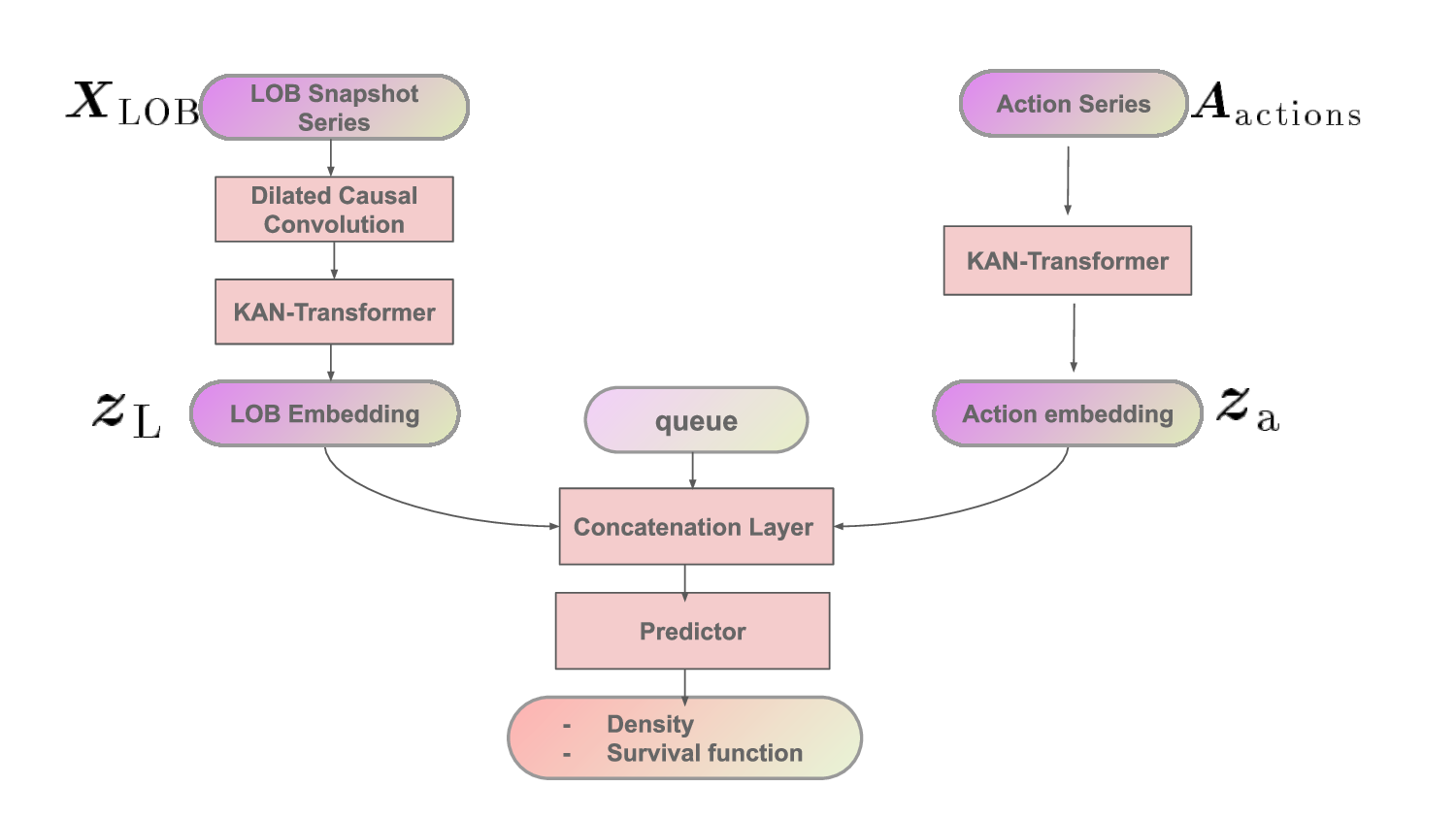
In summary, unlike previous works [Arroyo et al., 2024, Maglaras et al., 2022] that rely solely on a series of LOB snapshots, which may fail to capture the true dynamics of the market as discussed in Section 2.4, our representation integrates three complementary components. First, agent-level signals provide contextual information that helps recover the underlying causes of LOB changes. Second, LOB snapshots capture the state of supply and demand at the moments when these actions are submitted. Finally, queue position reflects the studied order’s execution priority under price-time matching [Huang et al., 2015, Cartea et al., 2014]. These three components are summarized schematically in Figure 2, which illustrates how they are later processed within the KANFormer presented in the next subsection. (4n+4) are processed by a DCC block followed by a KAN-Transformer to produce a LOB embedding. Agent actions Aactions ∈ R L×(d+5) are encoded by a KAN-Transformer to produce an action embedding. The two embeddings are concatenated with the queue position q and passed to the predictor, which outputs density and survival function.

which are then passed to the Transformer self-attention layer. This locally-aware convolutional step provides contextualized features, enabling the Transformer to capture both short-term and long-range dependencies in the LOB time series. The outputs of the Action KAN-Transformer and the LOB KAN-Transformer are then combined with the queue position of the studied order and passed to a Predictor, which produces the survival probability and density prediction.

In principle, one could concatenate all features into a single input matrix R L×N , with N = d + 5 + 4n + 4, and process them through a single KAN-Former encoder. However, we adopt two specialized encoders, namely an Action KAN-Transformer and a LOB KAN-Transformer, to better reflect the heterogeneous nature of the inputs. Agent actions (categorical embeddings and behavioral statistics) and LOB snapshots (price-volume and derived features) exhibit distinct temporal dynamics and statistical properties. Dedicated encoders allow the model to capture these patterns more effectively before combining them with the queue position in the predictor. We now introduce each module of the KANFormer model in Figure 2, the left part corresponds to the LOB KAN-Transformer that processes LOB snapshots series, the right part is the Action KAN-Transformer that processes the action series and the bottom part is the predictor that returns the survival function.

The LOB feature matrix X LOB ∈ R L×(4n+4) represents the snapshot of the LOB observed at the exact moments when the actions are submitted. Each snapshot includes the top five price levels, cumulative volumes on the same and opposite sides, and derived statistics such as volatility, spread, volume imbalance, and time of day (see Appendix C). The LOB KAN-Transformer processes this temporal sequence of snapshots to generate LOB embeddings:

z L = KAN-Transformer(X LOB ).

Action KAN-Transformer The agent action matrix A actions ∈ R L×(d+5) encodes the sequence of event messages before t 0 i . Each row corresponds to an action, described by its type (embedded in R d ) and the five behavioral statistics of the submitting agent. This sequence is processed by the Action KAN-Transformer to produce action sequence embeddings:

Combining LOB, agent actions, and queue position The outputs of the two encoders are concatenated with the queue position q of the studied order, which reflects its execution priority under price-time matching:

Predictor The Predictor maps the combined representation z c to compute the survival function S(t) and the density function f (t), which together determine the likelihood of execution at different horizons. Specifically, we assume that the time-to-fill T of a limit order follows a Weibull distribution 3 . While KANFormer uses KAN-based encoders for representation learning, the predictor assumes a parametric Weibull distribution. Monotonicity of the survival function is guaranteed, ensuring that S(t) is non-increasing, as required in survival analysis.

where λ(z c ) > 0 is the scale parameter and k(z c ) > 0 is the shape parameter. Both parameters are predicted as functions of z c . In practice, we compute log λ and log k for numerical stability [Monod et al., 2024].

The corresponding survival function is:

, 3 Empirically, we found Weibull fit stable and competitive; exploring richer parametric families or discrete-time hazards is left for future work.

which is non-increasing in t, consistent with the definition of survival probability [Kleinbaum and Klein, 1996]. The associated density function is:

.

We analyze the limit order book of front-month CAC 40 index futures contracts. The dataset was provided by Euronext, spanning 300 consecutive trading days from January 6th, 2016 to March 7th, 2017. We focus on orders submitted between 9:05 am and 5:00 pm each day. The dataset is divided chronologically into three subsets. For each subset, the data is generated using the protocol presented in Section 4.1. This split ensures that evaluation is performed strictly out-of-sample.

-Training set: January 6th, 2016 to December 12th, 2016, used to fit the model parameters. -Validation set: December 13th, 2016 to January 24th, 2017, used for hyperparameter tuning and early stopping. -Test set: January 25th, 2017 to March 7th, 2017, held out for final performance evaluation.

Hyperparameters Models are trained with the Adam optimizer [Kingma and Ba, 2014], using an initial learning rate of 10 -3 and apply an exponential learning rate decay schedule with factor γ = 0.9 at each epoch. Training is performed on an NVIDIA RTX A6000 with 48 GB of GPU memory. The lookback window is fixed at L = 50. Hyperparameters are selected by minimizing validation RCLL at 200 epochs with early stopping (patience 10). More details on the grid search are provided in Appendix D.

We train KANFormer by minimizing the negative right-censored log-likelihood (RCLL). test to obtain the four metrics. To ensure stable convergence and reduce computational cost, models M 2 to M 30 were warm-initialized with the parameters of M 1 rather than with random initialization. Warm initialization, which reuses weights trained on a related dataset, has been shown to accelerate optimization and stabilize training in deep learning [Ash and Adams, 2020, Sambharya et al., 2024, Wang et al., 2024]. This strategy ensures that variability across runs reflects only dataset composition, not random initialization effects. We therefore report all results as averages (with standard deviations) over the 30 experiments, providing a controlled quantification of variability in predictive performance.

In summary, KANFormer integrates agent actions, LOB snapshots at the moments of those actions, and the queue position of the studied order into a unified Transformer-based framework enhanced with KANs. This design enables the model to capture market-level dynamics, the drivers of these dynamics and order-level priority, thereby ensuring a well-calibrated and monotonic survival function. In the next section, we evaluate KANFormer on CAC 40 futures data and benchmark it against existing approaches for fill probability estimation.

In this section, we empirically evaluate KANFormer on the CAC 40 futures dataset introduced in Section 4.1. The objective is to assess the model’s ability to predict the survival function of limit orders and compare its performance against existing baselines. We begin by introducing the evaluation metrics and the benchmarks. We then present results from three perspectives: (i) Evaluation metrics and benchmarks, (ii) ablation studies that analyze the impact of input features (Section 3) and architectural choices (Section 4), and (iii) feature attribution analysis, which provides a dynamic view of how feature importance evolves over time.

As introduced in Section 2.3, we evaluate models using both calibration and discrimination metrics. Calibration assesses whether predicted survival probabilities align with observed event frequencies, while discrimination measures how well the model ranks orders by their probabilities of execution. Together, these complementary perspectives provide a balanced assessment of survival prediction quality. We adopt four widely used metrics, here we only present the intuition of theses metrics, formal definitions are provided in Appendix B.

Negative Right-Censored Log-Likelihood (RCLL) RCLL [Balakrishnan andMitra, 2012, Rindt et al., 2022] evaluates the fit of the predicted survival and density functions under censoring. Importantly, RCLL is a proper scoring rule (see Appendix A for a formal definition), which means that in expectation it is uniquely minimized by the true survival distribution. Intuition: A lower RCLL indicates better calibration, i.e., the predicted distributions match the observed outcomes more closely.

Concordance Index (C-index) We use the classical, time-independent C-index [Harrell Jr et al., 1996, Uno et al., 2011]. It provides a global measure of ranking quality by comparing all pairs of orders: a pair is concordant if the order with a higher predicted risk executes earlier. Pairs are comparable only if the earlier event is observed (not censored). In our experiments, we compute a fixed risk score per order as r i = 1 -Ŝ(t * | x i ), where t * is the largest evaluation horizon so that r i aggregates risk over the evaluation window. Intuition: The C-index summarizes overall discrimination across the entire time axis, complementing the horizon-specific information of the AUC.

The Brier score measures the squared error between predicted survival probabilities and observed outcomes at time t [Lee et al., 2019, Graf et al., 1999]. Intuition: It reflects both calibration of predictions; lower values indicate more accurate survival curves. Also, since BS is time-dependent, we report the Integrated Brier Score (IBS) across 20 evaluation horizons chosen between the 10th and 50th percentiles (upper bound is 0.627 seconds) of the event time distribution: IBS = 1 τ2-τ1 τ2 τ1 BS(t) dt, where τ 1 and τ 2 denote the lower and upper bounds of the evaluation window.

The AUC [Lambert and Chevret, 2016] quantifies the model’s ability to discriminate between orders executed by time t (cases) and those still active (controls). Like IBS, we report the average across 20 evaluation horizons chosen between the 10th and 50th percentiles (upper bound is 0.627 seconds) of the event time distribution: IAU C = 1 τ2-τ1 τ2 τ1 AU C(t) dt, where τ 1 and τ 2 denote the lower and upper bounds of the evaluation window. Intuition: A higher AUC at horizon t means executed orders are consistently assigned higher risk than unexecuted ones.

Baselines Following Arroyo et al. [2024], we benchmark our model against MLP, LSTM [Hochreiter and Schmidhuber, 1997], DeepHit [Lee et al., 2018], and LSTM_Hazard [Maglaras et al., 2022]. Note that DeepHit treats survival time as discrete; we linearly interpolate the discrete CDF between bin midpoints to obtain continuous S(t) and f (t). We denote the convolutional-transformer model of Arroyo et al. [2024] as ConvTrans, which uses only X LOB ; ConvTrans ++ extends this baseline with action-type embeddings, agent features, and queue position. We also include two classical survival models: Random Forests (RF) [Ishwaran et al., 2008] and the Cox model [Simon et al., 2011], both implemented with the scikit-survival package [Pölsterl, 2020].

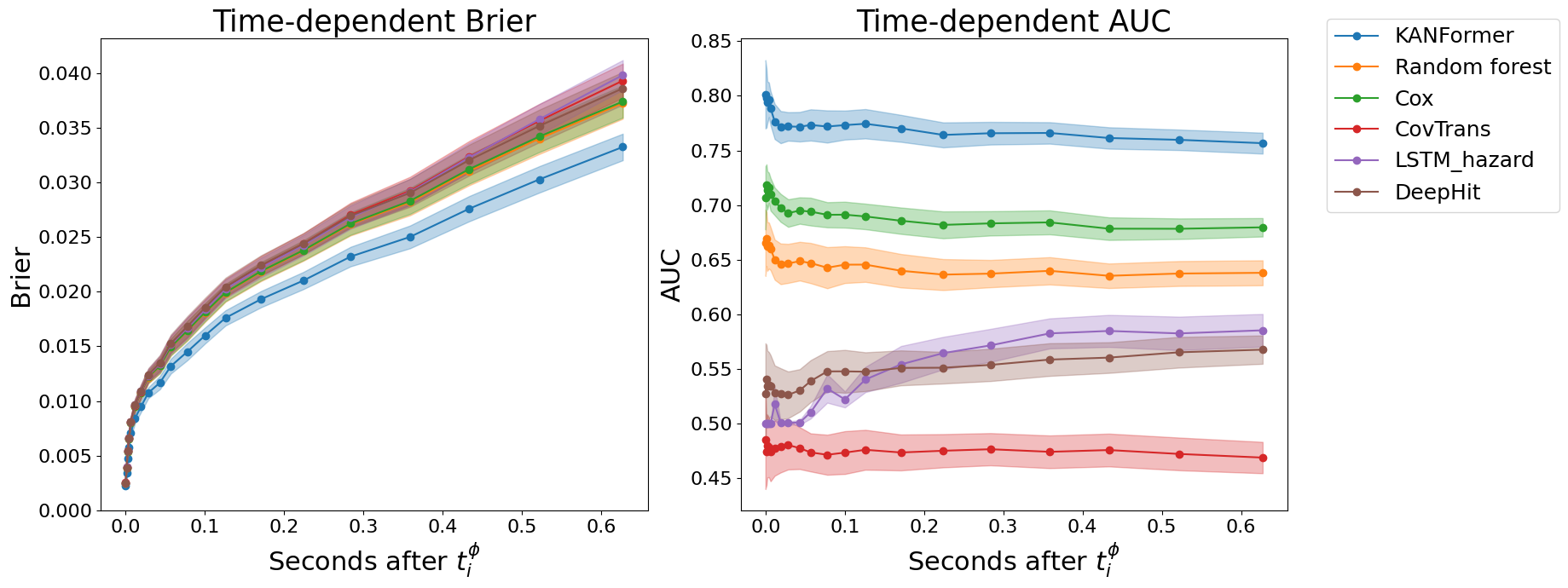
Table 2 summarizes the performance of various models in the limit order book setting. For ConvTrans, only X LOB is used. All other models, including ConvTrans ++ , incorporate action type embeddings, agent features, and queue position. Figure 3 presents the evolution of evaluation metrics over time. Our model outperforms all baselines across all metrics. In terms of calibration, it achieves the lowest RCLL (0.53) and IBS (0.027), indicating highly accurate estimation of the survival distribution. For discrimination, it obtains the highest IAUC (0.76) and C-index (0.72), reflecting superior ability to rank execution risks.

Compared with non-deep models such as Cox and Random Forests, our approach yields substantial improvements in IAUC and C-index, along with better calibration. Among deep learning baselines, ConvTrans, using only X LOB , performs poorly, with near-random discrimination (IAUC and C-index around 0.47). However, ConvTrans ++ shows marked improvements, confirming the importance of including agent-level information and queue position. DeepHit attains relatively strong calibration (RCLL = 0.56, IBS = 0.028), though not as good as KANFormer, but its discrimination is limited (IAUC = 0.56, C-index = 0.58), likely due to its discretized output. In contrast, our model achieves both precise distribution estimation and robust ranking. This demonstrates that accurately modeling fine-grained order dynamics, enriched with behavioral features and queue context, and preserving monotonicity in the survival function, is key to achieving state-of-the-art fill probability estimation.

We now conduct an ablation study to show the impact of model structure and the input features.

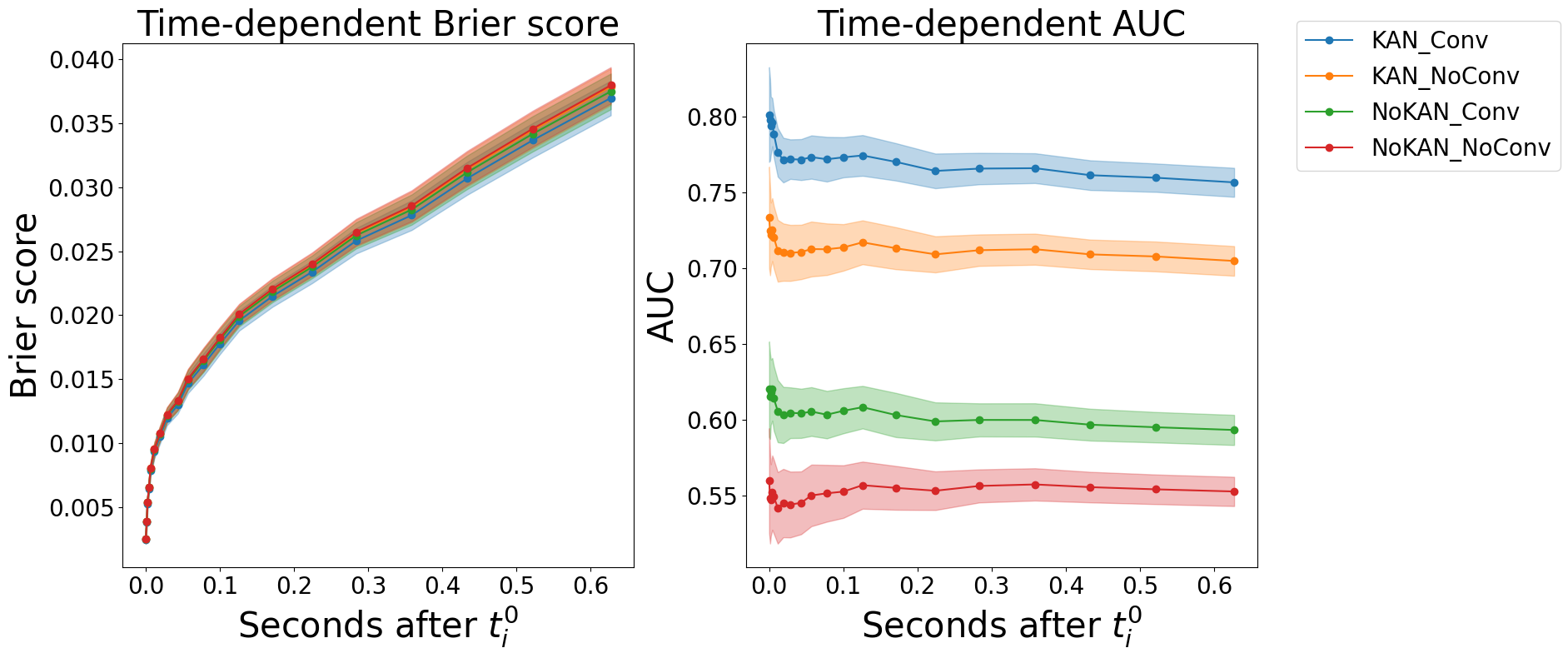
Impact of model structure Table 3 presents an ablation study evaluating the contributions of Kolmogorov-Arnold Networks (KAN) and dilated causal convolution (DCC) to model performance. Across all metrics, the results consistently highlight the benefits of both components. First, comparing KANFormer to its Transformer counterpart, we observe that replacing standard feedforward layers with KAN layers improves both calibration and discrimination. Without convolution, KANFormer improves IAUC from 0.61 to 0.71 and C-index from 0.54 to 0.69. The performance improves further when DCC is added: IAUC increases from 0.63 (Transformer + DCC) to 0.76 (KANFormer + DCC), and C-index from 0.56 to 0.72. These findings support the hypothesis that KAN’s spline-based functional decomposition enhances representation capacity, especially in modeling complex nonlinear dynamics in high-frequency financial environments.

Second, the inclusion of DCC-based convolution improves performance in all cases, demonstrating the importance of capturing local temporal patterns in the limit order book. For KANFormer, adding DCC improves both calibration (RCLL 0.53 to 0.52) and discrimination (IAUC 0.71 to 0.76; C-index 0.69 to 0.72). For the Transformer backbone, DCC primarily improves discrimination (IAUC 0.61 to 0.63; C-index 0.54 to 0.56), while calibration changes little.

Overall, this ablation confirms that the combination of KAN and DCC leads to optimal performance. DCC contributes effective local temporal context, while KAN enhances the functional approximation capacity of the feedforward blocks within the encoders. Together, they result in a highly expressive and wellcalibrated survival model tailored for high-frequency trading applications. As in the previous subsection, we also report the evolution of the Brier Score and AUC in Figure 4.

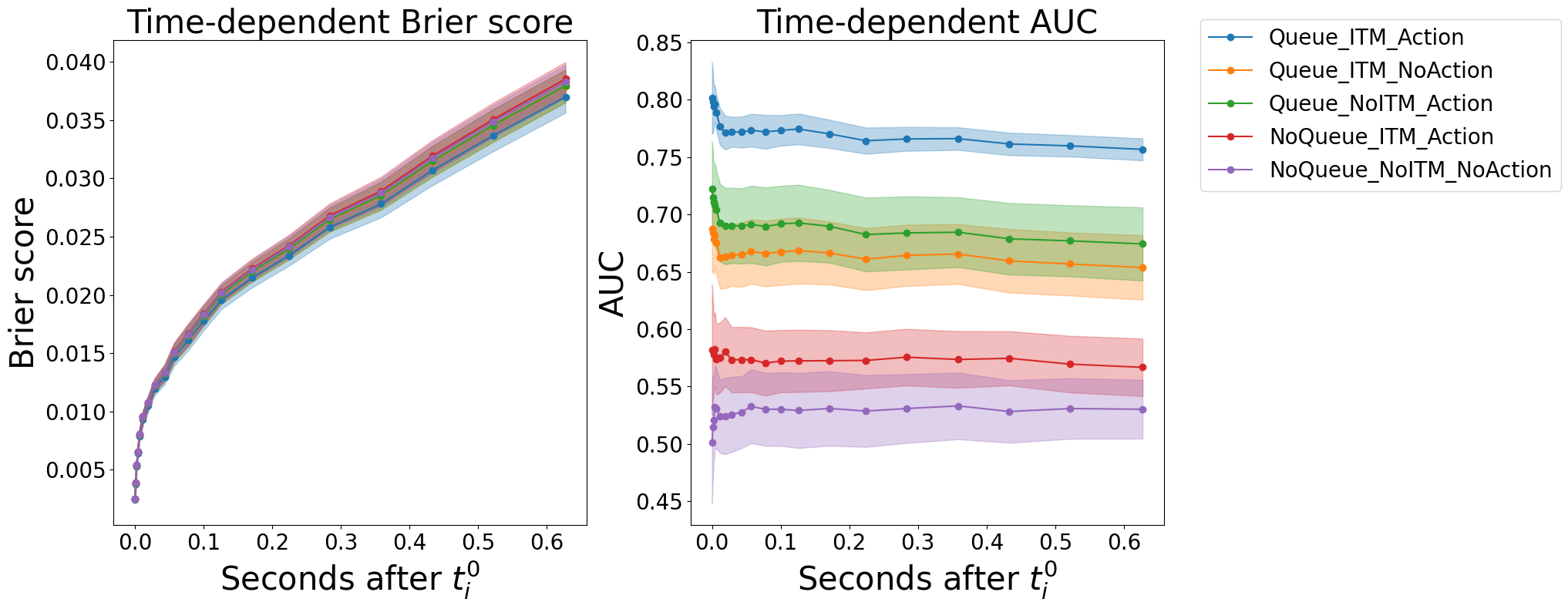
As introduced in Section 4.1, compared to the work of Arroyo et al. [2024], Maglaras et al. [2022], we incorporate additional features into our model, including agent actions (represented by action type embeddings and five representative statistics per agent) and the queue position of the target order. To evaluate the contribution of each feature, we conduct an ablation study using the KANFormer + DCC configuration. Table 4 summarizes the results. In the table, ‘yes’ indicates that a feature is included in the model, while ’no’ indicates its exclusion. The findings clearly show that each feature contributes meaningfully to predictive performance, with the best results achieved when ActionType, Agent Features, and Queue are included.

Excluding the queue information leads to the most substantial decline in performance: IAUC drops from 0.76 to 0.57 and C-index from 0.72 to 0.55. This underscores the critical role of queue position in predicting time-to-fill of limit orders, as it reflects both priority in the order book and local liquidity pressure, two factors essential to accurate fill probability modeling.

Removing agent features also results in notable degradation, albeit less pronounced. IAUC falls to 0.68 and C-index to 0.65, suggesting that agent-level statistics (e.g., Market Ratio, Cancel Ratio) provide valuable insights into the behavioral patterns of market participants. It is important to note that the behavioral statistics of agents, as used in this work, are not observable to a single ActionType AgentFeatures Queue RCLL (↓) IBS (↓) IAUC (↑) C-index (↑) yes yes yes 0.53 ± 0.03 0.027 ± 0.001 0.76 ± 0.02 0.72 ± 0.05 yes yes no 0.54 ± 0.03 0.028 ± 0.002 0.57 ± 0.07 0.55 ± 0.05 yes no yes 0.53 ± 0.02 0.027 ± 0.002 0.68 ± 0.06 0.65 ± 0.06 no yes yes 0.53 ± 0.03 0.027 ± 0.001 0.66 ± 0.06 0.62 ± 0.05 no no no 0.54 ± 0.02 0.028 ± 0.003 0.53 ± 0.07 0.52 ± 0.06 Table 4. Ablation study on input features using the KANFormer+DCC configuration. The table reports performance when including or excluding ActionType, Agent Features, and Queue position as inputs. A value of ‘yes’ indicates inclusion of the feature, while ’no’ indicates exclusion. RCLL and IBS are reported as calibration metrics, while AUC and C-index serve as discrimination metrics. For AUC and BS, results are averaged over 20 evaluation horizons between the 10th and 50th percentiles (upper bound is 0.627 seconds) of the event-time distribution. The C-index is the classical, time-independent version. Reported errors correspond to standard deviations across 30 experiments. Finally, omitting ActionType (while retaining Agent Features and Queue) yields lower performance (IAUC = 0.66, C-index = 0.62). This result indicates that the nature of actions such as insertions, cancellations, or modifications contributes to modeling the evolving dynamics and intentions within the LOB.

Overall, the ablation study confirms that ActionType, Agent Features, and Queue provide complementary and essential information for effective survival analysis of limit orders. This conclusion is also supported by Table 2, it can be seen that the extended model ConvT rans ++ outperforms the baseline Con-vTrans across all metrics. As in the previous subsection, we also report the evolution of the Brier Score and AUC in Figure 5.

In Section 5.3, it has been demonstrated that incorporating ActionType, Agent Features, and Queue information enhances survival analysis for limit orders. While the previous analysis adopted a modular approach by training separate models with different feature combinations, we now focus on a fixed configuration: KANFormer combined with DCC, using all three feature types. Our goal is to illustrate how these features contribute to the model’s predictions over varying time horizons.

To this end, we employ SHAP (SHapley Additive exPlanations) for feature importance visualization [Lundberg and Lee, 2017]. Specifically, SHAP unifies several existing methods under a consistent framework that satisfies desirable properties such as local accuracy, missingness, and consistency [Lundberg and Lee, 2017]. By assigning each feature an importance value representing its marginal contribution to the model prediction, SHAP enables a comprehensive and theoretically grounded understanding of complex model behavior. While KernelSHAP, a widely used variant, provides model-agnostic explanations by estimating Shapley values through sampling, it is computationally intensive, especially for deep learning models with large input dimensions. To address this limitation, we adopt the GradientExplainer provided by the SHAP library, which leverages model gradients to efficiently approximate Shapley values. Gradient-Explainer is specifically designed for interpreting deep learning models, offering a more scalable and practical solution. We leverage GradientExplainer to quantify and visualize the relative importance of features within our KANFormer+DCC model.

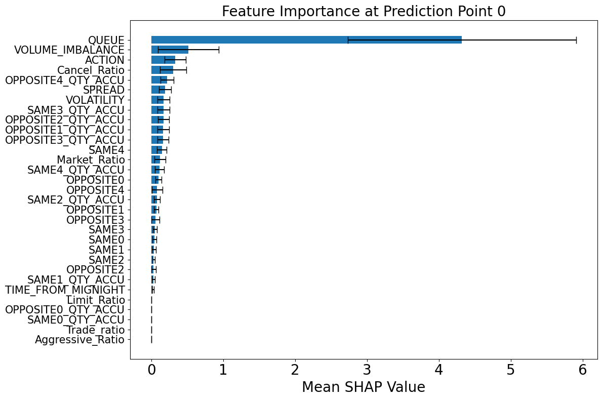
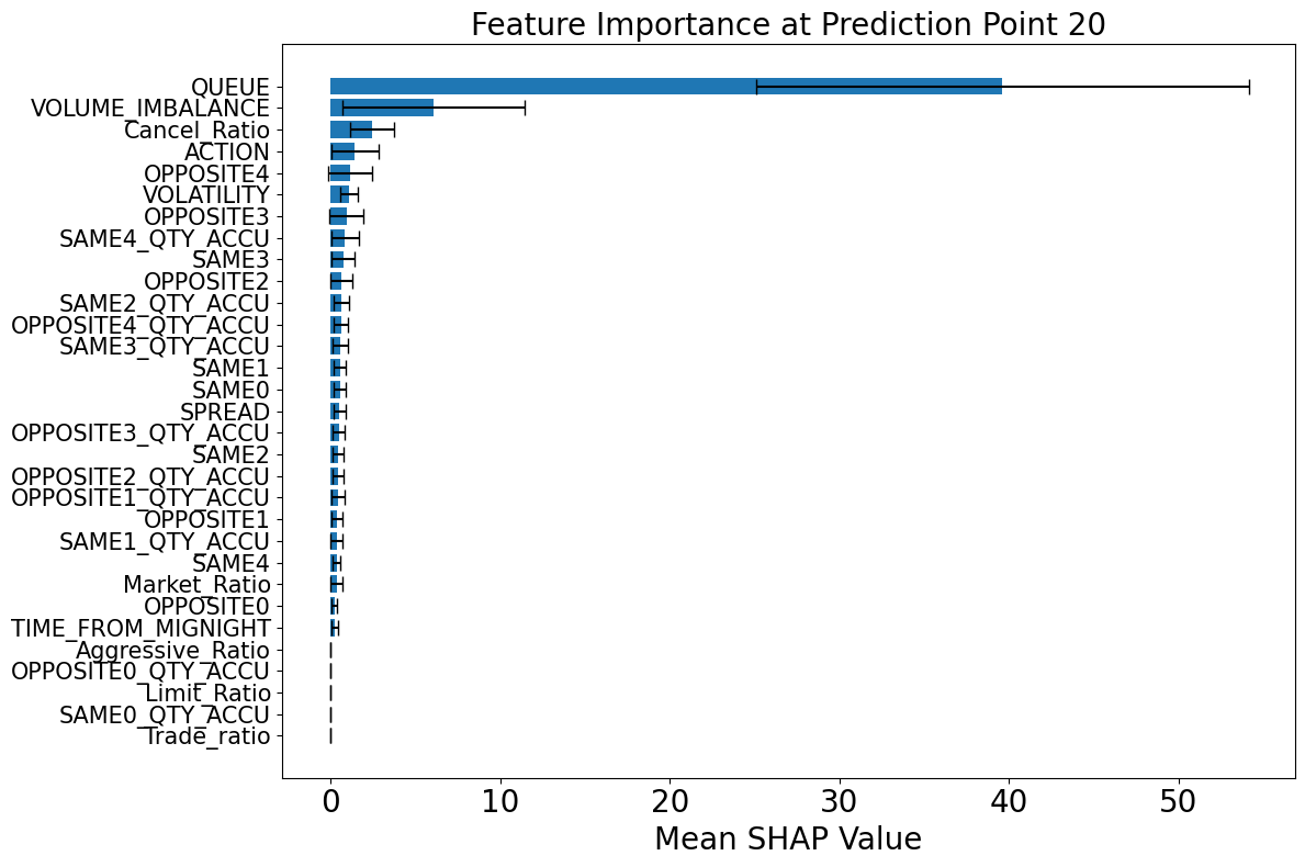
Figure 6 illustrates the evolution of feature importance across various prediction horizons. Notably, the queue position of the studied order emerges as the most influential feature in the short-term horizon, reaffirming its central role in execution modeling, as previously emphasized in the queue-reactive model of Huang et al. [2015] and the microstructural analysis by Cartea et al. [2014]. This is intuitive, as an order’s position in the queue directly determines its priority and likelihood of being matched, especially within short intervals where market conditions are relatively stable.

Volume imbalance also shows consistently high importance across different horizons. As a fast-reacting variable, it encapsulates real-time shifts in demand and supply on both sides of the book. Its predictive power lies in its capacity to capture transient liquidity imbalances, which often precede aggressive trades or cancellations. This aligns with the findings of Arroyo et al. [2024], where volume imbalance was also identified as a top-performing feature in dynamic execution modeling.

The type of action initiated by agents, whether it be an insertion, cancellation, or modification, gains relevance as the prediction horizon lengthens. This trend reflects the growing impact of behavioral signals on execution risk over time. For example, a surge in cancellation actions may indicate a shift in market sentiment or deteriorating order book depth, both of which can adversely affect the fill probability of a pending order. As discussed in Section 2.1, these action types serve as early indicators of directional changes and liquidity shifts.

Among the agent-specific features, the cancel ratio consistently ranks as one of the most informative variables. This metric encapsulates the behavioral tendencies of market participants and helps distinguish between liquidity providers and fleeting liquidity. A high cancel ratio typically signals less commitment to maintaining liquidity, thereby increasing the uncertainty around execution outcomes. Its importance in predicting fill probabilities underlines the value of integrating long-term agent behavior into execution models.

Figure 7 provides a more granular view of SHAP values at two representative prediction times. At earlier time points (e.g., 1.3 ms), the model relies heavily on the queue position and volume imbalance, reflecting a focus on immediate liquidity and priority dynamics. At later prediction points (e.g., 0.627 seconds), the importance of action type and cancel ratio increases, suggesting that the model shifts attention from microstructural immediacy to behavioral messages that reflect evolving market intentions. Collectively, these results demonstrate that the relative importance of predictive features is not static but evolves with the prediction horizon, which is not studied by previous works.

For comparison, Figure 8 shows the evolution of feature importance according to the model proposed by Arroyo et al. [2024], where fast-moving features, such as volume imbalance, are consistently assigned the highest importance.

In this paper, we introduced a new deep survival model specifically designed for predicting the execution risk of limit orders in electronic financial markets. Building on a rigorous survival analysis framework, our model integrates not only the traditional features of the evolving limit order book but also agent-level behavioral features, which capture the dynamics of order flows more comprehensively. Furthermore, by incorporating Kolmogorov-Arnold Networks (KANs) into the Transformer architecture, we enhanced the expressiveness of the model, resulting in improved predictive performance. Our evaluation relied on both discrimination and calibration metrics, providing a holistic assessment of the model’s reliability. Finally, we utilized SHAP to analyze feature importance over time.

Several directions for future research emerge from this work. First, while we have focused on data from the Euronext front-month CAC 40 index futures, it would be valuable to apply our framework to individual equities across different sectors to investigate how execution likelihood patterns vary between asset classes. Such an extension could offer insights into sector-specific market microstructures. Second, while our model directly parameterizes a monotonically decreasing survival function, alternative approaches exist, such as modeling the probability mass function (PMF) or the discrete-time hazard rate [Kvamme and Borgan, 2021]. Exploring these discrete-time modeling strategies, along with their discretization schemes and associated trade-offs, represents a promising avenue for further development. [Arroyo et al., 2024]. The SHAP values are averaged over all orders in the test set.

In Section 5.1, we noted that the negative right-censored log-likelihood (RCLL) is a proper scoring rule, meaning that in expectation the true survival distribution uniquely minimizes the score [Rindt et al., 2022]. This property ensures that RCLL provides a statistically principled measure of model calibration. By contrast, other commonly used metrics such as the C-index and time-dependent AUC (discrimination), or the Brier score and its integrated form, IBS (calibration), are not proper scoring rules. Formally, a scoring rule R takes as input a predictive distribution Ŝ over a set Y, with an observed sample y ∈ Y, and returns a score R( Ŝ, y) ∈ R. With positive scoring rules, higher scores indicate an improvement in model fit.

In survival analysis, a scoring rule R is called proper if, for any true distribution S,

for all predictive survival function Ŝ.

Intuitively, this means that a proper scoring rule incentivizes truthful probabilistic forecasts: the best expected score is achieved when the predictive distribution matches the real distribution. In the context of survival analysis, Rindt et al. [2022] show that RCLL is a proper scoring rule. This implies that, in expectation, the true survival distribution achieves the optimal log-likelihood. By contrast, widely used discrimination metrics such as the C-index or the timedependent AUC, as well as calibration measures like the Integrated Brier Score (IBS), do not satisfy this property. For more details and a formal treatment of proper scoring in survival analysis, see Rindt et al. [2022].

We provide formal definitions of the evaluation metrics used in this paper 4 : AUC, C-index, and Brier Score. Throughout, let {(x i , T C i , δ i )} n i=1 denote the dataset, where T C i = min{T i , C i } is the observed time of order i, δ i = 1 if the order is executed (partially or entirely) and 0 if censored, and Ŝ(t | x i ) is the model-predicted survival function.

For evaluation, we define a time-dependent risk score as

so that higher values correspond to higher predicted probability of execution by time t [Lee et al., 2019].

The AUC at a specific horizon t measures the model’s ability to distinguish between orders that execute before or at t (cumulative cases) and those still active at t (dynamic controls) [Lambert andChevret, 2016, Pölsterl, 2020]. Formally,

, where r i (t) = 1 -Ŝ(t | x i ) is the risk score at horizon t, ω i (t) are inverseprobability-of-censoring weights (IPCW), and I(•) denotes the indicator function. This corresponds exactly to the cumulative/dynamic AUC estimator implemented in Scikit-survival [Pölsterl, 2020]. Intuitively, AUC(t) measures the probability that, at horizon t, a randomly chosen executed order receives a higher predicted risk score than a randomly chosen still-active order.

The concordance index (C) evaluates overall ranking performance across all comparable pairs [Uno et al., 2011]. It is defined as:

.

Here r i is a fixed, order-specific risk score. When predicted risks are identical, 0.5 is counted [Harrell Jr et al., 1996]. Note that the C-index expects a single risk score per order; we therefore define it as the predicted probability of execution up to the largest evaluation horizon t * :

The time-dependent Brier score quantifies the squared error between predicted survival probabilities and observed outcomes at a given horizon t [Graf et al., 1999, Gerds andSchumacher, 2006]. It is defined as:

where I(T C i > t) indicates whether order i is still active at t, and ω i (t) are inverse probability of censoring weights (IPCW) [Pölsterl, 2020]. In experiments, we report the integrated version (IBS), obtained by averaging BS(t) across horizons.

Among the metrics above, only the right-censored log-likelihood (RCLL), introduced in Section 5.1, is a proper scoring rule [Rindt et al., 2022]. This means that, in expectation, the true survival distribution minimizes the score. By contrast, C-index, time-dependent AUC, and the Brier Score are not proper scores and should be interpreted as complementary measures of discrimination or accuracy. For a general discussion of proper scoring rules, see Rindt et al. [2022].

As we present in Section 4.1, the input data for our model is composed of three key sources of information: LOB Features, Agent Actions and Queue position of the order. We now detail the three components.

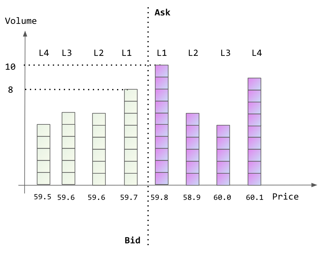
LOB Features: Information from the LOB including top 5 prices, cumulative volumes, and a set of derived statistics. “Same side” is the side of the market that the limit order is submitted to, if the limit order is to buy, the bid side of the market is the same side. The “opposite side” is the other side of the market that the limit order is submitted to, if the limit order is to buy, the ask side of the market is the opposite side. In addition, for the price at each level, we do not use the absolute values. Instead, we use the distance between the price of the corresponding level and the mid price: in ticks. Other predictive patterns include volatility 5 , spread, volume imbalance 6 and time of day. As a result, for each snapshot of a LOB we have 24 features in total to describe the snapshot of the LOB. We illustrate this in Figure 9 with a snapshot of a LOB, where the tick size is 0.1. Suppose that we are studying a limit order at the ask side, and there are 4 units before this order. As such, the same side indicates the ask side; the opposite side indicates the bid side; mid = 59.8+59.7 2 = 59.75. Then the snapshot of the LOB can be described by the vector:

where p l s , v l s , p l o , v l o denotes the price of the same side, the cumulative volume of the same side, the price of the opposite side, the cumulative volume of the opposite side for price level l ∈ {1, 2, 3, 4, 5}. Considering l = 1, p 1 s = 0.5, v 1 s = 10, p 1 o = 0.5, v 1 o = 8; considering l = 2, p 2 s = 1.5, v 2 s = 10 + 6 = 16, p 2 o = 1.5, v 2 o = 8 + 6 = 14, etc.

Agent Actions: The actions of other agents in the market associated with each evolution of the LOB. The action types include:

-I: insertion of a new limit order, -C: cancellation of an outstanding limit order, -R: modification of a limit order that loses priority, r: modification of a limit order that keeps priority, -S: modification of a limit order that becomes aggressive, -T : an aggressive order (market or limit) that is immediately executed, -J: insertion of a stop order. These actions provide contextual insights into the market dynamics. Moreover, we have access to the CAC 40 data from Euronext, we derive 5 representative statistics of the submitting agent, which include Limit Ratio, Market Ratio, Cancel Ratio, Trade Ratio, Aggressive Trade Ratio.

Queue position of the order: The queue position of the order being studied. The LOB features and agent actions can be considered the market context, we also add the queue position of the order being studied. The motivation is 5 Volatility is estimated by computing the rolling average of the squared returns of the mid-price time series over a window of 1,000 trades. 6 Volume imbalance is computed as V I = Vsame-V opposite Vsame+V opposite . Intuitively, a negative V I indicates a stronger opposite side, indicating a higher fill probability and a faster execution of the order, vice versa.

that queue position of the order influences its execution [Huang et al., 2015, Cartea et al., 2014]. Each order is associated with its q, which is used solely in the predictor in Figure 2. For example, for an order being studied, and there are 4 units before this order to be executed, then the queue = 4.

We perform a grid search of hyperparameters over the following ranges:

-Regularization (weight decay): {10 -3 , 10 -4 , 10 -5 } -Batch size: {256, 512, 1024} -Attention heads: {2, 4} -Hidden size: {8, 16, 32} -KAN grid size: {5, 7} -Spline order: {3} -Number of layers: {2, 4, 6} -Dropout rate: {0.1, 0.2, 0.3, 0.4, 0.5} -Action type embedding size: {2, 4, 8, 16}

For the Dilated Causal Convolutions (DCC) applied to LOB snapshots, we fix the kernel size to 3 and the dilation factor to 1, following Arroyo et al. [2024].

In Section 5, we presented the average values of evaluation metrics computed over a set of 20 prediction time points, selected between the 10th and 50th percentiles (approximately 0.627 seconds) of the event time distribution.

As a complementary analysis, Figure 10 shows the evolution of BS, AUC for longer prediction horizons. We observe that as the prediction horizon increases, the performance of most models declines. In particular, AUC values approach 0.5, indicating near-random discrimination. This result is expected: in a highfrequency trading context, a prediction horizon of 120 seconds is relatively long, making it difficult for models to accurately predict survival probabilities and density functions over such extended timeframes. An additional noteworthy finding is that the two non-deep learning baselines, Random Forest and the Cox model, perform better than deep learning models at longer horizons, suggesting that traditional models may offer greater robustness for long-range predictions.

Importantly, our model, KANFormer, achieves higher discrimination performance at short prediction horizons, making it well-suited to high-frequency contexts where timely and precise predictions are critical. This insight suggests applying our model iteratively with short prediction intervals. This strategy ensures that the model operates within the regime where its discrimination ability remains strong, thereby enabling reliable, real-time fill probability estimation.

Note that these agent-level statistics are not available to individual market participants. Therefore, a single agent cannot use the full model discussed in this work.

2 Following[Maglaras et al., 2022], we treat the market symmetrically. “Same side” is the side of the market to which the order is submitted; the “opposite side” is the other side.

📄 Read Full PDF on ArXiv

This content is AI-processed based on open access ArXiv data.