NEAT: Neighborhood-Guided, Efficient, Autoregressive Set Transformer for 3D Molecular Generation

Preprint. January 30, 2026. Generative modeling offers a promising alternative to virtual screening by enabling the computationally cheaper generation of new molecules based on user-defined constraints. Molecular generation can be approached through the generation of (1D) SMILES strings (Kusner et al., 2017;Gómez-Bombarelli et al., 2018), (2D) molecular graphs (Simonovsky & Komodakis, 2018;Cao & Kipf, 2022), (3D) atomic point clouds (Gebauer et al., 2019;Satorras et al., 2021;Hoogeboom et al., 2022;Luo & Ji, 2022;Xu et al., 2023;Daigavane et al., 2024;Zhang et al., 2025;Cheng et al., 2025), or a combination thereof (Hua et al., 2023;Peng et al., 2023;Vignac et al., 2023). Molecules are inherently three-dimensional, with many properties determined by their conformations. While modeling 3D structures is challenging, the additional spatial information is useful for many downstream applications. In this work, we focus on unconditional 3D generation, which is a necessary prerequisite to condition the generation process towards compounds with specific biological functions later on (Peng et al., 2022;Schneuing et al., 2024).

State-of-the-art 3D molecular generation models rely on diffusion and flow matching techniques (Hoogeboom et al., 2022;Xu et al., 2023;Song et al., 2023;2024;Zhang et al., 2025;Feng et al., 2025;Dunn & Koes, 2025). A key limitation of these methods is the need to compute the joint atom distribution at each diffusion step through computationally intensive, quadratically scaling message-passing updates in the encoder model to capture atom interdependencies. Additionally, diffusion and flow matching molecular generators require the number of atoms to be predefined. While the use of dummy atoms offers a partial workaround (Adams et al., 2025;Dunn & Koes, 2025), these approaches remain constrained by the upper bound on the number of nodes sampled from the noise distribution.

Autoregressive models offer a flexible and efficient alternative. They support variable atom counts and require only one encoder call per generated token (Li et al., 2024). For 3D autoregressive molecular generation, there currently exist three lines of work: (1) using graph neural networks (GNNs) in combination with focus atoms (Gebauer et al., 2019;Luo & Ji, 2022;Daigavane et al., 2024); (2) using standard large language models (LLMs) for generating XYZ, CIF or PDB files (Flam-Shepherd & Aspuru-Guzik, 2023) or SE(3)-invariant 1D tokens (Li et al., 2025b;Fu et al., 2025;Lu et al., 2025); (3) combining a causal transformer with a diffusion loss to generate continuous tokens (atomic coordinates) (Cheng et al., 2025;Li et al., 2025a). Although current GNN-based methods ensure permutation invariance with respect to atom ordering, they generate molecules with low chemical validity. Conversely, sequence-based methods perform well in terms of validity but are not permutationinvariant with respect to atom ordering.

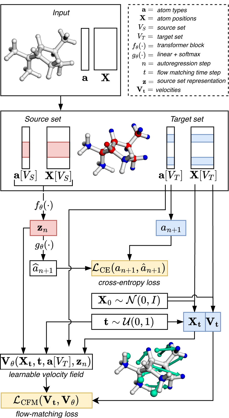
In this work, we present the first autoregressive transformer model for 3D molecular generation that respects the atom permutation-invariance of molecular graphs. Working without canonical atom orderings introduces two challenges. First, it precludes the use of sequence embeddings, which are an essential component of standard autoregressive models. Second, it changes the autoregressive training set-up from supervision with a single token per step to supervision with a set of valid tokens: without a canonical atom order, all atoms in the 1-hop neighborhood of the current graph are valid continuations.

Our solution to these challenges is simple yet effective. Given a partial molecular graph, a permutation-invariant set transformer (Lee et al., 2019) is trained to produce a token distribution that matches the boundary nodes of the subgraph (i.e., all 1-hop neighbors of existing nodes). This training signal, which we refer to as neighborhood guidance, yields a probabilistic next-token distribution without relying on ad hoc canonicalization schemes. We combine it with a flow matching loss to model continuous atomic coordinates.

Our model, NEAT (Neighborhood-guided, Efficient Autoregressive set Transformer), matches state-of-the-art autoregressive 3D molecular generation models on the QM9 and GEOM-Drugs benchmarks while preserving permutation invariance with respect to atom ordering. The permutation invariance enables robust prefix completion without any modifications to the model, yielding unprecedented generation quality.

Autoregressive models generate sequences of tokens by conditioning each token on its predecessors. Formally, given a token sequence x = (x 1 , . . . , x N ), the joint distribution p(x) is factorized as:

where x 1:n = (x 1 , . . . , x n ) represents the tokens up to step n. Sampling is performed by initializing with x 1 and sequentially generating tokens until x N . This is straightforward for sequentially ordered data such as text or images. In the graph domain, the generation order is less obvious, and has been an active focus of research. One way to model graphs as sequences is through canonicalization. However, predefined canonical orderings impose limitations, as the optimal generation order is often context-dependent. To alleviate strict assumptions, You et al. (2018) proposed a breadth-first search node ordering for autoregressive graph generation, while Wang et al. (2025b) introduced order policies to dynamically assign generation orders based on the current state. Although these approaches reduce reliance on fixed orderings, they do not fully eliminate order dependence. 3D molecules are geometric graphs whose structure is determined by connectivity and geometry. The generation of valid positions poses additional constraints on the graph generation process and recent work on this specific task will be discussed in the following.

GNN models with focus atoms G-SchNet (Gebauer et al., 2019) is an E(3)-invariant GNN model that introduces the concept of focus atoms for generation order. In each generation step, the model selects a focus atom as the center of a 3D grid, chooses the next atom type, and infers its position probability from radial distances to previously placed atoms. G-SphereNet (Luo & Ji, 2022) adopts this approach but places atoms relative to the focus atom by generating atom distances, bond angles, and torsion angles with a normalizing flow. The E(3)-equivariant Symphony model (Daigavane et al., 2024) parameterizes the 3D probability around the focus atom using E(3)-equivariant features from spherical harmonic projections rather than rotationally invariant features. While all these models respect the permutation-invariance of atoms, they produce molecules with comparably low chemical validity.

Transformer models with discrete tokenization Transformers can be used for 3D molecule generation when combined with a suitable text format. Flam-Shepherd & Aspuru-Guzik (2023) trained an LLM for 3D molecular generation directly on XYZ, CIF, or PDB files. An active line of research are tokenization schemata to allow LLMs more fine-grained control in the generation process. Geo2Seq (Li et al., 2025b) converts molecular geometries into SE(3)invariant 1D discrete sequences for unconditional modeling, while Frag2Seq (Fu et al., 2025) uses a related technique for structure-based modeling. Uni-3DAR (Lu et al., 2025) employs a voxel-based discretization scheme with an octreebased compression technique, yielding sparse sequences.

Transformer models without vector quantization One of the challenges in generating 3D molecular structures with transformers is to generate continuous-valued tokens like 3D atomic coordinates without discrete tokenization strategies. While standard transformer architectures were initially developed for categorical data, they can be adapted for the generation of continuous values. Li et al. (2024) directly modeled the next-token distribution p(x n+1 | x 1:n ) using a diffusion-based approach, factorized as:

where z n ∈ R k represents an abstract latent variable for the next token. This factorization enables to use a transformer to model p(z n | x 1:n ), capturing interdependencies among tokens, followed by a lightweight diffusion-based multilayer perceptron (MLP) to map z n to the continuous token space.

Their approach enabled high-quality autoregressive image generation with improved inference speed. Cheng et al. (2025) applied this idea to the generation of atomic positions, enabling 3D molecular generation without spatial discretization. They employed a causal transformer with sequential embeddings derived from the atom order in XYZ coordinate files to predict discrete atom types, and a diffusion model, conditioned on these predictions, to predict the corresponding continuous 3D atom positions. However, the study also shows that reliance on a causal transformer introduces limitations. The use of sequence information based on atom order in XYZ files makes the model susceptible to overfitting and degrades performance when the atom order is perturbed. Li et al. (2025a) adopted a comparable framework, adding inertial-frame alignment for coordinates and canonical atom ordering, but their method relocates the problem of token-order sensitivity rather than eliminating it.

We propose that a set transformer (Lee et al., 2019) with bidirectional attention is better suited for autoregressive 3D molecular generation, as it inherently respects the permutation invariance of atom sets by disregarding the generation order of atoms at state n. This raises the challenge of compensating for the absence of sequential order information, which is the key focus of our work.

Overview

A connected graph contains at least one path between any pair of vertices, and a path is defined as a sequence of vertices (v 0 , . . . , v n ) with (v i , v i+1 ) ∈ E for 0 ≤ i < n. The neighborhood of a node index i is the set of all adjacent node indices

we further define the set of boundary nodes

Finally, given a node subset V ′ , we denote the corresponding subset of atom types as a[V ′ ] and the subset of atom positions as X[V ′ ].

Autoregressive 3D molecular graph generation In the build-up phase, the model iteratively predicts atom type a n+1 and position x n+1 , given the current set of atoms and positions at step n. We will use the following compact notation a 1:n = (a 1 , . . . , a n ) to refer to the generated atom types and positions X 1:n = (x 1 , . . . , x n ) at step n. The autoregressive build-up stops when the model predicts a stop token. Edges are then inferred from the N generated atoms via a predefined set of rules like E = R(a, X), which completes inference of the molecular graph G. While edges are inferred from atom types and positions after the buildup phase, the edge information can still be used for teacher guidance in the training phase. In the following, we describe how we use this information for model training.

Neighborhood guidance We propose a sampling strategy that mimics molecular growth during the autoregressive build-up phase. Given a molecular graph G in the training set, we sample a node-induced, connected subgraph

The target set V T is the set of valid token continuations at step n + 1. It is the set of boundary nodes ∂V S , given V S , and induces atom types a[V T ] and positions X[V T ] for model supervision.

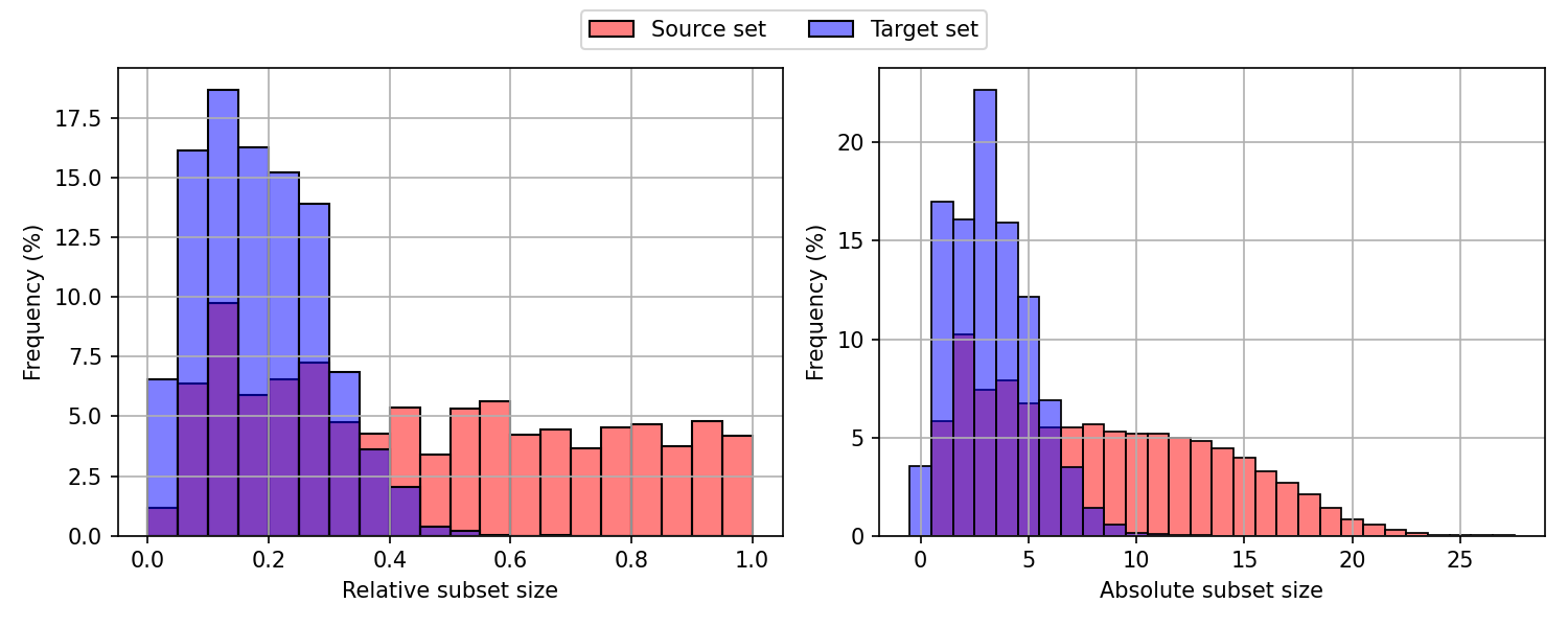
The sampling of connected subgraphs is performed dynamically during training. First, we compute the eccentricity ϵ(v) (the maximum shortest-path distance from v to all other nodes in G) for each node v ∈ V . During runtime, a random seed node v 0 is selected from each molecular graph in the batch. Starting from this seed node, we perform m rounds of 1-hop neighborhood aggregation, where m is a random integer between 1 and ϵ(v 0 ). To avoid biasing the sampling process toward globular subgraphs, we introduce stochasticity by randomly dropping a subset of the boundary nodes in each aggregation round, controlled by a dropout factor γ.

To counteract the resulting bias toward smaller subgraphs, we introduce a scaling parameter β, which adjusts the number of aggregation rounds per graph. By balancing these two parameters, our sampling strategy generates connected subgraphs of varying sizes and shapes, from a single node to the full molecular graph, thereby simulating molecular growth in an autoregressive manner.

The pseudo-code for our sampling strategy is provided in Algorithm 1. Additional information on the impact of γ and β on the sampling strategy and the values used in this work are available in Appendix A.3. In practice, this sampling strategy is efficiently implemented using batched operations and introduces only minimal overhead to the training process, which is dominated by the forward passes through the transformer.

Algorithm 1 Source-Target Split Augmentation

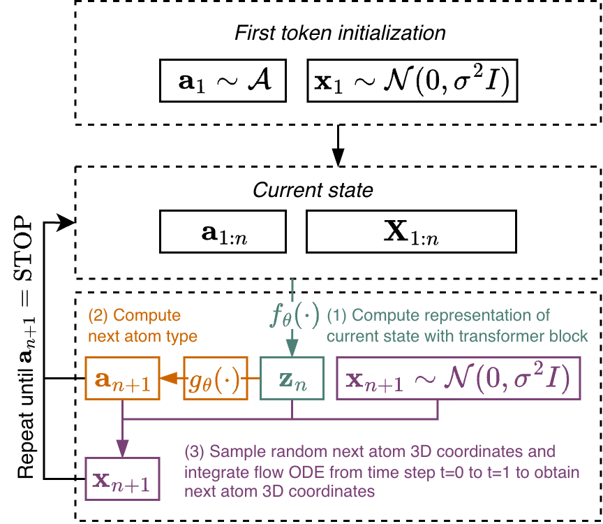
Transformer trunk The computation of the source set representation f θ : (a 1:n , X 1:n ) → z n at step n is straightforward. Atom types a 1:n are encoded using a linear embedding layer, while their positions X 1:n are encoded with Fourier features (Tancik et al., 2020). The summation of these encodings produces the initial node representations. Note that the source set atom positions are not re-centered prior to the computation of the source set representation. For the transformer backbone f θ , we adopt the NanoGPT implementation (Karpathy, 2025) of GPT-2 (Radford et al., 2019), removing positional sequence embeddings and replacing causal attention with bidirectional attention. After the transformer updates, the node representations are aggregated by additive pooling (Zaheer et al., 2017) to form a set-level representation z n , which characterizes the current source set at step n.

The set-level representation z n is used to model the distribution of possible next tokens, represented as the joint distribution p(a n+1 , x n+1 | z n ), which is factorized as follows:

(3) where p(a n+1 | z n ) represents the distribution over the next atom types, and p(x n+1 | a n+1 , z n ) models the distribution over the next atom positions given the next atom type. The next atom type probability p(a n+1 | z n ) is modeled as a categorical distribution over the vocabulary of atom types and is approximated with a linear layer followed by a softmax operation g θ : z n → ân+1 . For model supervision, we compute the cross-entropy loss between ân+1 and the observed distribution over target atom types, which is obtained by computing the mean over the one-hot-encoded atom types in the target set a n+1 = mean(onehot(a[V T ])).

The next atom position is modeled as a conditional distribution given the next atom type. We model this distribution via conditional flow matching (CFM, see Appendix A.1 for a more detailed description of the formalism) (Lipman et al., 2023;Albergo & Vanden-Eijnden, 2023). During training, we employ teacher forcing to decouple the atom type prediction from the task of positional recovery. For the set of possible next positions X 1 = X[V T ] corresponding to the target set V T , we sample a set of random initial positions X 0 ∼ p 0 , where p 0 = N (0, σ 2 I). We construct interpolation paths between the positions at the random position at t = 0 and the true position at t = 1:

with random time steps t ∈ U(0, 1) |V T | , yielding a set of interpolated positions X t with velocities V t = X 1 -X 0 .

We then train the conditional vector field V θ through atomwise regression against the set of CFM path velocities:

F denotes the squared Frobenius norm. The vector field V θ is parametrized with the diffusion transformer (DiT)-style adaptive layer norm (adaLN) MLP from (Li et al., 2024). Input to the MLP for velocity regression is the atom-wise summation of positional encoding, atom type embedding, time step embedding, and the respective source set representation. The final loss is obtained by adding the cross-entropy loss and the flow matching loss.

Distributional coupling and optimal transport In order to reduce the transport cost between the source distribution p 0 and the target distribution p 1 , we employ a simple coupling scheme. Given the positions X 1 and X 0 , we solve the linear assignment problem on the Euclidean distance matrix D(X 1 , X 0 ) and permute the positions in X 0 accordingly. This procedure avoids crossing paths, resulting in improved performance.

Inference The generation process begins by randomly sampling an initial atom type a 1 from the atom type vocabulary A and drawing its initial position x 1 ∈ R 3 from a normal distribution N (0, σ 2 I). At each subsequent autoregressive step, the current atom set (a 1:n , X 1:n ) is passed through the transformer, producing the set-level representation z n . Note that the positions are not re-centered between autoregressive steps. The next atom type a n+1 is predicted from z n using a linear layer followed by the softmax function. A random initial position x n+1 is then sampled from N (0, σ 2 I), and the transport equation is integrated from t = 0 to t = 1 to compute the next atom position (details about the integration scheme are provided in Appendix A.3). This iterative process continues until a stop token is predicted, signaling the end of the molecular generation. The workflow is illustrated in Figure 2. Molecular generation is efficiently implemented using batched operations, enabling parallel generation and high computational speed.

Data We used the QM9 (Ramakrishnan et al., 2014) and GEOM-Drugs (Axelrod & Gómez-Bombarelli, 2022) datasets, detailed information about the data processing is provided in the Appendix A.2. QM9 is a collection of small organic molecules composed of up to nine heavy atoms (carbon, nitrogen, oxygen, and fluorine), with a total of up to 29 atoms when including hydrogen. We obtained the QM9 dataset from Ramakrishnan et al. (2019) and, following standard practice (Hoogeboom et al., 2022;Cheng et al., 2025), randomly split it into training, validation, and test sets, yielding 100,000 molecules for training, 11,619 for validation, and 12,402 for testing after preprocessing. GEOM-Drugs contains 304,313 drug-like molecules, each with up to 30 conformers. Following Dunn & Koes (2025), we loaded the split data from Koes (2024). In line with Vignac et al. (2023), we retained, for each molecule, the five lowest-energy conformers when available. After preprocessing, the dataset contained 1,172,436 conformers across 243,451 unique molecules for training, 146,394 conformers across 30,430 unique molecules for validation, and 146,788 conformers across 30,432 unique molecules for testing. The mean and median number of conformers per molecule are 4.8 and 5.0, respectively. In the following, we refer to GEOM-Drugs as GEOM.

Model training We trained on QM9 for 10,000 epochs and on GEOM for 1,000 epochs, keeping the checkpoint with the lowest total validation loss for inference. Training was done on an NVIDIA RTX Pro 6000 Blackwell GPU with batch sizes of 2048 (QM9) and 512 (GEOM). System specifications, implementation details, and hyperparameters of the final models are provided in Appendix A.3. Appendix A.5 presents scaling analyses with respect to transformer and projection head size. Our best-performing GEOM model employs a 12-layer transformer with 12 heads and hidden dimension 768, and an MLP projector comprising 6 AdaLN blocks with hidden dimension 1536 (165M parameters). This configuration offers a favorable trade-off between generation quality and model size. Our best performing QM9 model (282M parameters) uses a 16-layer transformer with 16 heads and hidden dimension 1024. We speculate that having to use a larger model for the seemingly easier QM9 dataset might be due to the highly constrained molecular geometries of the QM9 dataset, which might need higher model capacity.

To evaluate the quality of generated molecules, we adhere to standard practices (Hoogeboom et al., 2022;Daigavane et al., 2024;Zhang et al., 2025;Cheng et al., 2025) and report atomic stability and molecular stability, validity, uniqueness, and novelty. An atom is considered stable if its valence satisfies the octet or duet rule. A molecule is defined as stable if all of its atoms are stable. Molecular uniqueness is the percentage of distinct canonical SMILES strings derived from valid molecules, or in other words, the percentage of valid and unique designs. Novelty is the percentage of valid, unique designs that are not present in the training set. For all metrics, we generated 10,000 samples and reported the mean value and 95% confidence interval across three runs Molecule building Molecular validity depends on the algorithm used to construct molecules from the 3D clouds of unconnected atoms that are output by most 3D molecular generation models. We assess molecular validity using two approaches: (1) the widespread EDM pipeline (Hoogeboom et al., 2022) based on bond lookup tables, (2) the pipeline introduced by Daigavane et al. ( 2024) and adopted by Cheng et al. (2025), where a molecule is deemed valid if bonds can be assigned using RDKit’s MolFromXYZBlock function and rdDetermineBonds module, which uses the xyz2mol package based on the work of Kim & Kim (2015). A notable limitation of the EDM pipeline is the absence of aromatic bond handling and a high sensitivity to bond lengths (Daigavane et al., 2024), which yields systematically lower scores for valid aromatic structures and thus reduces the informative value of these metrics. We also observed that the output of RDKit’s rdDetermineBonds module depends on the RDKit version. Throughout this work, we use RDKit v2025.9.1. A detailed discussion of limitations arising from these bond-assignment-based evaluation pipelines is provided in Appendix A.4.

Baselines We compare NEAT trained on QM9 to five autoregressive 3D molecular generation models (G-SchNet (Gebauer et al., 2019), G-SphereNet (Luo & Ji, 2022), Symphony (Daigavane et al., 2024), QUETZAL (Cheng et al., 2025), and Geo2Seq (Li et al., 2025b)). The results are reported in Table 1, with additional comparisons to diffusion-based 3D molecular generation models provided in Appendix A.5. We compare NEAT trained on GEOM to QUETZAL and Geo2Seq, since other autoregressive models were not trained on GEOM and report the results in Table 2. Since the evaluation metrics are sensitive to the procedure used to infer bonds from atomic point clouds, including the choice of algorithm, its hyperparameters, and the software’s version, we generated molecules with the source code and model weights of each baseline wherever possible and evaluated them using a unified pipeline. For G-SchNet, G-SphereNet, and Symphony, we used the precomputed XYZ files released by the authors of Symphony (Daigavane et al., 2023) and computed all metrics with our pipeline. For Geo2Seq, we report the metrics from the original publication.

Unconditional generation performance On QM9, NEAT outperformed all autoregressive models in terms of xyz2mol molecular validity, uniqueness, and novelty. NEAT ranked second to QUETZAL on lookup uniqueness, and third on lookup validity, atom stability, and molecular stability. While Geo2Seq achieved the highest scores for atom stability, molecular stability, and lookup validity, it performed poorly on molecular uniqueness, which we regard as the most critical metric for downstream applications such as drug discovery. Valid designs are of limited practical value if they do not span a broad chemical space. Moreover, low molecular uniqueness may indicate overfitting to the training distribution. On the GEOM dataset, NEAT achieved the highest lookup molecular validity and uniqueness. Both QUETZAL and NEAT exhibited complete novelty and similarly low molecular stability, close to that of the GEOM test set (2.8%). Further discussion of this value is provided in Appendix A.4. On the xyz2mol metrics, NEAT underperformed relative to QUETZAL, likely due to differences in objective complexity. QUETZAL employs a standard causal transformer objective, whereas NEAT models the full distribution of token continuations, which introduces substantially higher degrees of freedom and increases the risk of error accumulation during inference. Nevertheless, our approach yields greater robustness in downstream applications, a trade-off examined in the subsequent prefix-completion experiments.

Table 1. Performance comparison of NEAT against autoregressive 3D molecular generators trained on QM9. All metrics are reported as percentages. The first row reports results on the QM9 test set (12,402 molecules). All other rows report results computed from 10,000 generated molecules. The best and second-best entries are shown in bold and underlined, respectively. Entries for which generated molecules could be retrieved to be re-evaluated with our pipeline are marked with a single star (*). Entries for which the source code and model weights were available to generate molecules are marked with two stars (**). For these models and for NEAT, we report the mean and 95% confidence interval over three runs.

Prefix completion A common task in medicinal chemistry is to design molecules around a given core scaffold. We refer to this as prefix completion: given a target core, the model must produce valid completions consistent with that prefix. Existing approaches are poorly suited to this setting. Canonicalization-based methods such as Geo2Seq, cannot continue from arbitrary prefixes, since the prefix must coincide with the first m atoms of the fully generated molecule after canonicalization. This information is unavailable prior to generation. In principle, permutation-invariant GNNs such as G-SchNet could support arbitrary prefixes, but in practice their generative quality is inferior and sampling is slow. Diffusion models such as EDM require special handling, since they assume joint denoising of all atoms. Xie et al. ( 2024) trained a diffusion model specifically for

scaffold completion, but their approach relies on specialized architectural components and a tailored training procedure.

Although Cheng et al. (2025) report that QUETZAL can perform prefix completion, they provide only qualitative results. Moreover, QUETZAL’s performance is sensitive to the atom ordering in the XYZ files used for training. In ablation studies, the authors showed that perturbing this order degrades performance, which is problematic for prefix completion.

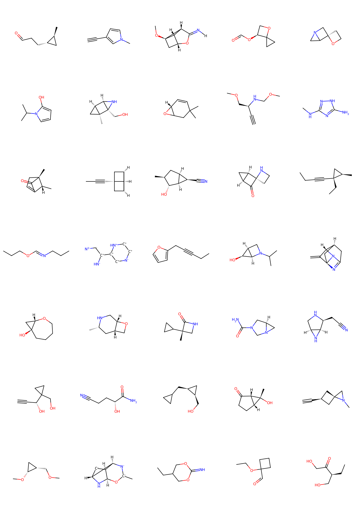
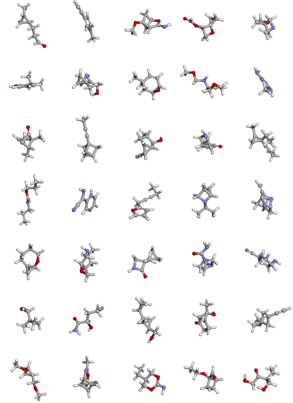
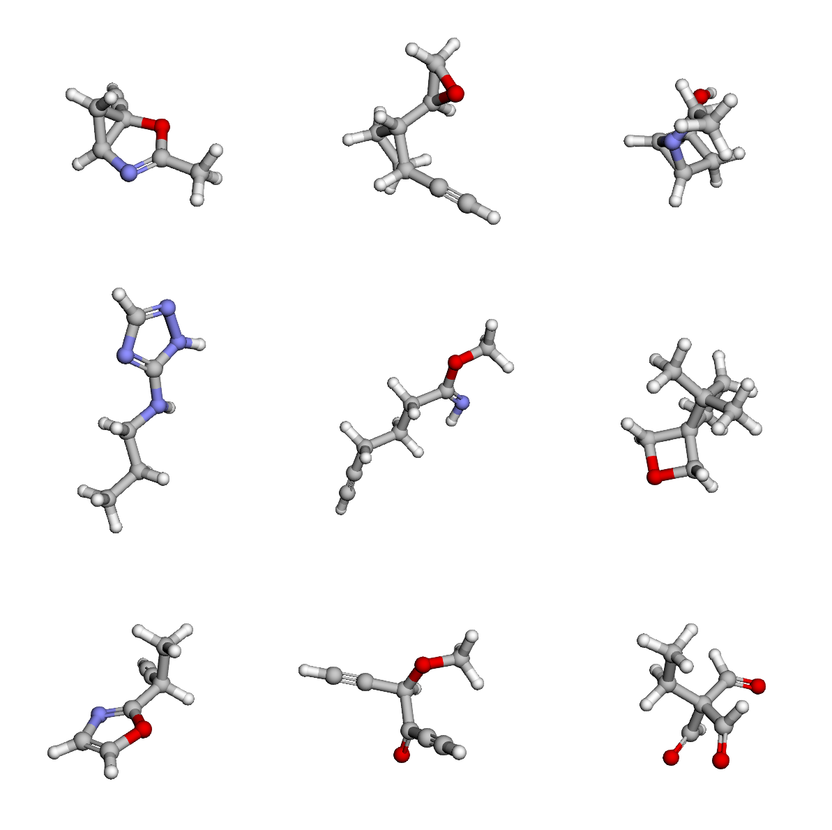
Unlike prior autoregressive models, NEAT enforces atomlevel permutation invariance and avoids sequential posi- tional encodings, which is critical for effective prefix completion. To demonstrate this, we tasked NEAT and QUET-ZAL (trained on GEOM and run with the default settings of the best-performing model) with generating 1,000 molecules from 100 incomplete prefixes automatically extracted from the GEOM training set. These prefixes consist in common ring systems with different substitution patterns. SD files with the 3D atomic coordinates for all prefixes can be found in our code repository and 2D plots are provided in Appendix A.5. Prior to completion, each prefix was randomly rotated and translated for every generated sample. This procedure ensures that repeated generations from the same prefix do not share identical initial atomic coordinates, which could otherwise lead to similar outputs despite the stochasticity of the generation process. As shown in Table 2, NEAT significantly outperforms QUETZAL across all metrics. A summary of the prefix completion workflow as well as randomly selected examples of completed prefixes can be seen in Figure 4.

Runtime Cheng et al. (2025) showed that combining a transformer with a diffusion loss substantially accelerates 3D molecular generation relative to diffusion models. This advantage extends to NEAT. Generating 10, 000 GEOMlike molecules takes 340 s with NEAT versus 712 s with QUETZAL. The runtimes were averaged over three runs on an NVIDIA GeForce RTX 4090 GPU with a batch size of 1000. To maximize comparability, both models use N = 60 integration steps in this comparison.

Limitations NEAT inherits standard limitations of autoregressive architectures. Error propagation might degrade sampling for larger molecules, which could be mitigated by a self-correction mechanism in future work. NEAT produces variable-sized molecules, but does not extrapolate far beyond the maximum atom count seen during training. For large molecules, pooling node embeddings may cause oversquashing and lose key information. Because bonds are not predicted explicitly, bond assignments still rely on predefined rules. Finally, despite random rotations during training, the lack of SE(3) equivariance can yield orientation-dependent predictions.

We introduce a new method for training an autoregressive set transformer with bidirectional attention for 3D molecular generation using neighborhood guidance. Instead of sequential positional encodings, we rely on a subgraph sampling schema for model supervision. Treating the input as a permutation-invariant set removes the need for sequence canonicalization and makes the model well-suited for tasks like prefix completion. On QM9 and GEOM, our approach achieves competitive performance, while offering permutation-invariance with respect to atoms and fast sampling. We believe this provides a strong foundation for future work in conditional 3D molecular generation.

This paper aims to advance the field of machine learning in general, and of de novo molecular design in particular. While we recognize the potential misuse of our approach to generate harmful compounds, we emphasize that there are numerous beneficial applications, such as for instance the development of new pharmaceuticals and safer agrochemicals. Importantly, the generation of molecules is only one step in a complex pipeline, requiring extensive validation, synthesis, and testing before any practical use, which mitigates immediate risks. Furthermore, the ethical deployment of such models should be guided by responsible practices, including rigorous oversight and adherence to safety standards. We do not foresee ethical concerns beyond those generally associated with generative models, but we stress the importance of responsible use to maximize societal benefit while minimizing risks.

A.1. Extended related works Diffusion models for 3D molecular generation Diffusion models (Ho et al., 2020;Song et al., 2021) operate by progressively corrupting the training data with random noise through a forward diffusion process, and training a neural network to reverse this corruption via step-by-step denoising. During inference, new samples are generated by iteratively applying the learned reverse diffusion process to random noise. Prominent diffusion-based molecular generation models include EDM (Hoogeboom et al., 2022), MiDi (Vignac et al., 2023), GeoLDM (Xu et al., 2023), GeoBFN (Song et al., 2024), and SymDiff (Zhang et al., 2025). They have been successfully employed in multiple applications, but they do have notable limitations. First, they require the number of atoms in a generated molecule to be pre-specified, which can be addressed using dummy atom tokens. However, this imposes an upper bound on molecule size. Second, diffusion models use computationally expensive message-passing operations at each step of the stochastic differential equation (SDE) integration to capture atom interdependencies. This results in high computational costs during inference.

Flow matching Flow matching (Lipman et al., 2023;Albergo & Vanden-Eijnden, 2023) offers a conceptually simple alternative to diffusion models and often achieves faster inference due to the need for fewer integration steps during the inference process. It is a simulation-free training framework for generative modeling, where a time-dependent velocity field ψ t is learned to couple a tractable source distribution p 0 with a target distribution p 1 . Typically, p 0 is chosen as a standard normal distribution, p 0 = N (0, I), and the transport is defined over a time interval t ∈ [0, 1]. The transformation of p 0 into intermediate distributions p t is achieved via the push-forward operation #, resulting in a trajectory of probability distributions p t (x t ) at time t. The flow ψ t is modeled using a parameterized function v θ (x t , t), which is trained to approximate the velocity field. Sampling from the target distribution p 1 is performed by drawing samples x 0 ∼ p 0 and integrating the ordinary differential equation (ODE) dx t = v θ (x t , t).

Lipman et al. ( 2023) introduced simulation-free training by constructing conditional probability paths. A widely used choice for these paths is the linear interpolant (Albergo & Vanden-Eijnden, 2023), defined as

The training objective, known as conditional flow matching (CFM), minimizes the l 2 regression loss:

Flow matching-based molecular generation models include EquiFM (Song et al., 2023) and FlowMol3 (Dunn & Koes, 2025). Independent coupling of p 0 and p 1 can result in high transport costs and intersecting conditional paths. These issues can be alleviated by employing optimal transport couplings between the source and target distributions, thereby improving convergence and enhancing flow performance (Tong et al., 2024). In molecular generation, this has been approached, e. g., through rigid alignment of noisy and true coordinates, combined with solving the assignment problem to minimize transport costs (Dunn & Koes, 2025).

The QM9 dataset was retrieved from the figshare repository of Ramakrishnan et al. (2019) and initially comprised 133,885 molecules. The repository additionally provides a list of 3,054 molecule IDs for which OpenBabel failed to infer correct bonds from the XYZ geometry files. Following prior work (Hoogeboom et al., 2022;Cheng et al., 2025), we excluded these molecules. Because the dataset is distributed as XYZ files without explicit bond annotations, and our neighborhood-guidance strategy requires bond information, we reconstructed bonds for each molecule using RDKit (MolFromXYZBlock together with rdDetermineBonds). Bond assignment failed for 6810 molecules, yielding a processed dataset of 124,021 small molecules. We randomly split these into 100,000/11,619/12,402 molecules for the training/validation/test sets, respectively. While some prior works on 3D molecular generation obtained QM9 via the MoleculeNet project (Wu et al., 2018) rather than the original repository (Ramakrishnan et al., 2019), we decided against using the MoleculeNet files. Although they include bond information, the procedure used to determine bonds is not documented, and a non-negligible fraction of molecules in that distribution are charged. This conflicts with the original QM9 specification (Ramakrishnan et al., 2014), which describes the dataset as comprising neutral molecules with up to nine heavy atoms (C, N, O, F), excluding hydrogen atoms.

The GEOM-Drugs dataset was obtained from the FlowMol project’s data repository (Dunn & Koes, 2025) as distributed by Koes (2024). The files provide a predefined train/validation/test split totaling 304,313 molecules, which we adopted unchanged. We removed 35 molecules that failed RDKit sanitization. For molecules comprising multiple disconnected fragments, we retained only the largest fragment by atom count. Following Vignac et al. (2023) where we set m = 0.8 and s = 1.7. With these settings, time steps are sampled more densely around t = 1. We found that this sampling schema slightly improved training above time step sampling from a uniform distribution. For each conditional path, we sampled four random time steps, following Li et al. (2024). Using endpoint parametrization for construction of the conditional paths, like done in Dunn & Koes (2025), led to performance degradation.

Sampling from the flow model We found Euler integration with N = 60 equidistant time steps to be best for integration of the flow ODE for the model trained on QM9 data. We also tried a Runge-Kutta-4 and an adaptive time step Dormand-Prince integrator, but could not find improved performance. For the model trained on GEOM, best results could be obtained by using the Euler-Maruyama integrator, which is described in the following. Sampling from a flow-based generative model can be performed by integrating the ODE dx t = v θ (x t , t) dt. Beyond deterministic sampling, the velocity field can be used to simulate the following reverse-time stochastic differential equation (SDE) (Ma et al., 2024), thereby yielding a stochastic generative model:

where Wt is a reverse-time Wiener process, w t is the diffusion coefficient, and s θ (x t , t) = ∇ log p t (x t ) is the Stein score function. We employ the same Euler-Maruyama integrator as described in Wang et al. (2025a). The score s θ (x t , t) = tv θ (xt,t)-xt 1-t can be derived from the velocity and the diffusion coefficient is calculated as w(t) = 2(1-t) t+η , where η = 10 -3 for numerical stability. In all of our experiments we use τ = 0.3, N = 60 integration steps, and equidistant time step spacing.

Hyperparameters Table 3 and Table 4 summarize the hyperparameters of our best-performing models on QM9 and GEOM. The models have 282M (QM9) and 165M (GEOM) parameters. Results from the hyperparameter screening experiments on GEOM are given in Table 5. The loss function was minimized with the AdamW (Loshchilov & Hutter, 2019) optimizer with parameters β 1 = 0.9 and β 2 = 0.95. We further used gradient clipping to 1.0 of the gradient norm. We implemented a cosine annealing learning rate schedule with linear warm-up epochs and set the minimum learning rate to 10% of the initial learning rate. Model training took 60 and 106 hours on QM9 and GEOM, respectively, given the hardware specifications listed above.

A.4. Observations on evaluation metrics Hoogeboom et al. (2022) introduced a pipeline for generating molecular structures from atomic point clouds by using a look-up table of interatomic distances for single, double, and triple bonds. A bond is established if the interatomic distance is smaller than the corresponding table value plus a defined tolerance margin, starting with the shortest bond type and A notable limitation of this pipeline is that it processes interatomic distances in a sequential manner, which does not guarantee convergence to an optimal solution. Moreover, this pipeline does not consider aromatic bonds, which have lengths between single and double bonds. Consequently, aromatic molecules are often falsely categorized as unstable. For example, evaluating benzene with this pipeline results in 0% atom stability. This occurs because all bonds in benzene are incorrectly assigned as “double” bonds, leading to a chemically invalid configuration where each carbon atom has five bonds (two double bonds to neighboring carbon atoms and one single bond to a hydrogen atom). Given the high prevalence of aromatic compounds in the GEOM-Drugs dataset, this issue leads to a surprisingly low molecular stability on the GEOM-Drugs test set and on the sets of molecules generated from models trained on GEOM-Drugs.

Another peculiarity of the pipeline is that the code used in Hoogeboom et al. (2022) and related works (Vignac et al., 2023;Cheng et al., 2025) reduces all assigned bonds to single bonds when evaluating the GEOM-Drugs dataset. This simplification allows many SMILES strings to pass the RDKit sanitization test, even though they contain carbon atoms with incorrect multiplicities. To ensure fair comparison with other models, we have adhered to this widely used pipeline without modifications.

We also evaluate models using the xyz2mol metric, which tests whether generated 3D atomic point clouds can be converted into valid SMILES after bond assignment via RDKit’s rdDetermineBonds. We would like to point out that this metric is sensitive to the RDKit version used. We observe decreases of up to 5% with RDKit versions later than v2023.3.3, likely due to stricter bond assignment. We use RDKit v2025.9.1 throughout this work, which was the latest available update at project start. We recomputed xyz2mol metrics where model weights or pre-generated samples were available. Literature-reported xyz2mol results with undocumented RDKit versions are marked accordingly. While xyz2mol appears more robust than EDM lookup metrics, we advocate for alternative evaluation pipelines to improve the accuracy and reliability of molecular generator assessment.

Molecular properties of generated molecules We compared the generated molecules to the training set across eight molecular properties: molecular weight, Crippen logP, topological polar surface area (TPSA), ring count, fraction of rotatable bonds, fraction of heteroatoms, fraction of halogen atoms, and fraction of stereocenters (Figure 7). Overall, the distributions of these properties are broadly similar between the two sets. Closer inspection indicates that the generated molecules exhibit slightly broader distributions for molecular weight, logP, and TPSA. The distributions of ring count, fraction of rotatable bonds, and fraction of heteroatoms are slightly skewed toward lower values in the generated set. This skewness is also observed for the fractions of halogen atoms and stereocenters, and is more pronounced for these two properties. Comparison to diffusion models We compare NEAT to six diffusion models (EDM (Hoogeboom et al., 2022), GeoLDM (Xu et al., 2023), GCDM (Morehead & Cheng, 2024), GeoBFN (Song et al., 2024), SymDiff (Zhang et al., 2025), UniGEM (Feng et al., 2025)) in addition to the five autoregressive baselines already discussed in the main body of this work. Regarding QM9, we provide both EDM lookup-table and xyz2mol metrics. For GEOM-Drugs, existing literature primarily reports EDM lookup-table metrics, and uniqueness and novelty are often omitted. Due to the unavailability of pre-trained weights for several baseline diffusion models, we report performance values directly from their original publications rather than performing independent re-evaluations. Consequently, due to this lack of available data, some metrics are missing in our comparison in Table 6. Given the observations discussed in Section A.4, both metrics should be interpreted cautiously. Overall, diffusion models slightly outperform autoregressive models on these benchmarks. Nevertheless, as detailed in the main paper, autoregressive models offer practical advantages like adaptive atom counts, faster inference, and straightforward prefix conditioning.

Prefixes The complete list of prefixes extracted from the GEOM training set is shown in Figure 12, 13, and 14.

Vector field visualization Figures 15-17 illustrate iterative molecular construction by the NEAT model trained on QM9.

Each row corresponds to one construction step. From left to right, panels show Gaussian-initialized points (orange) advected by the NEAT velocity field (gray arrows, with length indicating speed). Trajectories are integrated using explicit Euler with a uniform time step for N = 60 steps. The green diamond marks the point selected as the atom position for the next iteration. We use QM9 for visualization, as examples from the larger GEOM dataset become visually cluttered.

Table 6. Performance comparison of NEAT with diffusion (middle block) and autoregressive (lower block) models trained on the QM9 and GEOM dataset, respectively. All metrics are reported as percentages. The first row reports results on the QM9 and GEOM test set. All other rows report results computed from 10,000 generated molecules. The best and second-best entries are shown in bold and underlined, respectively. Entries for which generated molecules could be retrieved to be re-evaluated with our pipeline are marked with a single star (*). Entries for which the source code and model weights were available to generate molecules are marked with two stars (**). For these models and for NEAT, we report the mean and 95% confidence interval over three runs. Entries marked by a dagger ( †) were taken from Cheng et al. (2025). Metrics for all other entries were taken from the original publications. xyz2mol entries marked with a double dagger ( ‡) are sourced from publications where the RDKit version is either v2023.3.3 or unspecified; these scores may decrease when re-evaluated with RDKit v2025.9.1.

progressing sequentially to larger bond types. If no bond type matches the distance criteria, the atoms remain unbonded. Atom stability within this framework is defined by adherence to the octet or duet rule based on the assigned bonds. Molecular