Uncertainty-Aware Data-Efficient AI: An Information-Theoretic Perspective

Data scarcity fundamentally manifests as epistemic uncertainty. Epistemic uncertainty arises from incomplete knowledge of the true data-generating distribution [5], [6]. Unlike aleatoric uncertainty, which captures irreducible randomness inherent to the data-generation mechanism, epistemic uncertainty can be reduced by acquiring more pertinent training data or by refining model specifications [6].

Uncertainty and information are two sides of the same coin. Information theory provides a rigorous mathematical framework for analyzing and quantifying uncertainty and information [7], [8]. Information-theoretic measures, such as mutual information and relative entropy, have accordingly found extensive application as tools to study data-limited learning. For example, it was shown that the mutual information between model parameters and training data -capturing the sensitivity of the trained model to data -provides bounds on the generalization error of AI models [9], [10].

This review paper covers principles and recent advances on uncertainty-aware AI for data-limited settings from an information-theoretic perspective. The presentation is organized around two complementary strategies for data-efficient AI:

• Quantifying epistemic and predictive uncertainty:

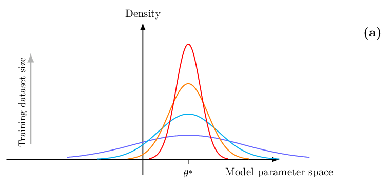
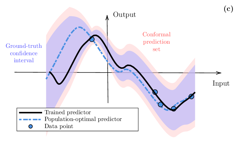
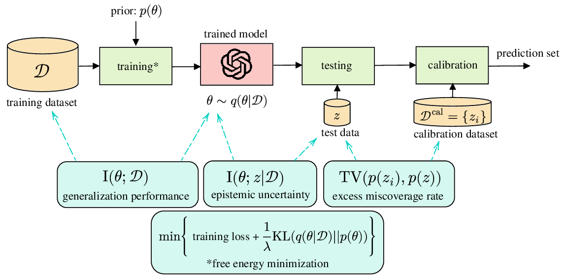
In the presence of limited training data, epistemic uncertainty fundamentally limits the precision of any AI model. Uncertainty quantification is thus an essential step to ensure the reliable deployment of AI models in domains such as robotics, telecommunications, and healthcare. We start by reviewing Bayesian learning as a formal framework to quantify epistemic uncertainty in the parameter space, as sketched in Fig. 1(a) (with θ representing the model parameters). We also cover recent “post-Bayesian” advances including generalized Bayesian learning [11] and martingale posteriors [6], [11]. We then review information-theoretic generalization bounds [9]. As illustrated in Fig. 1(b), generalization bounds offer insights into the scaling of the average error caused by limitations in the training data. As it will be shown, information-theoretic generalization bounds provide a theoretical justification for the use of generalized Bayesian learning. However, these bounds do not provide any actionable quantification of uncertainty for individual inputs. As exemplified in Fig. 1(c), this type of information can be instead obtained via prediction sets calibrated through conformal prediction, which offer distribution-free, finite-sample coverage guarantees [12], [13].

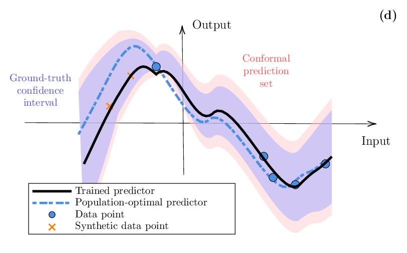
• Leveraging synthetic data: While uncertainty quantification is a required step whenever training data are in limited supply, in practice one may wish to find ways to augment the dataset with additional data. When real data cannot be collected, or is too expensive to obtain, the only remaining option is to leverage synthetic data. This is potentially feasible by leveraging simulators, or digital twins, of real environments [3], [14], [15] or by adopting powerful general-purpose models such as LLMs [16]. As illustrated in Fig. 1(d), synthetic data can be used both to improve training and to enhance the calibration of a pre-trained model. In this context, we review predictionpowered inference, which combines small labeled samples with abundant synthetic predictions for training [17], [18], as well as synthetic-powered predictive inference, which integrates synthetic data for calibration [19], [20].

The remainder of this paper is structured as follows. Section II introduces Bayesian learning and post-Bayesian variants as principled tools to quantify epistemic uncertainty. Section III presents information-theoretic generalization bounds that formalize the trade-off between training data and average accuracy. Section IV surveys predictive methods for uncertainty quantification based on conformal prediction and variants. Section V examines data efficiency via synthetic data through prediction-powered and synthetic-powered inference. Section VI provides concluding remarks and discusses future research directions.

The definition of the information-theoretic measures used in this article is provided in Table I, while Table II reports a table of acronyms. A summary of information-theoretic relationships surveyed in this paper can be found in Fig. 2.

Entropy

Total variation TV(p(a), q(a)) = 1 2 ∥p -q∥ 1

Classical Bayesian inference provides a principled framework for incorporating prior knowledge and quantifying epistemic uncertainty through posterior distributions over parameters affecting the data distribution. The principle can be directly applied to the training of AI models, in which a posterior distribution over the model parameters (denoted as θ) is inferred by combining prior information with a likelihood function [21]. As shown in Fig. 1(a), this leads to a distribution in the model parameter space, whose extent and shape capture the uncertainty arising from the availability of limited data. In practice, the posterior distribution is approximated using sampling, variational methods, or Laplace approximations [6], [22]. The validity of the posterior distribution hinges on the adherence of prior and likelihood to the ground-truth data distribution. However, prior distributions are often chosen for their analytical tractability, and typical likelihood models fail to capture aspects such as outliers [11], [23]. To obviate these issues, so-called “post-Bayes” methods have been introduced. These move beyond conventional Bayesian inference, while retaining the key goal of quantifying epistemic uncertainty. After reviewing conventional Bayesian learning, this section provides a brief introduction to generalized Bayesian learning and martingale posteriors as two important representative post-Bayes frameworks.

In standard Bayesian inference of a parameter θ, one starts by choosing a prior p(θ) and likelihood function p(z|θ), where z represents a data point. In supervised learning settings, the likelihood p(z|θ) takes the form of the conditional distribution p(y|x, θ) with input variables x and output variable y. Given a training set D = {z 1 , . . . , z n }, the posterior distribution is given by

where the proportionality factor is evaluated to ensure normalization. Unlike conventional frequentist learning, which returns a single model parameter θ, the posterior distribution (1) directly quantifies epistemic uncertainty through the spread of probability mass in the parameter space. Wide posterior distributions indicate high uncertainty about which parameters best explain the data, signaling insufficient training samples. As the training dataset grows in size, i.e., in the limit n → ∞, consistency results show that, under appropriate conditions, the generalized posterior concentrates around the optimal parameter θ * , as illustrated in Fig. 1(a). Specifically, the optimal parameter θ * provides the best fit for the true data distribution in terms of the Kullback-Leibler (KL) divergence (see Table I) [24].

Trained predictive or generative models can be obtained by drawing one or more samples from the distribution p(θ|D), typically using Monte Carlo methods [22]. For example, the unadjusted Langevin algorithm produces the sequence of samples

where ξ k are independent standard Gaussian random vectors and η is the learning rate. Iterating the update (2) produces samples that approximate draws from the posterior p(θ|D) as k → ∞ and η → 0 [25]. Note that the update (2) corresponds to a noisy version of standard gradient descent, and that there exist generalizations based on stochastic gradient descent [25] (see also [6]).

With K independent samples θ k ∼ p(θ|D) for k = 1, . . . , K, one can construct the mixture model

which is constructed from the ensemble of models {p(z|θ k )} K k=1 . When the number of samples, K, is sufficiently large, the mixture distribution tends to the true data distribution given the training dataset D,

which is obtained by marginalizing over the posterior distribution p(θ|D). Epistemic uncertainty is captured by the diversity of the ensemble of predictive distributions {p(z|θ k )} K k=1 . In particular, in the case of supervised learning, given an input x, the epistemic uncertainty can be quantified by the degree to which the distributions in the ensemble {p(y|x, θ k )} K k=1 differ from one another.

The diversity of the ensemble, and thus the level of epistemic uncertainty, can be captured by metrics such as the variance of the top-1 predictive distributions {max y p(y|x, θ k )} K k=1 or by information-theoretic measures. A notable such measure is obtained by considering the difference between the entropy of the predictive distribution (4) and the average entropy across the ensemble members, i.e., [6], [26]

where H(z|D) is the entropy of the random variable z ∼ p(z|D) and H(z|θ) is the entropy of the random variable z ∼ p(z|θ). It is emphasized that (5) abuses the conditional entropy notation in Table I, since the dataset D and the parameter θ are fixed (not random) in the entropies H(z|D) and H(z|θ), respectively. The quantity (5) is a measure of the diversity of the distributions {p(z|θ)} obtained by sampling the model parameters as θ ∼ p(θ|D). In fact, the mutual information in (5) equals zero if the distribution p(z|θ) does not depend on θ, and thus the members of any ensemble {p(z|θ k )} K k=1 are minimally diverse, all agreeing with each other. Conversely, the measure ( 5) is large if the distributions p(z|θ) tend to disagree with each other for different samples θ ∼ p(θ|D), yielding more diverse ensembles.

Information-theoretically, as indicated by the notation in ( 5), the difference between the two entropies corresponds to the mutual information I(θ; z|D) between the model parameter and the observation z conditioned on a fixed dataset D (see Fig. 2). This is a measure of the amount of information that we can obtain about the true model parameter θ by observing another data point z, given that we already have access to the dataset D.

We finally note that the mutual information in ( 5) is computed under the assumed prior p(θ) and likelihood p(z|θ). Thus, in order for the conditional mutual information in ( 5) to be a meaningful measure of epistemic uncertainty, one must assume prior and likelihood to be well-specified.

In practice, neither prior nor likelihood are typically guaranteed to reflect the true data-generating mechanism. To improve robustness to such modeling errors, the generalized Bayesian approach supports more flexibility in the specification of the likelihood, as well as in the reliance of the (generalized) posterior distribution on the prior distribution.

To start, the generalized Bayesian methodology replaces the likelihood with a loss-based measure of the fit of model θ for data z. Let ℓ(θ, z) denote such a loss function evaluating parameter θ on data point z. The loss function may, for instance, be the log-loss ℓ(θ, z) = -log p(z|θ), or a generalization thereof that is more robust to the presence of outliers such as the α-log-loss [8], [23], [27]. The training loss is defined as the empirical average of the loss over the training data

The generalized posterior, or Gibbs posterior, is defined as

where the hyperparameter λ > 0 controls the influence of the data relative to the prior. When the loss ℓ(θ, z) equals the log-loss and λ = 1, the Gibbs posterior reduces to the standard Bayesian posterior (1), establishing generalized Bayesian learning as a strict extension of conventional Bayesian learning.

Generalized Bayesian learning can be further extended so as to control the reliance of the generalized posterior distribution on the prior distribution. This is done by observing that the generalized posterior q(θ|D) in ( 7) is the minimizer of the following information-theoretic objective, known as free energy [6], [11]

where KL (•∥•) represents the KL divergence (see Table I). The free energy objective (8) reveals that the generalized posterior distribution arises as a trade-off between fitting the training data, as required by the minimization of the first term in (8), and staying close to the prior, as enforced by the second term in (8) (see Fig. 2).

Replacing the KL divergence with other informationtheoretic divergences, such as the Rényi and Tsallis relative entropies [8], yields a generalized form of the free energy objective (8). The minimizer of this objective represents an extension of the notion of generalized posterior, which has been found to be useful in settings with a misspecified prior [11], [23].

As discussed, generalized Bayesian methods require the specification of a prior and of a likelihood function. However, despite the added flexibility of generalized Bayesian techniques, it may be difficult to identify suitable choices on the basis of the available information about the problem. The martingale posterior approach [28] obviates this issue by requiring only the specification of a predictive distribution, allowing the generation of additional data given the available training dataset. Since there exist powerful foundation models covering a wide variety of data distributions of interest [29], the choice of a suitable predictive model may be practically less problematic than eliciting a prior and a likelihood.

More formally, the martingale posterior reframes posterior uncertainty about parameters as predictive uncertainty on unseen, hypothetical data conditional on the observed data. To model uncertainty over model parameters θ, the martingale posterior specifies a predictive distribution p(D ′ |D) over unseen data D ′ = {z n+1 , . . . , z n+n ′ } given the training data D = {z 1 , . . . , z n }, where n ′ is an integer. In practice, the joint distribution p(D ′ |D) may be specified via one-step conditional distributions via the chain rule

Specifically, in the martingale posterior approach, one draws samples D ′ ∼ p(D ′ |D) of unseen data, and then solves the empirical risk minimization (ERM) problem The connection between samples from the conventional posterior (1) and from the martingale posterior underlying the sequence of samples θ MP in (10) is given by De Finetti’s theorem. Accordingly, if the predictive distribution p(D ′ |D) is exchangeable given D (i.e., if the distribution does not depend on the ordering of the samples D ′ ), the unseen samples D ′ can be conceptually thought of as being generated via the following ancestral sampling scheme:

1. Draw a sample θ from the posterior distribution p(θ|D); 2) Draw the unseen data

In this case, thanks to the consistency of the maximum likelihood estimator, choosing the log-loss ℓ(z, θ) = -log p(z|θ) in (10) ensures that the distribution of the samples θ MP converges in distribution to the posterior p(θ|D) as n ′ → ∞ under weak regularity conditions [28].

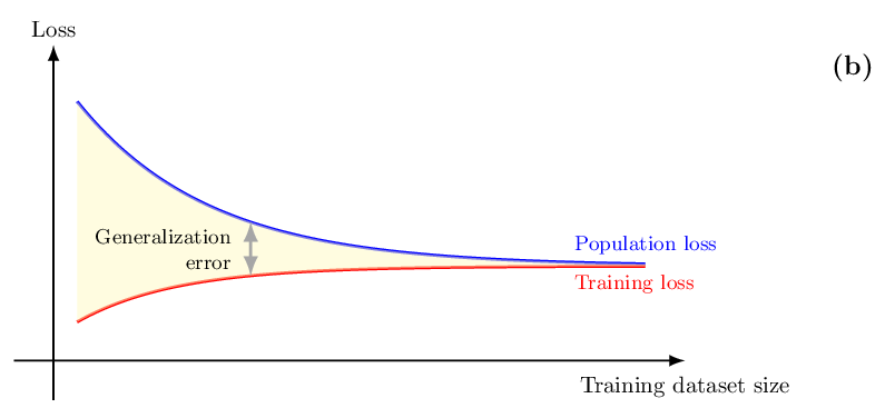
As illustrated in Fig. 1(b), generalization bounds quantify the gap between population loss -the metric ideally minimized during the training of an AI model -and the training loss -the metric actually minimized based on the available data. These bounds provide insights into the training data requirements, potentially offering guidance for algorithm design and data collection strategies. This section briefly reviews generalization bounds that leverage information-theoretic metrics. It will be shown that such bounds provide a theoretical justification for the use of generalized Bayesian learning.

Given a model class, e.g., a class of neural networks, consider a learning algorithm that produces model parameters θ from the training set D = {z 1 , . . . , z n }, where each data point z i = (x i , y i ) is drawn i.i.d. from a given distribution p(z). The trained model parameters θ are typically random functions of the training dataset D. In fact, the output of standard training algorithms such as stochastic gradient descent depends on factors such as random initialization and random mini-batch selection. Furthermore, the generalized Bayesian strategies reviewed in the previous section are often implemented to produce samples θ ∼ q(θ|D) from the generalized posterior, and the martingale posterior, also discussed in Sec. II, generates samples θ via (10).

We denote the conditional distribution of the model parameters given the training data as q(θ|D), so that the trained model is generated as

The distribution q(θ|D) can be, for instance, the generalized posterior (7) or the distribution of the martingale posterior samples (10), but no such restrictions are imposed in this subsection.

To define the generalization error of a training algorithm, with reference to Fig. 1(b), we define the population loss, also known as risk, as the expected value

The population loss represents the ideal target to be minimized via training, and the training loss L train (θ, D) in ( 6) is an unbiased estimate of the population loss. The generalization error is then given by the difference

We are interested in the generalization error gen(θ, D) of the trained model θ ∼ q(θ|D).

Intuitively, as illustrated in Fig. 1(b), the generalization error for model θ ∼ q(θ|D) should decrease as the dataset D grows in size, since the training loss becomes a more accurate estimate of the population loss. In particular, generalization is known to be problematic when the trained model parameters θ exhibit an excessive dependence on the specific realization of the training dataset D -a phenomenon known as overfitting.

Validating this observation, seminal work [30] has shown that, for loss functions satisfying a σ-sub-Gaussian tail condition, the expected value of the generalization error can be upper bounded as

where I(D; θ) represents the mutual information of the random variables D, θ ∼ p(D)q(θ|D). Note that the expected value in ( 14) is also evaluated over the joint distribution of the training data D and of the output of the training algorithm θ ∼ q(θ|D). Accordingly, the mutual information I(D; θ) between the training set and the learned hypothesis quantifies how much information about the random training data is captured by the algorithm’s output (see Fig. 2). Lower mutual information indicates the algorithm produces more stable outputs across different training sets, suggesting better generalization. Extensions of this bound are reviewed in [9]. For specific algorithm classes, such as stochastic gradient descent with appropriate step sizes, the mutual information I(D; θ) grows sub-linearly with n, e.g., as O(log n) [9]. This ensures the right-hand side of the bound ( 14) vanishes as n → ∞, providing theoretical justification for the effectiveness of the corresponding training algorithms in practice. Moreover, the information-theoretic bound ( 14) may also guides algorithm design: techniques like gradient noise injection, dropout, and data augmentation can be understood as mechanisms to reduce the mutual information I(D; θ), thereby reducing the risk of overfitting and hence the generalization error.

It is also possible to derive high-probability upper bounds on the population loss as a function of the training loss, offering another way to bound the generalization error. Specifically, the probably approximately correct (PAC)-Bayes framework yields bounds of the following form. Fix any constant λ > 0; assume that the loss takes values in the interval [0, C]; and choose any prior distribution p(θ) on the model parameter space, as long as it is independent of the training data. Then, for any δ ∈ (0, 1), with probability at least 1 -δ over the random draw of the training set D of size n, the following bound holds [31], [32]

The PAC-Bayes bound (15) quantifies the generalization error via the KL divergence term KL(q(θ|D)∥p(θ)), which provides another measure of the dependence of the trained model on the training data D. With a suitable choice of the prior p(θ) (namely, p(θ) = E D∼p(D) [q(θ|D)]), the average of this term over the training data distribution indeed coincides with the mutual information in (14) (i.e., E D∼p(D) [KL(q(θ|D)∥p(θ))] = I(D; θ)) [9].

The inequality (15) can be rewritten as an upper bound on the population loss, averaged over the output of the training algorithm, as

Since the bound (15), and thus also (16), hold simultaneously for all distributions q(θ|D), the upper bound ( 16) can be optimized over the distributions q(θ|D). This yields a training objective that is closely related to the free energy objective (8).

In fact, both (8) and ( 16) are minimized by the generalized posterior (7). This shows that the generalized posterior distribution is the minimizer of an upper bound on the population loss, justifying its use in settings with limited training data.

While generalized Bayesian learning provides a useful framework for understanding epistemic uncertainty with asymptotic validity properties in the model parameter space, practical deployments often require methods that have finitesample guarantees on the predictive performance in the output space. This section reviews conformal prediction and related techniques that achieve distribution-free uncertainty quantification with minimal assumptions.

Set-valued predictions provide a convenient and actionable way to quantify uncertainty in supervised learning settings. Specifically, given an input x, a set-valued predictor C(x) maps the input to a subset of the output space. For example, in Fig. 1(c), the set C(x) represents the confidence region (error bars) around the trained predictor, shown as the red shaded area. For a desired miscoverage rate α ∈ (0, 1), e.g., 10% or α = 0.1, a useful property for the set predictor is to satisfy the coverage guarantee

where the probability is evaluated over the joint distribution of input x and output y. Accordingly, the true output y is contained within the set C(x) with probability no smaller than 1 -α. When this condition is satisfied, the prediction set C(x) provides quantifiable information about the uncertainty associated with the model’s output. Such insights may enable reliable decision-making in downstream applications. For instance, safety-critical control protocols can ensure that safety constraints hold for any value of the target y within the set C(x), thereby meeting reliability requirements with probability at least 1 -α [33]- [35].

If the ground-truth conditional distribution p(y|x) of the target y given input x were known, the smallest set C(x) satisfying ( 17) could be directly obtained as the highestprobability region under the distribution p(y|x). This optimal set can be expressed as

where the threshold τ (x) is chosen as the smallest value such that the condition

holds, or equivalently,

For discrete output variables y, this set can be constructed by listing the probabilities {p(y|x)} y in non-increasing order for the given input x, and then including in set C * (x) the values of y corresponding to the top elements of this ordered list until the cumulative probability reaches or exceeds the level 1 -α. Importantly, when constructed using the true distribution p(y|x), the ideal set C * (x) satisfies the stronger conditional coverage property

which holds for each fixed value of x. This conditional guarantee is more informative than the marginal coverage in (17), as it ensures the specified coverage level for every individual input x rather than only on average over the input distribution.

The average size of the optimal prediction set (20) can be related to the uncertainty in the conditional distribution p(y|x). Specifically, the average size of the set C * (x) can be bounded in terms of the conditional entropy H(y|x) of the output y given input x [36].

Moreover, considering any fixed input x, one expects that regions of the input space with a higher-entropy distribution p(y|x) yield larger prediction sets. Writing, with some abuse of notation with respect to Table I, as H(y|x) the entropy of the random variable y ∼ p(y|x) for a fixed x, this observation can be formalized as follows. Given two inputs x and x ′ , if the prediction set C * (x) is always larger than the corresponding set C * (x ′ ) for all miscoverage levels α, the probability vector with entries {p(y|x)} y is majorized by the vector {p(y|x ′ )} y [37]. This, in turn, implies the inequality H(y|x) ≥ H(y|x ′ ) between the entropies of the random variables y ∼ p(y|x) and y ′ ∼ p(y|x ′ ) [8], [37].

Conformal prediction (CP) provides a framework for constructing prediction sets with guaranteed marginal coverage (17), regardless of the underlying data distribution [12], [13]. At first glance, ensuring the condition (17) appears to be an impossible goal without knowledge of the true conditional distribution p(y|x). In fact, any trained predictive distribution p(y|x, θ), even when extended to an ensemble as in (3), generally does not match the true conditional probability p(y|x). This discrepancy corresponds to the well-known problem of miscalibration of machine learning models [38]- [40]. Formally, it can, in fact, be proved that it is impossible to ensure the conditional coverage inequality P(y ∈ C(x)|x) ≥ 1 -α, where the probability is conditioned on the input x, unless strong assumptions are made on the conditional distribution of the output given the input [41].

CP bypasses this fundamental limitation by weakening the guarantee to a marginal one: evaluating the probability ( 17) not only over the distribution of the output y, but also over the input x and over calibration data used to evaluate the set C(x). Therefore, from a frequentist perspective, the probability (17) reflects the fraction of realizations of inputs x, outputs y, and calibration datasets for which the target y is found to lie in the prediction set C(x). This requirement can be alleviated in various ways by imposing different notions of partial locality, and the reader is referred to references [42]- [45] for further discussion on this point.

The most computationally efficient variant is split CP. The procedure partitions the available data into training set D and calibration set D cal = {(x i , y i )} m i=1 , and it applies the following steps:

Step 1: Training. Train a model q(y|x) using training set D. Note that the model may be trained using conventional frequentist learning or via Bayesian methods, producing an ensemble predictor as in (3).

Step 2: Evaluate non-conformity calibration scores. Using the trained model q(y|x), compute non-conformity scores s = s(x, y) -henceforth referred to as scores for short -for each (labeled) calibration point (x, y) ∈ D cal . Intuitively, the scores represent the loss (or prediction error) of the pre-trained model q(y|x) on each calibration data point. Evaluating statistics of the calibration scores thus provides insights into the typical behavior of the model. Some examples are provided below.

Step 3: Prediction set construction via score analysis. Given an input x, the prediction set C(x) is constructed by including all the values of y whose score is sufficiently small. Specifically, the threshold is obtained by ordering the calibration scores and evaluating the ⌈(1 -α)(m + 1)⌉-th smallest score. This is denoted as

where s i = s(x i , y i ) is the score for the i-th calibration data point (x i , y i ). As indicated by the notation in (22), this can be equivalently interpreted as the ⌈(1 -α)(m + 1)⌉/mquantile of the empirical distribution of the calibration scores {s 1 , . . . , s m }. Accordingly, for a new test point x, the CP set is evaluated as

Common choices for the scores: Common choices of score function include the following:

• Loss for point predictors: Given the model q(y|x), obtain a point prediction ŷ(x), e.g., as ŷ(x) = arg max y q(y|x), and then evaluate standard loss measures such as the squared loss s(x, y) = (yŷ(x)) 2 for regression. • Conformalized quantile regression score: For scalar regression problems, using the pre-trained model (or models), obtain an estimated α –quantile and an α + -quantile of the conditional distribution of the target y given x, with probabilities α + > α -, which are denoted as qα -(x) and qα + (x), respectively. Then, evaluate the score as [46] s(x, y) = max {q α -(x) -y, yqα + (x)} .

Typical choices for the probabilities defining the quantiles are α -= α/2 and α + = 1 -α/2. • Loss for predictive distributions: For classification, evaluate scores as functions of the probability q(y|x), such as s(x, y) = 1 -q(y|x) or the log-loss s(x, y) = -log(q(y|x)). • Adaptive prediction sets score: Mimicking the ideal prediction set (20), the adaptive prediction set score lists the probabilities as q(y|x) in non-increasing order, and then defines the score as the sum over all target values whose probability is higher than or equal to that for y, i.e., [47] s(x, y) =

• Scores for multivariate target variables: For multivariate target variables, there is a wide range of options that are tailored to the geometry of the target space, with tools ranging from latent-space analysis to optimal transport [48], [49].

In practice, the evaluation of the set (23) depends on the choice of the score. In particular, in some cases, there is an equivalent, computationally efficient formula for the prediction set in (23) that does not require sweeping over all possible values of y. For example, for the conformalized quantile regression score, we have

Theoretical guarantees: The CP set (23) satisfies the desired coverage condition (17) as long as the examples in the calibration dataset D cal and the test pair (x, y) are exchangeable when viewed as a sequence of m + 1 variables. For example, this is the case under the common assumption that calibration data and test data are i.i.d. Importantly, this result holds distribution-free, in the sense that no assumptions on the trained model and on data distribution (besides exchangeability) are required. Consider now a more general situation in which each calibration data point z i = (x i , y i ) has a generally different distribution p(z i ), and denote as p(z) the distribution of the test point z = (x, y). We focus here on the special case of independent data, but the discussion can be extended. Assuming that each calibration data point z i is weighted by a coefficient w i in computing the quantile (22), the coverage property ( 17) is modified as [50]

where TV(•, •) is the total variation distance between two distributions (see Table I). Accordingly, a distribution shift, captured by the total variation distance TV(p(z i ), p(z)), causes an increase in the miscoverage rate beyond the target value α (see Fig. 2). This issue can be mitigated by assigning calibration data points z i with large expected data shifts a smaller weight w i . For example, for a time series, it may be useful to give larger weights to more recent samples.

While standard CP controls the miscoverage rate as in (17), many applications require controlling the expected value of a more general loss function. Conformal risk control (CRC) [51] extends CP to control the expected risk E[L(C(x), y)], where L(C, y) is a loss function that is non-increasing with the size of the prediction set C. CP is recovered by choosing the loss L(Cy) = 1(y / ∈ C), where 1(•) is the indicator function, but other losses supported by CRC include false negative rates in segmentation and tracking [35], [51], as well as rankingdependent error measures [52].

CRC ensures the inequality

where β is a user-specified risk threshold. In a manner similar to (17), the expected value in ( 27) is evaluated with respect to the joint distribution of the test data (x, y) and of the calibration data used to design the prediction set C(x).

The prediction set in CRC is obtained as in (23), with the caveat that the threshold Qα is chosen so as to ensure that the empirical risk m i=1 L(C(x i ), y i )/m over the calibration data does not exceed β plus a slack term dependent on the maximum value of the loss. The procedure generalizes CP.

In practice, it may be more relevant to ensure that the expected risk remains below the threshold β with high probability with respect to the calibration dataset. That is, it may be preferable to ensure the condition

where the inner expected value is with respect to the test pair (x, y), the outer probability is over the calibration data, and δ is a user-defined probability. This goal can be obtained via risk-controlling prediction sets (RCPS) [53], which construct the prediction set by first obtaining an upper confidence bound, with coverage probability 1 -δ, on the expected risk using the calibration data. Then, the threshold in the set ( 23) is evaluated by finding the smallest value of the threshold for which all larger values yield an upper bound no larger than the target β.

The validity of this approach rests on an interpretation of the construction of the prediction set as a form of multiple hypothesis testing. Accordingly, one views the choice of the threshold as the testing of multiple hypotheses, each corresponding to a different choice of the threshold. This principle can be generalized to the optimization of other hyperparameters [54], [55]. In this regard, it is noted that CP can also be described from the perspective of hypothesis testing via the notion of conformal p-values [13].

A fundamental question is: How tight can prediction sets be while maintaining coverage? Intuitively, the answer depends critically both on the generalization error of the model used to evaluate the score functions and on the amount of calibration data available to evaluate the threshold in (22).

In [56], [57], an information-theoretic upper bound on the expected size of CP and CRC sets is derived that takes the form

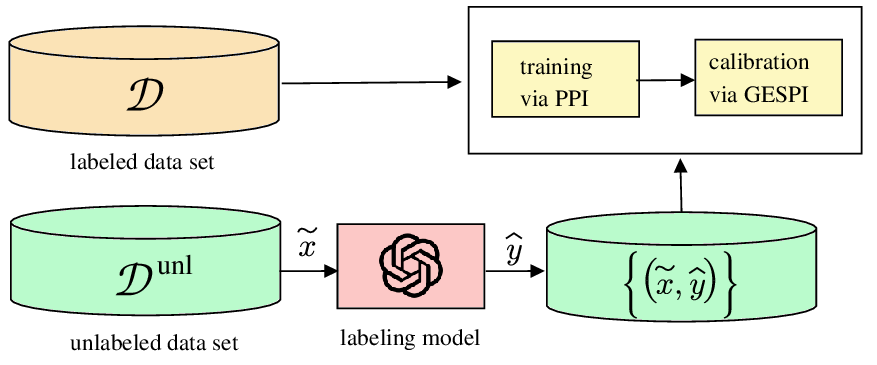
where m is the calibration set size, α is the target miscoverage rate, and gen(θ, D) is the generalization error of the pretrained predictor used to evaluate the scores (see Sec. III). The function f is increasing in the generalization error gen(θ, D) and decreasing in both m and α. This bound shows that reducing generalization error directly improves prediction set informativeness. Furthermore, the bound exhibits an exponential decrease in the calibration dataset size, demonstrating that the demands in terms of calibration data are significantly more limited than in terms of training data. A typical choice is to ensure a number of calibration data points that is of the order 10/α-100/α, growing inversely proportionally with the target miscoverage rate α. Fig. 3. Prediction-powered inference (PPI) [17], [60], [61], and the closely related doubly robust self-training approach [18], [62], integrate synthetic data to enhance model training, while generalized synthetic-powered predictive inference (GESPI) [19], [20] addresses model calibration.

V. DATA EFFICIENCY VIA SYNTHETIC DATA

The previous sections have discussed ways to cope with the availability of limited data through uncertainty quantification. This section covers a complementary approach, whereby the dataset is augmented with auxiliary, synthetic information sources. Examples of this methodology include the use of simulators, or digital twins, of real-world systems to emulate the behavior of the true data distribution. This type of framework is increasingly adopted for practical deployments in the fields of robotics, telecommunications, and healthcare [2], [3]. Other instances of this approach encompass distillation [58] and weak-to-strong generalization [59].

Synthetic data can be potentially used both to augment the training dataset, hence contributing to an improvement of the underlying AI model, and to increase the effective size of the calibration dataset, thus potentially yielding a more accurate quantification of uncertainty. In both cases, the main challenge in using synthetic data is the inherent bias caused by the use of data that does not follow precisely the real-world data distribution. This is also known as the sim-to-real gap when synthetic data are generated by simulators.

This section examines two recent frameworks that address the bias of synthetic data. The first, prediction-powered inference [17], [60], [61], and the closely related doubly robust self-training approach [18], [62], [63], integrate synthetic data to enhance model training, while synthetic-powered predictive inference [19], [20] addresses model calibration.

As illustrated in Fig. 3, prediction-powered inference (PPI) [17], [60], [61] assumes the availability of a small labeled dataset D = {z i = (x i , y i )} n i=1 with true outcomes y i , and a much larger dataset D unl = {(x j )} N j=1 with inputs xj following the same distribution as the labeled dataset, where N ≫ n. The goal is to estimate a vector θ, such as the parameters of an AI model [18], [62], using both datasets to achieve better performance than using labeled data alone.

In PPI, we use an auxiliary labeling model to assign a synthetic label ŷi to each labeled data point (x i , y i ) ∈ D, as well as a label ŷj to each unlabeled data point xj ∈ D unl . Focusing on model training [18], [62], the PPI estimator of the

where λ ≥ 0 is a hyperparameter that determines the extent to which the estimate (30) of the population loss relies on the synthetic labels. It is noted that the PPI estimator (30) relates to prior methods such as doubly robust estimators [64], [65].

Intuitively, the correction term in (30) leverages the true labels to estimate the error caused by the use of the synthetic labels in lieu of the true labels. Note that evaluating this term is possible, since it is computed using labeled data. Thanks to the presence of this correction term, assuming the unlabeled covariates x are drawn i.i.d. from the same distribution of the labeled covariates x, the quantity (30) can be readily seen to be an unbiased estimate of the population loss, i.e.,

where the average is over the labeled and unlabeled data, irrespective of the quality of the synthetic labels and for any value λ ≥ 0. With λ = 1, the variance of the estimator L PPI (θ, D, D unl ) is reduced with respect to the original training loss L train (θ, D) as long as the loss estimate l = ℓ(θ, (x, ŷ)) using the synthetic labels is sufficiently correlated with the true loss l = ℓ(θ, (x, y)) based on the ground-truth labels [17], [18]. Using a Gaussian approximation and denoting as ρ the correlation coefficient between the variables l and l, this implies that the benefits of PPI grow with the mutual information I(l; l) = -log(1 -ρ 2 ).

When this mutual information decreases, by suitably setting the constant λ, one can in principle ensure that the variance of the estimate (30) is never larger than that of the conventional training loss based only on training data [60]. In particular, setting λ = 0 recovers the conventional training loss: L PPI (θ, D, D unl ) = L train (θ, D). A procedure for the online optimization of the hyperparameter λ can be found in [16] (see also [66]).

As seen in Fig. 3, while PPI leverages synthetic labels to enhance parameter estimation, synthetic-powered predictive inference (SPI) [19], and its generalized form general synthetic-powered predictive inference (GESPI) [20], integrate large synthetic data D synth into CP to improve the informativeness of prediction sets when the real, gold standard calibration data D cal is scarce. The synthetic data can originate from various sources, including unlabeled data with pseudolabels, generative AI models, or auxiliary tasks.

The key theoretical guarantee of GESPI is that, under exchangeability of the calibration data, the prediction sets achieve the condition (17) with a slack that depends on the discrepancy between the distributions of the real and synthetic losses, as measured by total variation distance. Importantly, GESPI has an intrinsic guardrail coverage guarantee that holds true even for poor-quality synthetic data, essentially capping the slack total variation term by a user-specified threshold ϵ.

Formally, let C α ′ (x; D) denote the prediction set constructed by CP at miscoverage level α ′ , based on dataset D. GESPI constructs its prediction set as follows:

C GESPI (x) = C α (x; D cal ∪ D synth ) ∪ C α+ϵ (x; D cal ) ∩ C α (x; D cal ). (32) Intuitively, when the synthetic and real data distributions are identical, the prediction set C α (x; D cal ∪D synth ) corresponds to running CP on a larger dataset. This achieves the target miscoverage α, while producing tighter and more stable prediction sets than standard CP.

When the synthetic data is of low quality, the GESPI prediction set (32) ensures bounded miscoverage control through a two-part construction: (i) it takes the union with the guardrail prediction set C α+ϵ (x; D cal ), guaranteeing that the miscoverage is upper bounded by the user-specified α + ϵ level, regardless of how poor the synthetic data is; and (ii) it takes the intersection with standard CP set C α (x; D cal ), deterministically ensuring that the prediction set is never larger than what standard CP would produce.

The benefit of GESPI lies in its improved sample efficiency: when the synthetic data D synth resemble the gold-standard real data D cal , GESPI produces prediction sets with tighter coverage and size than standard CP, especially in the smallsample regime where the calibration dataset size m is limited. Furthermore, regardless of the quality of the synthetic data, the size of GESPI’s prediction sets remains bounded between those of standard CP and guardrail CP applied solely to D cal .

This review paper has discussed information-theoretic foundations and practical methodologies for data-efficient AI. We started by reviewing generalized Bayesian learning as a principled framework for modeling epistemic uncertainty in the parameter space that offers asymptotic validity properties. Information-theoretic generalization bounds were then reviewed as means to formalize the fundamental relationship between data availability and generalization performance, obtaining a theoretical justification for the adoption of generalized Bayesian learning. CP and CRC were presented that deliver distribution-free, finite-sample guarantees on prediction set coverage and general risk metrics, enabling reliable deployment in safety-critical applications. Finally, PPI and GESPI were shown to rigorously integrate auxiliary predictions and synthetic data with limited labeled samples, achieving more effective models and more informative prediction sets while maintaining statistical validity.

In this broad landscape, several promising research directions emerge. Conditional coverage remains an open challenge: while marginal coverage is well-understood, achieving valid coverage conditional on arbitrary covariate subgroups requires either strong assumptions or substantial calibration data [45]. Epistemic uncertainty under distribution shift needs deeper investigation, as current methods struggle to distinguish model uncertainty from environment change [67]. Scaling synthetic data methods to settings such as reasoning in LLM [68] and multimodal models, combining text, images, and sensor data, may require new principled theoretical frameworks. Finally, thorough analyses of real-world deployments of the techniques discussed in this review for robotics, telecommunications, and healthcare would provide further evidence for the importance of uncertainty quantification and synthetic data-based AI training and calibration.

Overall, as AI systems are increasingly deployed in contextspecific engineering applications, the methodologies reviewed here are envisaged to provide essential tools for responsible, data-efficient machine learning. By quantifying epistemic uncertainty and rigorously augmenting limited data, these approaches enable practitioners to navigate the fundamental tradeoff between data availability and predictive reliability.

-THEORETIC MEASURES AND THEIR DEFINITIONS.