A Theoretical Framework for Auxiliary-Loss-Free Load Balancing of Sparse Mixture-of-Experts in Large-Scale AI Models

In modern large-scale AI architectures, s-MoE layers -consisting of several parallel subnetworks (“experts”) controlled by a “sparse gate” or router that selects data to route to them -have largely replaced single submodules through which all data must pass. In these s-MoEs, for each input, the sparse-gating component selects a strict subset of experts (hence “sparse”) to apply to that input. Thus, only a small subcomponent of an AI architecture is activated to process each piece of input data -allowing models to have significantly more parameters while keeping inference and training costs manageable. As a testament to s-MoEs’ utility, recent releases of OpenAI’s GPT (Achiam et al., 2023), Google’s Gemini (Gemini Team et al., 2024), and DeepSeek (DeepSeek-AI, 2025) have all leveraged s-MoE designs to improve efficiency and maintain performance scaling.

However, a crucial aspect of s-MoE design -load balancing (controlling “how many inputs per expert”) -is mostly developed using trial-and-error motivated by heuristic insights (see Section 1.2). Learning to precisely and mathematically balance the load across experts, which reduces monetary losses from idle GPUs, could lead to enormous monetary savings for AI training.

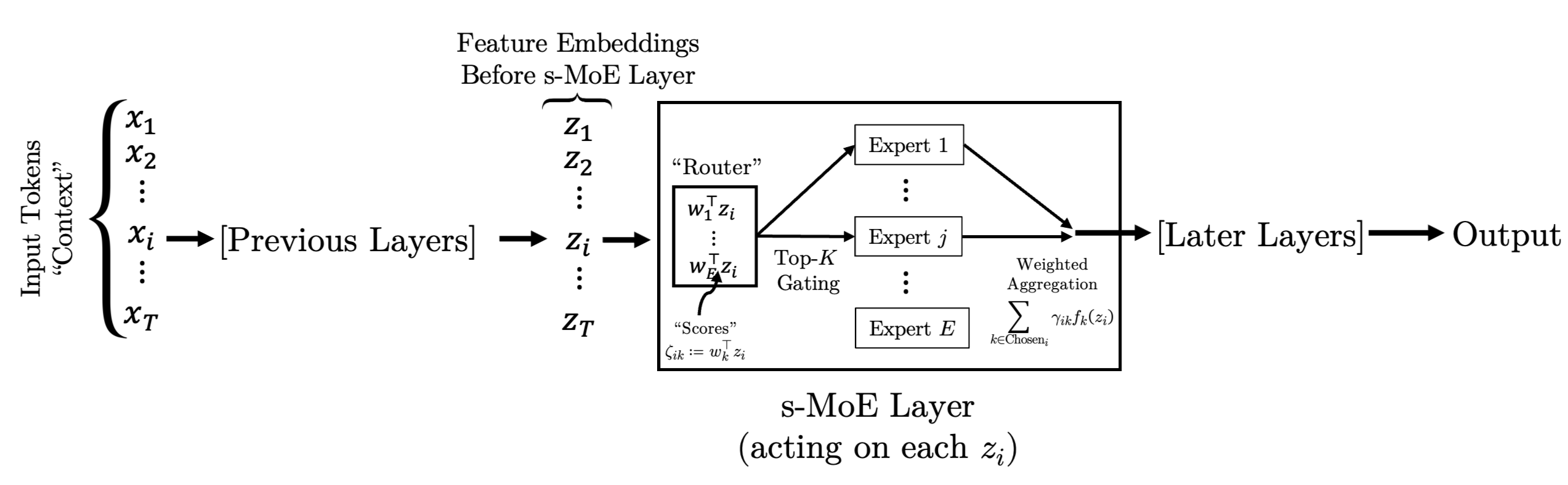
Figure 1 describes the “naïve” setup for s-MoE layers within transformer-based AI models. In particular, the input is a series of token embeddings x 1 , x 2 , …, x T where each x i is a high-dimensional vector corresponding (in language models) to a language unit such as “Hel”, “lo”, “world”, etc. or (in vision models) a patch within an image. Each piece of input data (a sentence, an image patch, etc.) is decomposed into constituent tokens; each token is mapped to its vector embedding x i ; and those embeddings are input into the AI model. The entire tuple of vectors {x i } T i=1 is called the context and T is the context length.

Within the AI model, each of the original token embeddings x i is transformed into feature embeddings by each of the AI model’s layers. In Figure 1, to describe the action of some particular s-MoE layer, we use {z i } T i=1 to denote the feature embeddings before that s-MoE layer.

When a feature embedding “enters” an s-MoE layer with E experts, we calculate an unnormalized affinity score ζ i,k between z i and the k-th expert -usually using an inner product: ζ i,k := w ⊤ k z i . These scores are then normalized, typically using the “softmax” function, into the affinity scores:

The router then selects the Top-K experts based on the K largest γ i,k . The final step in an s-MoE layer is to aggregate the outputs of the selected experts. This is done by computing a weighted sum of the selected experts’ outputs:

where f k represents the k-th expert. Note that the softmax is taken before the Top-K selection, which is typically the preferred order in recent s-MoEs (Dai et al., 2024;Riquelme et al., 2021).

Moreover, the softmax is monotonic, so it is equivalent to choose the Top-K experts based on the K largest {γ i,k } E k=1 for each i. This completes the description of the schematic in Figure 1.

While the naïve routing method of choosing the top-K among {γ i,k } E k=1 is conceptually simple, it could easily cause some experts to idle while others are overloaded. Since GPU time is expensive, such an imbalance could lead to significant monetary losses and inefficiencies in the training process.

Several fixes have been proposed. The most commonly adopted approach is adding an auxiliary “balancing loss” directly to the training loss penalizing the network parameters during training for inducing imbalanced token allocations (Fedus et al., 2022;Lepikhin et al., 2021;Shazeer et al., 2017).

However, this method interferes with the gradient updates of the performance-focused component of the objective (see Section 2.2 of Wang et al. (2024) for a more detailed discussion).

Another approach by Lewis et al. (2021) approximately solves -via a truncated auction algorithm based on Bertsekas (1992) -an integer program that balances the load across experts in every training iteration (corresponding to one mini-batch of data). However, generating an AI model’s outputs for even one single batch of data (a “forward pass”) requires significant computation time and memory since it requires calculating matrix multiplications and non-linear transformations defined by millions to billions of parameters. If this is done during training, there is an additional computational and memory overhead for computing and storing the backpropagated gradients (the “backward pass”). Thus, it is inadvisable to spend additional time solving a multi-iterative subroutine (whether an auction algorithm or an integer program) for every s-MoE layer and every mini-batch.

To address this problem, DeepSeek’s auxiliary-loss-free (ALF-LB) (Wang et al., 2024) procedure augments each expert with a bias p k using a single-shot update (as opposed to a multi-step subroutine), nudging tokens toward underloaded experts -without interfering with training gradients as is done in works leveraging auxiliary balancing losses. Notably, ALF-LB was used to successfully train the recent DeepSeekV3 (DeepSeek-AI, 2024) models.

The ALF-LB procedure (Wang et al., 2024) is as follows:

1. For each expert k = 1, . . . , E, initialize a scalar shift parameter p k to be 0.

2. Perform a forward pass on a mini-batch. During the forward pass, route token i based on the experts with the highest shifted weights γ ik + p k .

3. Calculate the downstream network loss and update the main network parameters, treating the shifts {p k } as constants.

4. For each expert k, update its shift parameter as follows, where u is a small constant (e.g., 0.001):

(2)

5. Repeat steps 2-4 for each mini-batch of input data.

In the original publication, Wang et al. (2024) chose u = 0.001 and exhibited empirical benefits of this procedure on 1B to 3B parameter DeepSeekMoE models (Dai et al., 2024).

Our main contribution is a rigorous theoretical framework for understanding and analyzing the ALF-LB procedure, with specific contributions detailed across different sections. First, in Section 2, we cast the ALF-LB procedure as a single-step primal-dual method for an assignment problem, connecting a state-of-the-art heuristic from large-scale AI to the operations research and primaldual optimization literature for resource allocation such as those in Bertsekas (1992Bertsekas ( , 1998Bertsekas ( , 2008)).

However, the procedure we analyze differs from the aforementioned operations research problems since, as discussed in Section 1.2, the computational and memory requirements of performing a forward pass through an AI model do not allow for one to run multi-iterative procedures as subroutines with those forward passes. Instead, s-MoE balancing routines (such as ALF-LB) must be updated in a “one-shot” manner -with computationally-minimal, constant-time updates per forward pass.

Then, in Section 4, we analyze this procedure in a stylized deterministic setting and establish several insightful structural properties: (i) a monotonic improvement of a Lagrangian objective (Theorem 1), (ii) a preference rule that moves tokens from overloaded to underloaded experts (Theorem 2), and (iii) a guarantee that expert loads converge to a bounded deviation from perfect balance. Finally, in Section 5, we extend our analysis to a more realistic online, stochastic setting by establishing a strong convexity property of the expected dual objective (Section 5.6) and using it to derive a logarithmic regret bound for the ALF-LB procedure (Theorem 13).

It is insightful to compare this paper to another recent line of work at the intersection of AI implementation and operations research: the online resource allocation in AI infrastructures (see Zhang et al. (2024) and citations therein) where computational jobs arrive in an online, stochastic manner at, say, a large data center and must be optimally scheduled to the best server for the job.

In comparison, in the s-MoE balancing problem, for each forward pass, every s-MoE layer must process batches of tokens that all arrive at once. These tokens must all pass through that s-MoE layer before they can collectively move to the next s-MoE layer -an example for reference would be DeepSeekV3 (DeepSeek-AI, 2024), which contains 61 s-MoE layers. Thus, unlike the case studied in Zhang et al. (2024) (Wang et al., 2024), that updates the load balancing parameters with negligible effect on the speed of the forward pass.

We establish a rigorous mathematical framework to understand existing load balancing heuristics, particularly the DeepSeek ALF-LB method. In the remainder of the paper, for simplicity, we will refer to the normalized affinity scores γ ik as the “affinity scores” and adopt the convention of using them both for routing and aggregation.

Consider the exact-balancing primal problem for assigning T tokens to E experts. As a starting point, we make the following assumptions and stylizations:

• The number of tokens multiplied by the sparsity, KT , is exactly divisible by the number of experts E, so the perfectly balanced load is L = KT /E.

• The affinity scores γ ik are constant from iteration to iteration1 .

Hence, the target load is L := KT /E and perfect balance is characterized by the solution of the following integer program (IP):

In practice, it is typically inadvisable (in terms of both time and memory requirements) to solve an IP for every MoE layer and on each individual mini-batch of data2 .

Instead, we first relax the IP to a linear program (LP) by replacing the integer constraint

It is routine to show that the IP and the LP relaxation have the same optimal value. The Lagrangian of the LP relaxation is

The corresponding dual problem is

However, even solving this LP relaxation to completion every iteration would still be too slow and often memory-infeasible.

We show that DeepSeek ALF-LB (Section 1.3) can be formulated as a primal-dual procedure that performs a single-shot update per iteration for finding a critical point of the Lagrangian (4). For conciseness, we introduce the following notation for the load of the k-th expert at iteration n:

ik . Indexing each training iteration with n, consider the following primal-dual scheme:

(5)

Primal Update:

where ϵ

(n) k are step-sizes and TopKInd k ′ (•) gives the indices that would induce the K-largest

to this constraint is equivalent to choosing the top K values of γ ik + p k for each i, regardless of y i .

Thus we can simplify the Lagrangian by dropping the y i terms, which gives:

Within this setup, the original DeepSeek ALF-LB update from Wang et al. (2024) described in (2) corresponds to the step-size 3 Experimental Setup and Observations

In all experiments in this paper (Figures 234), we train 1B-parameter DeepSeekMoE models (Dai et al., 2024) for 100K steps on the next-token prediction task on the Salesforce WikiText-103 dataset (Merity et al., 2016) with the cross-entropy loss. The text data is tokenized using the GPT-2 tokenizer (Radford et al., 2019).

Here, we will provide only a brief description of the DeepSeekMoE architecture for completeness and refer to Dai et al. (2024) for more in-depth details: The DeepSeekMoE architecture follows the paradigmatic practice of stacking decoder-only transformer layers (Vaswani et al., 2017) into a full large language model. In its simplest form, the transformer layer contains several sub-layers -among them a multi-headed attention sub-layer and a multi-layer perceptron (MLP) sub-layer.

For our setting of interest, modern s-MoE architectures (Shazeer et al., 2017;Jiang et al., 2024;Dai et al., 2024) replace the MLP sub-layer of each transformer layer with an s-MoE sub-layer described in Sections 1.1-1.2, where each parallel expert is typically a separate MLP. Additionally, the DeepSeekMoE architecture (Dai et al., 2024) is specifically characterized by its use of “granular segmentation” (using narrower experts but increasing the total number of experts) and the inclusion of two “shared experts” that are always chosen by the gate3 .

The architectural parameters of the 1B-parameter DeepSeekMoE models in our experiments are the same as those described in Wang et al. (2024, Table 5). For consistency with Wang et al.

(2024), we also use E = 64 experts with sparsity level K = 6. During training, we optimize all 1B parameters within the transformer backbone and prediction head of the DeepSeekMoE architectures starting from random initializations. Each model was trained on 8xH100/H200 GPUs with a batch size of 64 sequences/batch and 4096 tokens/sequence (so, T ≈ 262K). To optimize the models, we use the AdamW (Loshchilov and Hutter, 2019) optimizer.

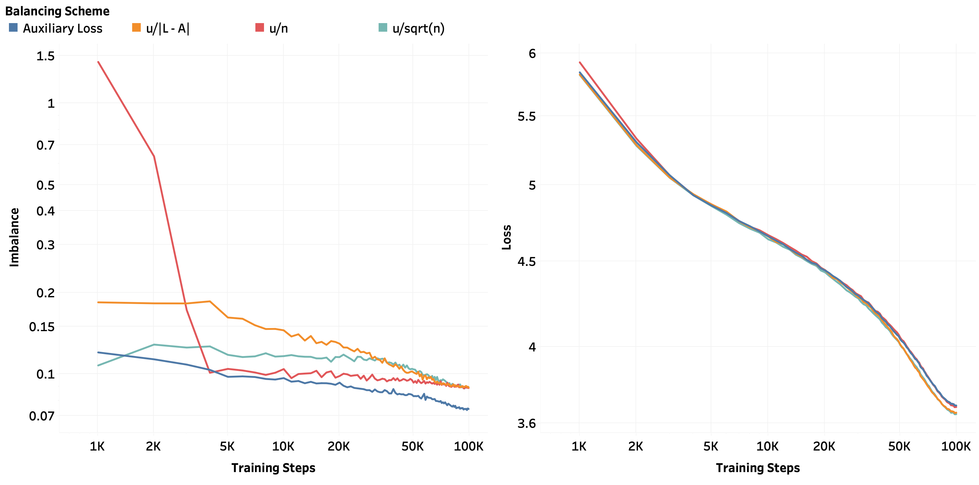
Balancing Schemes. In our experiments, we compare three choices of the k-th expert step-sizes at iteration n (denoted ϵ

2. in the ALF-LB balancing scheme framework. In particular, given some balancing hyperparameter u, we compare the following schemes:

Additionally, we include a comparison with a fourth scheme that trains with an auxiliary loss (Shazeer et al., 2017;Lepikhin et al., 2021;Fedus et al., 2022;Wang et al., 2024). We calculate the auxiliary loss with the method described in Wang et al. (2024, Section 2.2). The auxiliary loss is multiplied by a “trade-off parameter” that we will, for consistency, also denote by u and then added to the main cross-entropy loss.

Hyperparameter Search. For each of the four scheduling schemes, we conducted hyperparameter search over the following hyperparameters:

• balancing constants u ∈ {1e-4, 1e-3, 1e-2, 1e-1, 1, 10},

• learning rates lr ∈ {1e-5, 1e-4, 1e-3}, and

• weight decay wd ∈ {0.01, 0.1, 0.001}.

Thus, we trained 4 × 6 × 3 × 3 = 216 separate 1B-parameter DeepSeekMoE models to conduct this search. Then, for each of the four scheduling schemes, we select the hyperparameter setting that achieves the best cross-entropy loss on a held-out validation set to be shown in the experimental plots and tables in this paper. We found that

• lr = 1e-4 and wd = 1e-1 consistently led to the best validation loss across all settings;

• the u/n and auxiliary loss scheduling schemes performed the best with parameter u = 1; and

√ n scheduling schemes performed the best with u = 1e-3.

We make some interesting empirical observations from our experiments that are of separate interest from the theoretical framework proposed in this paper.

Firstly, we found that, for the original “constant update” scheme considered by Wang et al.

(

k | in our formalization), our hyperparameter search also yielded u = 1e-3 to be the optimal balancing constant, which corroborates the same observation from Wang et al. (2024).

Secondly, Table 1 reports the final validation loss and overall imbalance of the different balancing schemes at the end of training. Observe that the u/ √ n scheme achieves the lowest validation loss (best predictive performance) but the highest imbalance (worst computational efficiency); in contrast, the auxiliary loss approach (Shazeer et al., 2017;Lepikhin et al., 2021;Fedus et al., 2022) achieves the lowest imbalance (best computational efficiency) but the highest validation loss (worst predictive performance). The u/n scheme (which we will analyze in Section 5 through the

To start, we present theoretical guarantees for the convergence of the procedure described by ( 5) and ( 6), assuming fixed scores γ ik . For simplicity, we consider the case where K = 1 for Section 4 only. We will later consider the case where the scores are stochastic and for general K in Section 5.

Towards showing the convergence of this procedure, we will show that the Lagrangian decreases with every iteration. Additionally, we define the assignment function

that gives the assigned expert to token i at iteration n. The switching benefit is defined as

which captures the benefit of switching to expert α n+1 (i) rather than staying with α n (i). Note that b (n+1) (i) ≥ 0 by definition of the primal update.

Theorem 1. (Change in Lagrangian) Using the procedure described in Steps (5)-( 6) (with K = 1), the following holds for the Lagrangian (7):

Proof. By analyzing the change in the two terms of the Lagrangian (7) over one iteration, we have:

This theorem shows that the improvement in the Lagrangian is the difference between the total switching benefit and the squared sum of load imbalances (weighted by step-sizes). We now specialize the analysis to the DeepSeek ALF-LB step-size choice.

Theorem 2. Assume (A) we use the procedure (5)-( 6) with the DeepSeek step-size ϵ

k |, (B) token i switched experts between iterations n and n + 1, and (C) there are no ties in bias-shifted scores. Then, the following must hold:

1. Token i must have switched to a strictly lower designation in the ordering: Overloaded ≻ Balanced ≻ Underloaded.

2. The switching benefit of token i is bounded:

Proof. Since scores are not tied, the switching benefit b (n+1) i must be strictly positive, and

αn(i) > 0. This only happens if token i moves from an expert that is more loaded (relative to L) to one that is less loaded, which

αn(i) , proving (1). The sign difference term is either u or 2u. The bounds in (2) and (3) follow from this observation and the strict inequalities.

Furthermore, letting S (n+1) be the set of tokens that switched experts,

Proof. Follows directly from combining Theorems 1 and 2, and using the strict inequality from the no-ties assumption.

From this, we can show that if the imbalance pattern (which experts are overloaded vs. underloaded) does not “flip” between iterations, the Lagrangian strictly decreases.

Proposition 4. Suppose that at iteration n, a set of experts K 1 has load ≥ L and a set K 2 has load ≤ L. If at iteration n + 1, the same sets of experts remain in their respective loading states (i.e., experts in K 1 still have load ≥ L, and experts in K 2 still have load ≤ L), then

Proof. By Theorem 2, tokens can only switch from an expert in K 1 to an expert in K 2 . This

The result then follows from Corollary 3.

We can reframe the routing decision in terms of preferences. Token i prefers expert k ′ over k at

. Let the score gap be Gγ i k ′ k := γ ik ′ -γ ik and the bias gap be Gp

Proposition 5. Assume two tokens i and j concurrently switched from the same origin expert α n to the same destination expert α n+1 . Then, their score gaps relative to those experts satisfy Gγ i α n+1 αn -Gγ j α n+1 αn < 2u.

Proof. For token i to switch, its score gap must lie in a specific interval determined by the bias gaps:

, where sign_diff is between -2 and -1. The same holds for token j. Since the bounds are independent of the token and the interval has length at most 2u, the result follows.

This proposition implies that if we choose the step parameter u to be smaller than half the minimum difference between any two score gaps, i.e., u < ū where ū = 1 2 min k,k ′ ,i,j Gγ i kk ′ -Gγ j kk ′ , then token movements become unique. Corollary 6. In the DeepSeek implementation, if we choose a constant step-size satisfying u < ū, then no two tokens will move between the same pair of origin and destination experts in two consecutive iterations. As a consequence, an expert’s load cannot change by more than (E -1) tokens between two consecutive iterations.

Proof. A direct consequence of Proposition 5.

Finally, we guarantee that DeepSeek ALF-LB must achieve an approximately balanced state.

Theorem 7. (Guarantee of Approximate Balancing) When applying the DeepSeek ALF-LB procedure using a constant step parameter u < ū, the load of all experts must converge to the range [L -(E -1) , L + (E -1)]. Moreover, once an expert’s load enters that range, it remains in that range.

Proof. If perfect balance is achieved, the shifts p k stop changing and the algorithm terminates.

Otherwise, there will always be an overloaded and an underloaded expert. If an expert k’s load is above L + (E -1), its shift p k will decrease by u each iteration, causing it to shed tokens. By Corollary 6, its load can change by at most (E -1) per iteration. So, its load must eventually enter the range [L, L + (E -1)] without overshooting below L. A symmetric argument holds if an expert’s load is below L -(E -1). Once an expert’s load enters the range [L -(E -1), L + (E -1)], it cannot escape. For example, if an expert’s load is L + j for 1 ≤ j ≤ E -1, it is overloaded and can only lose tokens. It can lose at most E -1 tokens. So its load will remain above L + j -(E -1), which is greater than L -E. A similar argument holds for underloaded experts. Therefore, all expert loads will enter and remain within the stated range.

When the number of tokens is much larger than the number of experts (T ≫ E), the deviation of (E -1) from the perfectly balanced load L = KT /E is negligible. This completes the theoretical demonstration of why the DeepSeek ALF-LB procedure leads to the desirable balancing behavior seen experimentally.

In practice, the affinity scores γ (n) ik evolve during training. Thus, in this section, we generalize the previously considered Lagrangian (7) by assuming that the scores γ (n) ik are stochastic and drawn from expert-dependent distributions. In particular, at iteration n, we assume a random affinity score γ (n) ik ∈ (0, 1) is observed for each token i ∈ {1, . . . , T } and expert k ∈ {1, . . . , E}. The algorithm updates a shift vector p (n) ∈ R E and, for each token i, selects the K experts with the largest values of γ

k is the k-th coordinate of p (n) . Using the notation of Section 2.2, we note that this section will consider a step-size choice of Wang et al. (2024). This is because, when affinity scores become stochastic and time-varying, analyzing the coordinate-dependent u/|L -A (n) k | step-size sequence becomes technically intricate. In contrast, the diminishing and coordinateindependent u/n step-size connects directly with ideas from online convex analysis (Hazan, 2016, Section 3.3.1) leading to cleaner theoretical insights. This adjustment maintains experimental relevance and practicality: Figure 2 and Table 1 demonstrate that using the u/n step-size is comparable in effectiveness as using the original u/|L -A (n) k | step-size. In fact, Table 1 shows that the u/n step-size leads to a slightly better load balancing performance than the u/|L -A (n) k | step-size at the cost of a slightly higher validation loss.

For any vector z ∈ R E , define TopKInd(z) ⊆ {1, . . . , E} to be the set of indices of the K largest coordinates of z with ties broken arbitrarily. For round n and token i, denote Γ (n),i :=

Routing at round n sends token i to the experts in TopKInd Γ (n),i + p (n) . Fix an integer K ∈ {1, . . . , E}. We frame this as minimizing the per-round online loss, which corresponds to the dual online objective:

where L := KT /E is the desired per-expert load for Top-K routing. The k-th component of the

where

counts the number of tokens for which expert k lies in the per-token Top-K set under shifts p. The online dual update corresponding to (5) can then be rewritten as p

k (p (n) ).

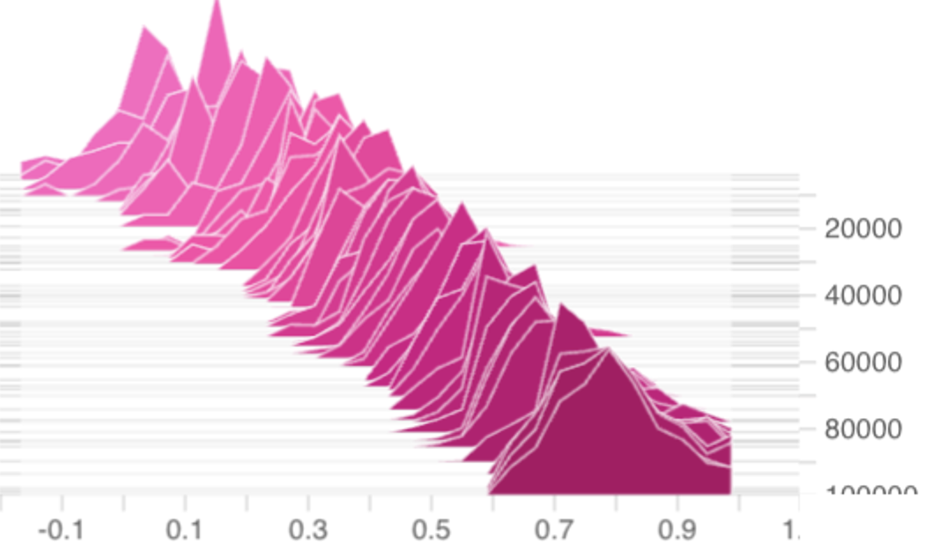
Assume each affinity γ

ik , for a fixed expert k, is drawn independently4 from a distribution that • depends only on the expert k,

• has bounded support on (0, 1), and • has a probability density function (pdf) φ k that is upper bounded by some expert-independent constant. Thus, for fixed k, the vectors of random affinity scores

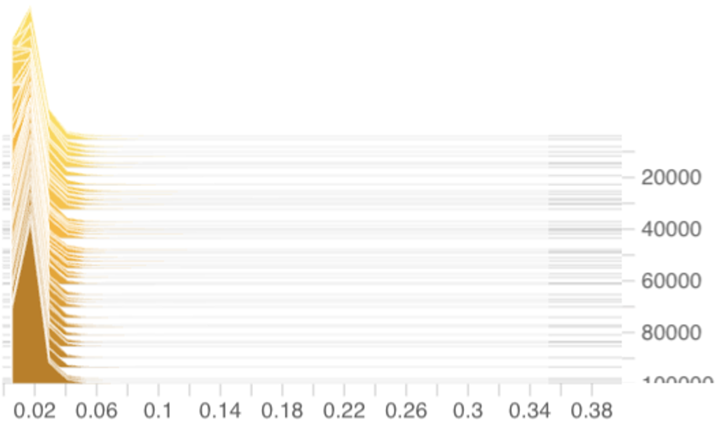
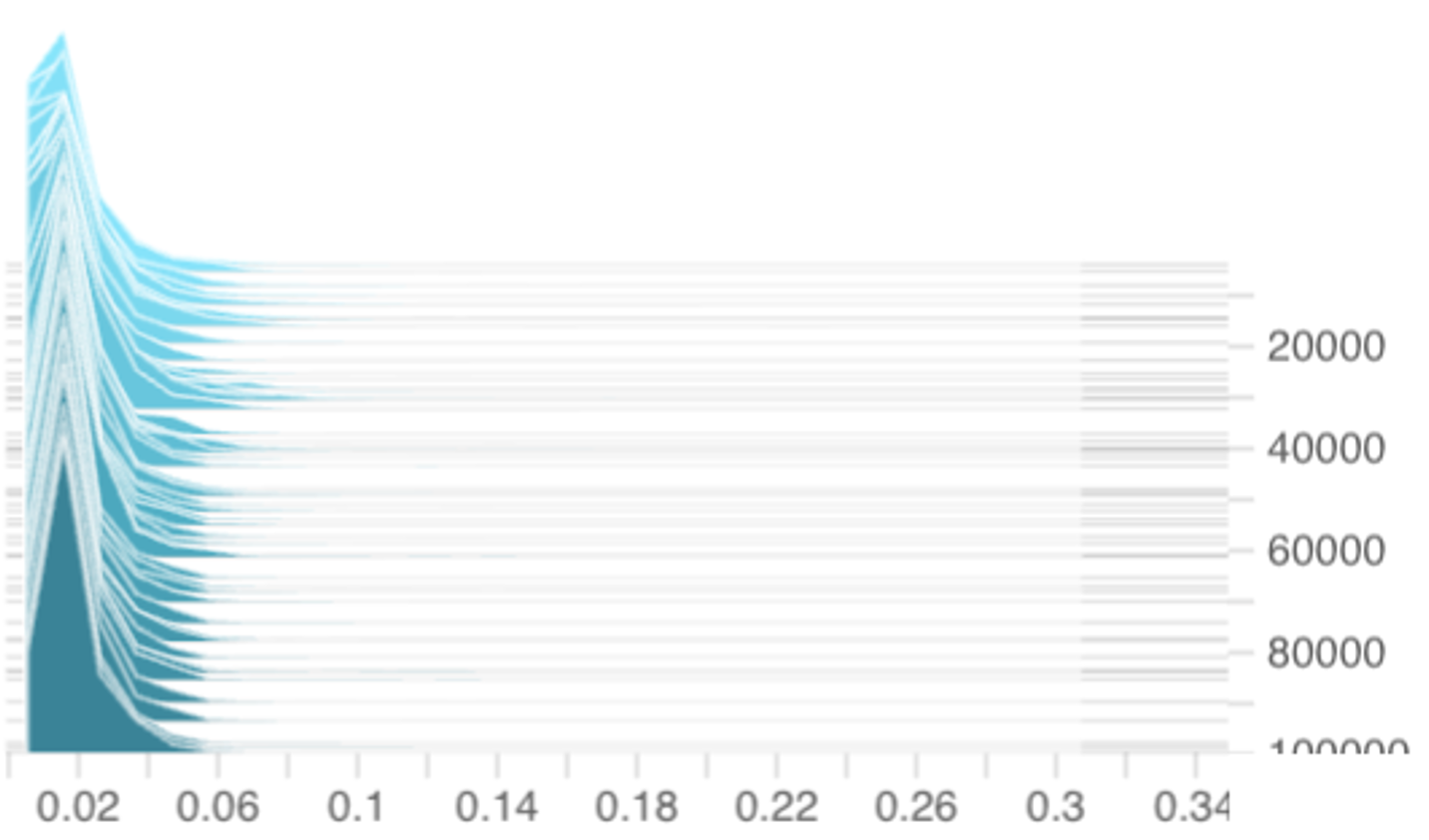
for the i-th token in the n-th iteration are i.i.d across i and n. While this assumption may seem strong, our experiments in Figure 3 from training 1B-parameter DeepSeekMoE models suggest that it is close to reality.

It is easy to check that the loss f (n) is convex. Thus, the expected loss f (p) = E f (n) (p) p is also convex. We first show that the loss gradient g (n) (p) is an unbiased estimator of ∇f (p) with an explicit form expression.

where 1 is the ones-vector, and π(p) ∈ R E is the selection probabilities vector with k-th coordinate

for some generic affinities

Proof. For a given token i, let

Since the distribution of Γ (n),i is independent of i, observe that

To calculate ∇f , we can move the differentiation into the expectation via the dominated convergence theorem: the Γ k have continuous densities so ties occur with probability zero; thus, for almost every realization, the partial derivative ∂ p k m∈TopKInd(Γ+p) (Γ m + p m ) exists and equals 1{k ∈

The desired result follows.

Using Proposition 8, we can compute the variance and second moment of g (n) (p).

Proposition 9. (Variance and 2nd Moment) The variance and second moment of g (n) (p) are given by

Proof. Using Equation (11) and Proposition 8,

E (p) is the vector of expert loads. Let X i (p) ∈ {0, 1} E denote the assignment vector for token i with components as in (12). Then,

Var(X 1k | p) by identical distribution across i

Finally, decomposing the second moment and applying Proposition 8 gives

This completes the proof.

Proposition 9 will be useful later to prove Theorem 13.

In the following Sections 5.4-5.6, we show that the expectation of the Top-K objective is strongly convex with respect to p updates under certain (realistic) assumptions. The strong convexity then allows us to show a logarithmic regret bound in Theorem 13. Without strong convexity, it is routine to verify that the regret bound is at best O( √ N ) without additional assumptions. The next lemma characterizes the second directional derivative of the expected objective.

Proposition 10 (Second Directional Derivative). Let Γ = (Γ 1 , . . . , Γ E ) be a random affinity vector in R E with the properties in Section 5.2. For biases p ∈ R E define

and let φ k and Φ k denote the density and CDF of Γ k , respectively. Then, for any direction δ ∈ R E , its second directional derivative at p is given by the formula

where the symmetric edge weights are

Proof. For some fixed argument γ ∈ [0, 1] E , define the function

is the joint density of Γ. For t ∈ R, define p(t) := p + t δ and F K (t) := F K (p(t)). Since ties occur with probability zero, F K is a.s. differentiable with gradient ∇F K (p) = π(p). Hence, the chain rule gives

We will next compute F ′′ K (0). For each k, using independence and conditioning on

where Φ c j (•) := 1 -Φ j (•) and S represents possible index sets within the top-K components of Γ + p that are also larger than v + p k . For notational convenience, set

Then,

Consider the integrand

For each j, because Φ j is differentiable everywhere on R except (possibly) at 0 or 1, the derivative of the integrand ( 14) with respect to t at t = 0 exists for all but finitely many v ∈ (0, 1). Thus, the integrand ( 14) is differentiable at t = 0 for almost all v ∈ (0, 1).

Next, observe that for each fixed S ⊆ [E] \ {k}, the product in ( 14) has the a.e. derivative

.

This leads to a telescoping cancellation across r in the integrand ( 14). Specifically, for each fixed r < K-1 and ℓ, every index set S r such that |S r | = r corresponds to another index set S ℓ r+1 such that |S ℓ r+1 | = r + 1 and S ℓ r+1 = S r ∪ {ℓ}. It is easy to check that Ξ + Sr,ℓ = Ξ - S ℓ r+1 ,ℓ . So, the sum in ( 14) telescopes over r except at the r = K-1 boundary where Ξ + S K-1 ,ℓ has no corresponding “Ξ - S ℓ K ,ℓ " term to cancel with. Hence, for almost all fixed v ∈ (0, 1),

Next, for any non-zero h ∈ R, it is routine to check that the assumptions in Section 5.2 imply that the integrand of the following is uniformly bounded:

Therefore, by the dominated convergence theorem, we have that π k (p(t)) is differentiable at t = 0, with the derivative being given (after a change of variables) by

Finally, by symmetry,

which is exactly (13).

Observe that the TopKInd decision of the MoE router is invariant to adding the same constant to all coordinates of p. Motivated by this, we define the zero-sum subspace

where Z is the linear subspace orthogonal to the all-ones vector. Thus, we assume the following about ALF-LB for some update direction δ ′ :

Remark 11 (Practicality of Z Assumptions). The assumption (15) is not artificial; it arises naturally from the problem definition:

• Zero-sum gradients. Since k A

(n) k (p)=T K, the components of the gradient (11) sum to zero:

Thus, any update of the form

automatically preserves p (n+1) ∈ Z as long as p (n) ∈ Z. In practice, we initialize with p (0) = 0, so the projection in ( 15) is just the identity mapping.

• Explicit Z-projection with per-coordinate step-sizes. In the more general case where heterogeneous step-sizes ϵ

(n)

k are used across coordinates,

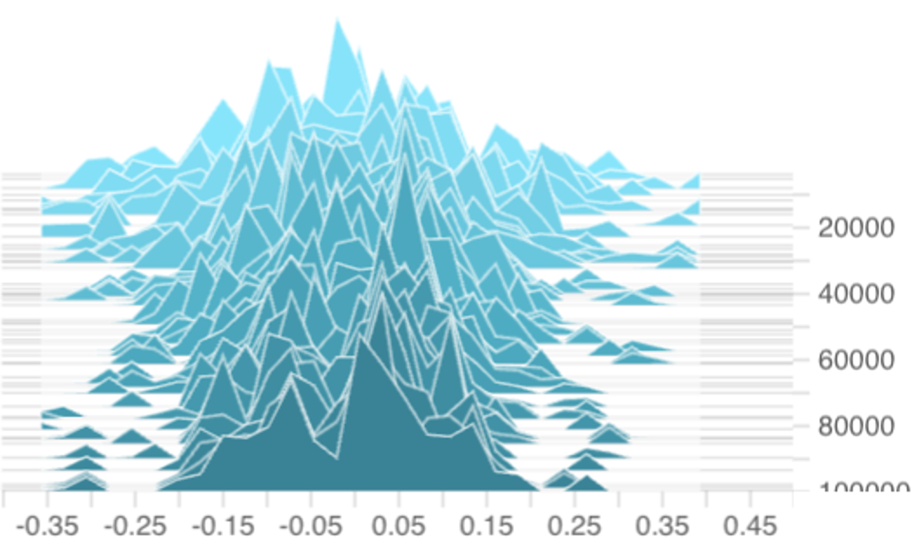
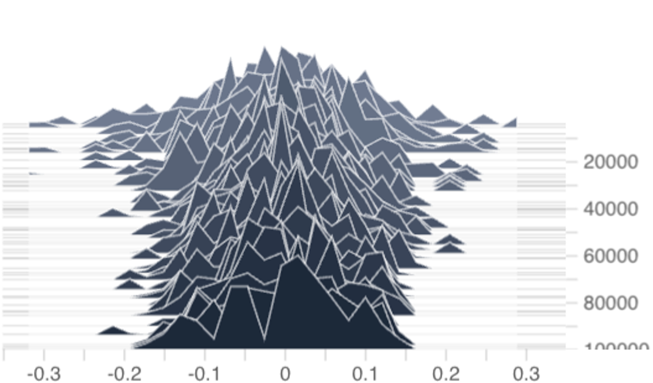
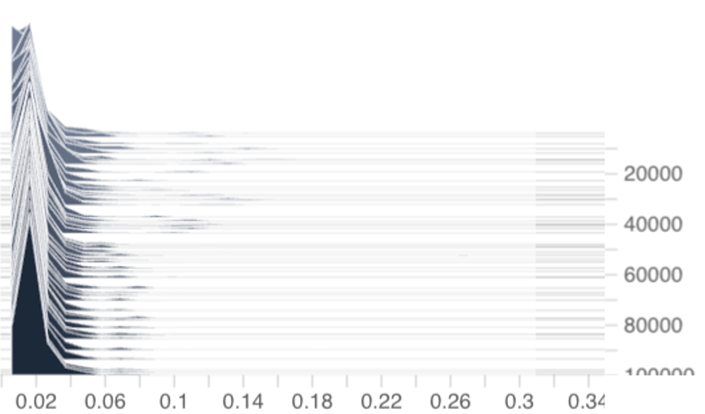
, the updated p (n+1) may not reside in Z. (In fact, the difference between per-coordinate step-sizes and homogeneous step-sizes can be seen in Figure 4 where the per-coordinate ϵ

k | step-size results in a bias distribution that shifts rightward over time while the homogeneous ϵ (n) = u/n and ϵ (n) = u/ √ n step-sizes result in bias distributions that stay centered around zero.) However, in this per-coordinate step-size case, it is well-known that the projection onto Z is equivalent to subtracting the componentwise mean:

which is computationally negligible. Additionally, we will make the technical assumption that diam(p) := max j p j -min j p j ≤ 1 -κ for some constant κ > 0, which we found holds without explicit enforcement in our experiments on 1B-parameter DeepSeekMoE models (Figure 4). Thus, we can realistically assume p ∈ dom κ Z := {p ∈ Z : diam(p) ≤ 1 -κ}.

Next, observe that the component densities of the affinity scores Γ are continuous and strictly positive on (0, 1). Thus, by the continuity of w Hence, by Proposition 10,

The assumption (15) ensures that p (n) ∈ Z for all n. Thus, since Z is a linear subspace,

Since the update direction δ lies in Z,

Combining with property (16), this yields

Recall the expected loss is f (p) = T F K (p) -L k p k and observe the linear term does not affect curvature; thus, for all p, δ ∈ Z with p having diameter at most d, f is µ K -strongly convex with Since f is µ K -strongly convex in Z, p * is necessarily unique.

Define the regret R N := N n=1 f (n) (p (n) ) -f (n) (p * ) . We now give a logarithmic bound on the expected regret E[R N ] with the ALF-LB update p (n+1) ← Proj Z p (n) -ϵ (n) ∇f (n) p (n) .

(18)

While the details are adapted to the specific problem at hand, the proof technique is standard in online convex optimization (see, for example, Hazan (2016, Section 3.3.1)). For clarity, define the following short-hand notations:

Lemma 12 (One-step accounting). Under the assumptions and notations of Section 5.1-5.6, for any ϵ (n) >0, the iteration (18) satisfies

Proof. Since Z is a linear subspace, the projection operator is nonexpansive. Thus, n) , p (n) -p * + ϵ (n) 2 ∇f (n) p (n) 2 .

Taking conditional expectation and using Proposition 8 gives

Since the TopKInd decision is invariant to adding the same constant to all coordinates of p, we can assume without loss of generality that p * ∈ Z. Thus, since Z is a linear subspace, p (n) -p * ∈ Z.

Then, the µ K -strong convexity of f in Z (Section 5.6) gives

Combining the last two expressions, taking total expectation, and rearranging gives

Recall from Section 5.1 that the gradient is ∇f Substituting this bound into (20) yields the desired result.

Theorem 13. (Logarithmic Regret) Consider the update (18) run for N iterations with ϵ (n) = 1/(µ K n). Then,

T,E,K 2µ K (1 + ln N ).

Proof.

Observe that E[R N ] = N n=1 a n . Summing (19) over n = 1, . . . , N gives

The first term on the right-hand side is a telescoping sum which evaluates to

Dropping this non-positive term, we are left with

Invoking the classic N n=1 1 n ≤ 1+ ln N inequality and dividing by 2 yields the desired result.

This is a stylized assumption for the initial analysis in this section only. Later, in Section 5, we will consider the case where the affinity scores are new stochastic realizations from some distribution every iteration.

One notable exception is the BASE layer heuristic invented byLewis et al. (2021) which aims to approximately solve the IP using a truncated auction algorithm modeled afterBertsekas (1992).

We will not include the shared experts within the theoretical framework presented in this paper because the shared experts represent a fixed computational load that does not require dynamic balancing. Additionally, omitting the shared experts from our theoretical formulation leads to cleaner and more concise analyses.

This independence assumption is a stylization: various mechanisms (attention, layer norm, etc.) in earlier layers could create dependencies between token embeddings. However, it gives us a starting point for building a tractable, baseline theory. Furthermore, Figure3demonstrates that the distributions of γ (n) ik remain stable and well-behaved throughout training on DeepSeekMoE-1B models, which indicates that independence is empirically well-founded as an approximating simplification at least at the marginal distribution level.