Content-Aware Texturing for Gaussian Splatting
📝 Original Info
- Title: Content-Aware Texturing for Gaussian Splatting
- ArXiv ID: 2512.02621
- Date: 2025-12-02
- Authors: Panagiotis Papantonakis, Georgios Kopanas, Fredo Durand, George Drettakis
📝 Abstract
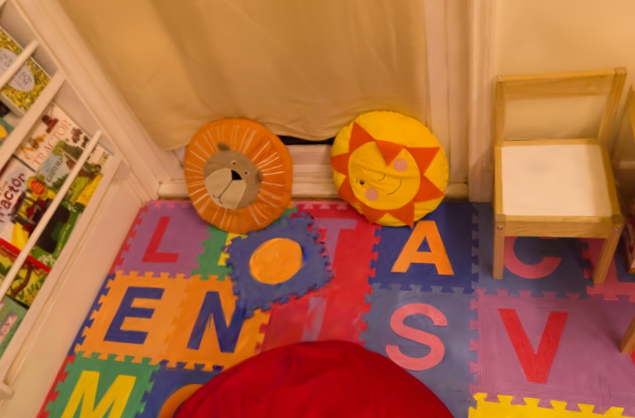
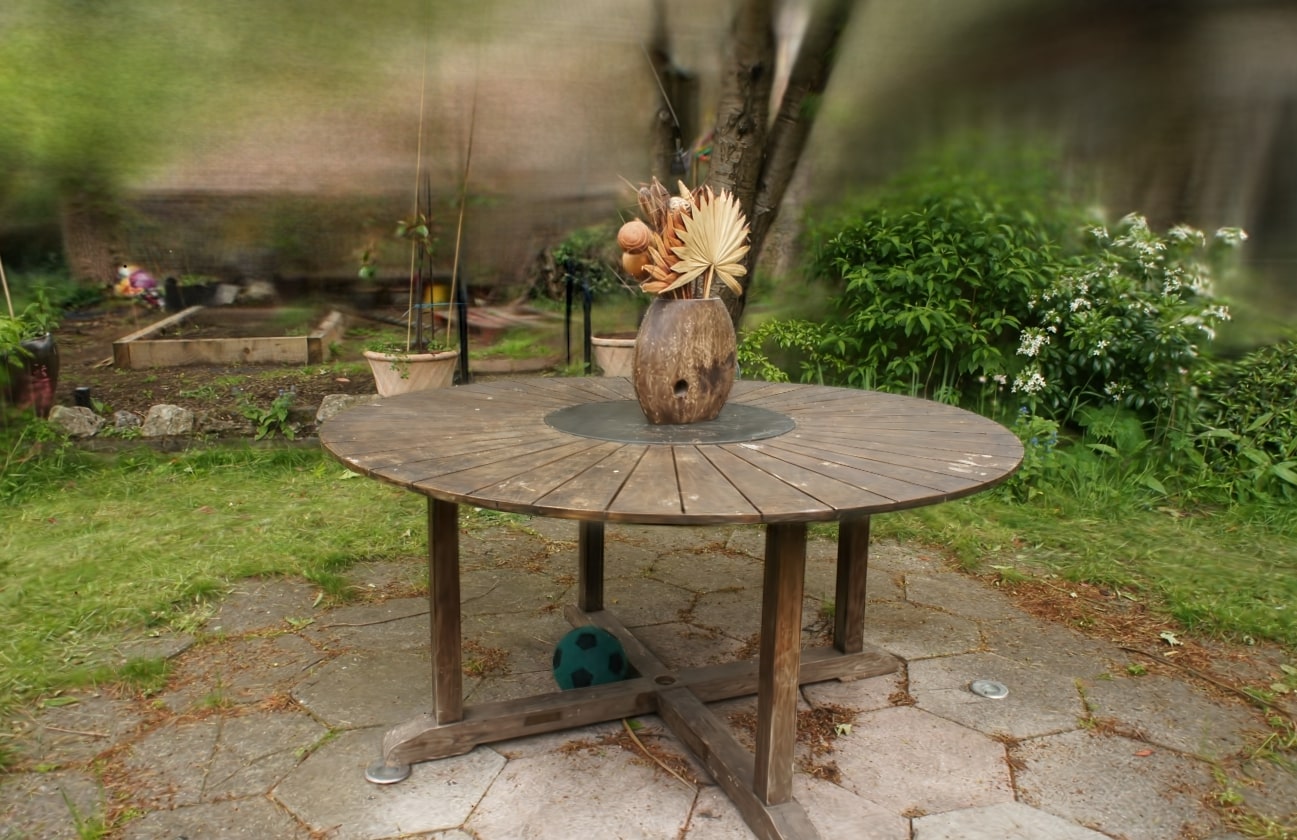
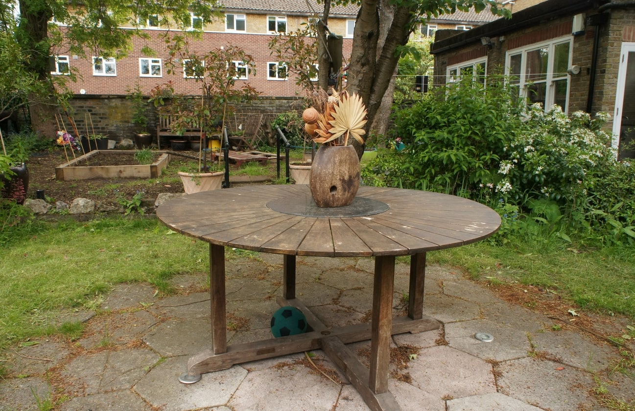
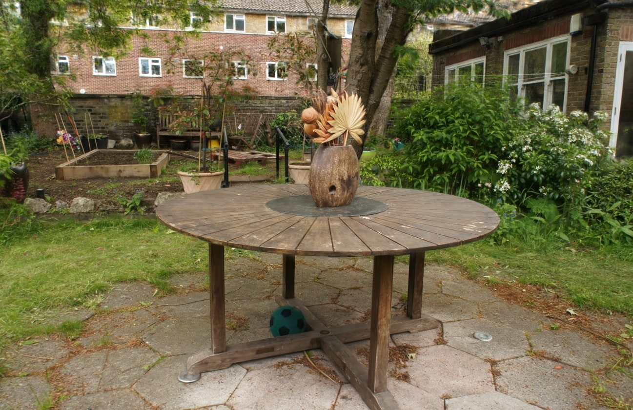
Appearance (c) Fine (d) Coarse (b) Off Texture Figure 1: We propose a content-aware texturing method for 2D Gaussian Splatting. Our textures reconstruct intricate scene detail (a). Gaussian primitives reconstruct the shape of the scene at low frequency of appearance; we show this in (b) where texturing is disabled. Our method is adaptive, allowing different primitives to have different texel sizes, depending on scene content. On the right hand panel we display primitives with progressively higher texel-to-pixel ratio. In regions with high frequency appearance, texels have size close that of pixels (e.g., the table cover (c)). For the low-frequency walls however (d), the ratio is high, with each texel representing a large number of input image pixels.📄 Full Content
In recent and concurrent work [SMAB25; RCB25; CTP25; XCW24] a number of methods introduce textured Gaussian primitives, providing a spatially varying color. Most of these methods use planar 2D Gaussians to match the dimensionality of traditional textures. Each primitive carries several parameters (position, rotation, scale, opacity and spherical harmonics (SH)), while textures are 2D arrays of RGB(A) texels. The fundamental challenge of such approaches is how to allocate model capacity across the scene and between the number of texels and the number of primitives used. Previous and concurrent solutions either deal with the issue by imposing a fixed texture resolution per primitive [SMAB25; XCW24; CTP25], or propose heuristic approaches, that are far from ideal [RCB25]. This leaves open the question of how to share resources in a more principled manner.
To answer this question, we propose a content-aware texturing solution for 2D Gaussian primitives that uses the appearance complexity as observed from the input images of the scene to make informed decisions on how parameter resources are distributed. We do this by first introducing a textured Gaussian primitive representation in which texel size is fixed in world space. This makes the appearance texture of each primitive independent of its size, and therefore unaffected by the growing or shrinking that it undergoes during optimization. This representation separates the parameters of geometry and appearance, allowing us to refine them independently with appropriate allocation of memory capacity. More specifically, we introduce a method to increase and decrease the texel size as optimization evolves, by analyzing the frequency content that primitive textures can represent and determining the corresponding error. We pair that with a resolution-aware method to control the overall number of primitives, striking a balance between texture size and number of primitives. Our solution interacts closely with the optimization, using the downscale/upscale mechanism to reduce the error in appearance, while our control of the number of primitives handles geometric error by spawning additional Gaussians to capture geometric detail.
In summary, we propose three contributions:
• A texture representation for 2D Gaussians that defines texels with a fixed world space size, supporting visual reconstruction independent of the shape of the primitives. • A progressive algorithm that adaptively determines texel size and allows for content-aware fitting of the scene. • A resolution-based solution to control the number of primitives, adjusted to the textured representation.
Our experiments show that our method provides a good balance between visual quality and the number of parameters used for the representation, comparing favorably to other textured Gaussian primitives solutions proposed in recent and concurrent work.
Texture Mapping was introduced in the early days of CG [Cat74] and is widely used to effectively map detailed appearance infor-mation onto a simpler geometric representation, such as triangles.
Textures are stored as 2D image arrays with a mapping function between the 3D surface and 2D texture coordinates. Computing this 2D surface parameterization is a well-studied and difficult problem [HLS07; LKK18; SGV24]. Intrinsic 2D parameterizations pose challenges even in traditional graphics pippelines [YLT19] because they introduce difficulties in content creation and produce visual artifacts in rendering. In the context of optimization for inverse problems -such as novel view synthesis -intrinsic parameterizations are also challenging since the geometry is not known in advance [SGV24]. An alternative, non-parametric way to store localized information on the surface is by attaching it on the primitives themselves, i.e., attaching colors to the vertices of a mesh, requiring a very fine mesh subdivision to represent details. Mesh Colors [YKH10;MSY20] extend this idea by using more color samples along the edges and the faces of the triangles. This significantly improves the representational capacity of non-parametric appearance textures. While non-parametric appearance models are limited in many ways, they have significant advantages in the context of optimization since they overcome the need to jointly solve for texture parameterization and the surface. Our representation is also a non-parametric texture representation for Gaussian Splatting. Gaussian Splatting [KKLD23] has emerged as an alternative, point-based approach to NeRFs by replacing the volumetric field with a collection of semi-transparent ellipsoidal primitives. This technique achieves excellent quality and real-time rendering even at high resolutions. Several methods built on top of 3DGS to provide anti-aliasing [YCH24], by changing the appearance model but are constrained by the 1-to-1 relationship between color samples and primitives [YGS24; MST25].
2D Gaussian Splatting [HYC*24] flattens one of the dimensions of the ellipsoids to create planar discs or surfels to align bet-ter with surfaces. Surfels are parametrized by the set of parameters A = {µ, σ, q, o, SH}, where µ ∈ R 3 is the primitive’s center, σ ∈ R + 2 are the scales of the primal axes of the surfel, q ∈ R 4 is a quaternion that represents the rotation R, o is the opacity and SH are the spherical harmonics coefficients used to get the viewdependent colour c. The normal vector n of the surfel is the third column of the rotation matrix R.
With this formulation, the intersection point between a ray r = r 0 + td and a primitive can be computed as:
We also build on 2D Gaussian Splatting for our method.
The initial primitive-based representations were not as compact as NeRFs, but a number of recent results allow competitive compression strategies [BKL24]. Several recent methods build on traditional CG solutions, demonstrating that disentangling appearance from geometry can achieve significant improvements in terms of storage and memory costs. Texture-GS [XHL24] combines deferred shading and a per-pixel UV coordinate to fetch appearance from a texture. This assumes that the objects can be represented by a sphere imposing topological constraints. Our results demonstrate that non-parametric texture mapping is a convenient and flexible way to recover texture during the optimization.
Recent and concurrent work [SMAB25; CTP25; XCW24; RCB*25] have used textures to represent fine visual details.
[RCB25] and [CTP25] use converged 2DGS and 3DGS point clouds, respectively, as a starting point of their method, and then proceed to add and optimize texture parameters. Several methods [SMAB25; CTP25; XCW24] use a fixed texture resolution for each primitive that is a hyperparameter of the method. GS-Tex [RCB25] distributes a texel budget over the primitives proportional to their size, resulting in different resolutions for differentsized primitives. All these methods define their textures in the Gaussian canonical space, with the textures undergoing the same transformations as the primitive, which leads to texture stretching and shrinking. SuperGaussians [XCW24] also experiment with representing the texture with a small Neural Network. In our approach, we explore a different and more robust design that allows for texture maps to dynamically adjust to the captured content. Along with two strategies that control the size of the texels and the number of primitives that are designed specifically for our representation, we are able to reconstruct scenes without the need for a pretrained model.
We first define a new representation for appearance of the Gaussian primitives that allows for content-aware texturing. We then show how to adapt the texturing process to scene content, by taking into account the different screen-space frequencies that need to be represented using textures. This is achieved in a progressive manner that is compatible with the optimization process. Finally, we propose a resolution-based primitive management method that splits primitives allowing the geometry and appearance of the scene to be approximated as required.
In contrast to the original 2D Gaussian Splatting approach [HYC*24] (see Sec. 2.2 and Eq. 1), we express the intersection between a camera ray and a primitive in different coordinate systems, denoted by a superscript. This is done, as some coordinate systems make some operations easier. Specifically:
• p w = p is the intersection point in world space, • p w0 = p wµ is in world space, centered on the primitive, • p l = R -1 p w0 is in the local, axis-aligned coordinate system of the primitive. Since the last component of this point is 0, we consider that p l ∈ R 2 • p c = S -1 p l , where S = diag(σ) is in the local, normalised coordinate system of the primitive. This last coordinate system can be considered as the “canonical” space of the Gaussian primitive. The use of these spaces is purely to facilitate some operations. For instance, Eq. 1 is evaluated in the camera view space, where r 0 is on top of the origin, while anything that involves querying the texture map is better done in a coordinate frame local to the respective primitive.
The color of a ray r is computed by alpha blending:
where w i (p i ) is the contribution of the Gaussian, G(x) is the evaluation of the Gaussian function that defines the falloff G(x) = e -1 2 (x T x) , and T i is transmittance.
We augment each 2D Gaussian primitive with a texture map T . The texture map adds a spatially varying offset c T to the original spherical harmonic color representation. The texture colors vary only spatially and have no directional dependency. This representation is compact and models only the diffuse properties of the surface, akin to albedo multiplied by irradiance. As a result, the color of each primitive is now also dependent on the intersection point between the ray emanating from the pixel and the 2D primitive:
where u are the coordinates in UV space at which the ray intersects primitive i with a direction vector d, and SH are the spherical harmonics. We need to carefully design the texture coordinate calculation that transforms the intersection point into local, normalized primitive space p c to UV coordinates. As we discuss below, it is especially important to consider how this mapping changes when the primitive parameters are updated during optimization.
A simple mapping from the canonical space to UV texture space fixes the relative texture coordinates on the primitive such that the texture will stretch and deform with scaling and rotation of the primitive:
where s i is the extent of the texture in units of standard deviations of the Gaussian primitive, and Tres is the texture resolution. When the extent of the texture is smaller than the primitive, some type of padding needs to be applied. Difference between two mappings for a primitive having learned a particular texture. Top row: a naive approach distorts the appearance after the primitive undergoes scaling. Bottom row: in our approach, as texel size is fixed in world space, scaling the primitive only reveals more part of the underlying texture, preserving existing content.
Recall that primitives change size and shape during the optimization process. As a result, with such a texture mapping, the appearance parameters of the texture are coupled with the parameters that control the shape of the primitive. During optimization, small changes in the scale of the Gaussians result in changes of all the values of the texture. This can induce local minima in the optimization process that are visible as texture stretching, see Fig. 2 (top).
Instead, we define a content-aware representation in which textures are adapted to scene content. Our goal is to have textures that can faithfully represent the frequency of image details at the highest resolution present in the input images. To do this, we fix the texel size with respect to the optimization process such that no optimizable parameters change it. We achieve this with a small modification to Eq. 5:
where k i is the texel size and T offset is an offset to center the texture map. In constrast to Eq. 5, the intersection point p l and hence the texel size k i are defined in world space, with the same units as the primitive’s scales σ.
This mapping implies that the textures do not have a fixed texture resolution. On the contrary, as the primitives grow or shrink, more or less texture resolution is needed to cover their surface. This is demonstrated in Fig. 2 (bottom). We modified our optimization routines to allocate and de-allocate texture resolution dynamically.
Since the number of texels can grow quadratically, we risk running out of resources if every primitive has a texture. Our goal is to maintain an expressive representation while carefully managing resources. To achieve this, we enforce two properties on our representation: First, the projected sampling frequency of the texture needs to be bounded by the image sampling frequency of the closest camera. This means that the projected texel size should never be smaller than the smallest input pixel that can see it. Second, texel sizes should adapt to scene content, i.e., smaller texel sizes should be allocated for high frequency image content.
The first goal can be achieved using a conservative choice to determine minimum texel size as the pixel size back-projected in world space from the input training view closest to the primitive’s center k p min , similarly to [PKK*24]. Regarding the second goal, optimal texel sizes cannot be determined at initialization since pritimives change size and rotate dynamically during optimization. We need a way to adapt to the freqency content of the scene progressively. To do this, we next introduce an adaptive strategy to determine texel size during optimization, where we downscale and upscale texture by adapting to the scene content. We complement this approach with a resolutionaware primitive management method that add primitives to represent geometric -rather than appearance -error. We describe these two components in the following sections.
Our goal is to adapt textures to the frequency content of the input images. We also need to achieve this in a progressive manner that fits well with the optimization process. We define a texel sizeto-pixel size ratio t 2 p r , which we manipulate during optimization using downscaling and upscaling operations.
We define the texel size k based on the minimum pixel size k p min , with t 2 p r as follows:
We use this parameter to assign a low t 2 pr to primitives in regions with fine details. As a result, such primitives will have more texels for a given primitive size. Similarly, primitives that lie in areas with low-frequency appearance will have a higher ratio, giving them relatively fewer texels. To provide a lower bound of 1 and facilitate texture rescaling operations, t 2 pr can only take values that are powers of two.
To this end, we propose two strategies to increase and decrease t 2 pr leading to a downscale and an upscale of the texture map respectively. Note that texel size and texture resolution are linked, but not the same. In the operations below, when texel size changes, texture resolution will change but only because the primitive size is unchanged.
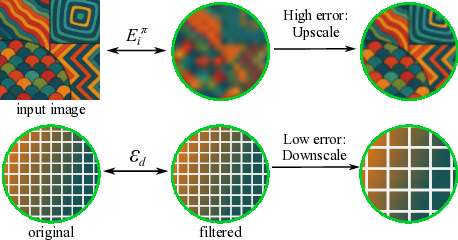
Increase of texel size-to-pixel size ratio -Downscaling: Our goal is to find texture maps that represent low frequency details and decrease their texel size accordingly. We do this by applying a lowpass filter on textures and then comparing them to the originals.
The error E d is weighted by the Gaussian falloff of the primitive, leading to the following equation:
If this error is less than a threshold τ ds , we assume that the texture map can be reconstructed with good-enough fidelity by the downscaled version. Hence, we double t 2 p r , which reduces the total number of texture parameters by 4. This reduces the resolution of texture, since the world-space size of the texels has grown. The size of the primitive is however unchanged.
Decrease of texel size-to-pixel size ratio -Upscaling: In regions where the texel size of the primitives involved is too large to capture the fine, underlying details, we expect our images to be blurry, and thus induce large error. To identify these regions, we estimate primitive error using the approach presented in [RPK24]. Specifically, for a primitive i, a ray r, a camera view π and corresponding RGB error image Eπ, we compute the per primitive error for a single view:
where P i are all the pixels covered by the primitive. Here we assume that we have one ray per pixel, emanating from its center.
Differently from [RPK24], instead of taking the maximum error over views, we perform a weighted sum, with the weight being the total contribution of a primitive in that image.
where Π is the set of all input views. This choice assigns an error value to each primitive that is proportional to their contribution to the rendered image.
We choose the top 10% of primitives with the highest error, and upscale their textures by a factor of 4, by halving t 2 pr. With smaller sized texels, these primitives can better fit to the scene content, reducing their error.
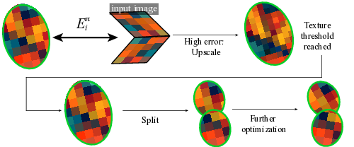
Progressive texel size adaptation. The calculation of the per primitive error E i and the application of upscale/downscale process happens regularly during optimization. Texel size adapts to scene content during this process, getting bigger for primitives that lie in low-frequency regions, and smaller for primitives that exhibit large error, as shown in Fig. 1
There are two main sources of error: appearance and geometry. For the first case, our upscaling approach reduces error as the optimization progresses. However, for the case of geometry that is not well represented, an additional step is required. To address this and complete our content-aware method, we next introduce resolutionaware splitting.
In Gaussian splatting methods where each primitive contains one color sample, densification -i.e., adding new primitives through cloning and splitting -plays an essential role in improving the reconstruction of the scene. This results in a local increase in both the geometric (position, scale, rotation) and appearance parameters (SH, opacity) that are treated together since they are tied to a single Gaussian primitive. However, this is not always ideal, since there are cases where the geometry is low frequency and has been approximated well, but we are missing texture detail, or conversely, cases where the color information is low frequency, but the underlying surface is not correctly represented. The latter case can appears as holes, “softened” edges or elongated primitives in places where they are not required. The primitive has been upscaled to a resolution greater than τtr in both axes. Our splitting approach creates four new primitives, each with half the scale and texture resolution in both axes.
Our separation of geometric and appearance parameters provides an additional degree of freedom, allowing us to independently decide whether to increase the number of parameters linked to geometry, i.e., increasing the number of primitives or to appearance, i.e., increasing texture resolution.
Given that we do not have a supervision signal explicitly for geometry, we attempt to first match the appearance, using the upscaling approach described above. If the error is still high despite upscaling, we interpret the remaining error as geometric. In these cases, we can add more primitives, locally increasing the geometric degrees of freedom. We found that densification strategies that were based on cloning either partially [KKLD23] or entirely in the case of 3DGS-MCMC [KRS*24], are incompatible with our representation. This is because the superimposition of multiple textured primitives makes convergence difficult and requires an excessive number of parameters. As a result our primitive management is based on splitting, which fits well with our method. We describe this next.
Similar to the approach for upscaling, we take the top 10% of primitives with the highest error, and check which of these exceed a threshold τtr for texture resolution. The primitive is replaced by two new primitives, each displaced by ±1 standard deviation of the Gaussian. This process is performed separately for each axis; the new primitives have half the scale (size) in each corresponding axis, as a result, half the texture resolution, G(1) times the opacity, where G is the Gaussian. The texture map of the newly added primitives is created by sampling the original point at the respective locations. Fig. 4 illustrates the splitting process for a primitive that happens to have a texture resolution greater than τtr in both axes. A flowchart of how upscaling and splitting interact is shown in Fig. 5. Alg. 1 displays in high level how the two methods are integrated in code. Table 1: We compare our method against 2DGS* trained with no geometric regularisations, BBSplat and GSTex, with default settings. We show standard quality metrics (PSNR, SSIM, L-PIPS), total number of primitives, texels and parameters. Our method achieves competitive results while using significantly fewer, highly expressive primitives. We also include 3DGS-MCMC for completeness; please note that 3DGSbased methods achieve better NVS but worse geometry quality compared to all approaches based on 2DGS (see discussion Sec. 5.1). Figure 5: The primitive has high error, and successive upscalings result in a texture resolution above threshold. In this case, the error is geometric rather than due to appearance. Our algorithm performs a split, and further optimization will match the geometry.
As in [KKLD23], we train our model using the weighted sum of the per-pixel L 1 and the structural similarity losses, between the ground truth and the rendered images:
with λ SSIM = 0.2.
We observed that textures could finish converging to highfrequency settings, even though alpha-blending would create a smooth result. This prevented them from being downscaled, leading to high parameter usage. To resolve this, we apply a sparsity regularization on the texel values, pushing them towards zero,
We constrain the texel values in the [-1, 1] range, using a sigmoid activation, scaled and shifted accordingly:
where σ(x) is the sigmoid function and c ′Ti are the unactivated texture features. Intuitively, this parametrization coupled with the sparsity loss forces the view-dependent color SH(d) to learn the base color of the surface, while the texels operate as offsets to model high-frequency details. An example of this is illustrated in Fig. 1(left).
Finally, as in [PKK24; KRS24], we incentivize lowcontribution primitives to effectively disappear by applying an opacity regularization term:
Taking both training objectives and regularizations into consideration, the total loss is formed as:
(15)
We have implemented our method using the 3DGS codebase, introducing 2D primitives as in 2DGS. Unlike 2DGS, we do not use the R 2 → R 2 transformation to find the intersection point using three non-parallel planes. Instead, we use Eq. 1 directly in camera space. We did not observe any instability issues. Since our method requires per-ray querying of texture maps, both the forward and backward passes incur additional overhead, that is not compensated by the smaller number of primitives rendered. In general, compared to 2DGS, training time is 1.5-2 times longer, and rendering is 25% slower.
As the texture grids can have different resolutions, we created custom “jagged” tensor data structure to be used for their storage. The texture resolution for each primitive gets (de-)allocated dynamically, so that it covers the extent of the primitive, that is ±3 We provide renderings from one scene per dataset for every method, trained with default settings. Our method is able to reconstruct high frequency details on images, even while using fewer parameters compared to the other methods.
standard deviations. This dynamic memory management happens every 100 iterations. A hard limit of 256 texture resolution is enforced to avoid using too much memory. When a primitive grows outside of its allocated texture grid, either because memory has not been allocated yet or it has surpassed the hard limit, zero-padding is used. Since we are storing an offset, zero-padding reduces to the DC color.
We observed that limiting the t 2 pr to be greater or equal to 2 did not have a detrimental effect on the visual quality, as subtexel scaled details can be retrieved thanks to alpha blending and the overlap of our primitives. We thus allow upscaling to happen only for primitives with a t 2 pr greater or equal to 2.
Storage and Memory Considerations. The size of our representation is tied to the number of parameters used, with each parameter saved as a 4-byte float, as in previous Gaussian Splatting implementations. However, most Gaussian Splatting compression techniques (see [BKL*24]) are applicable to our approach either directly or with minor modifications. For our newly introduced texture maps, our choice to use a sigmoid activation to limit the effective range of the texel values allows for a very efficient application of K-means clustering compression. Please see Tab. 5 for complete statistics.
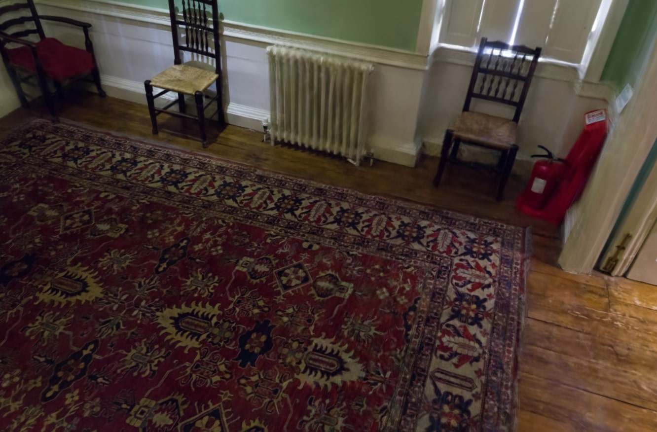
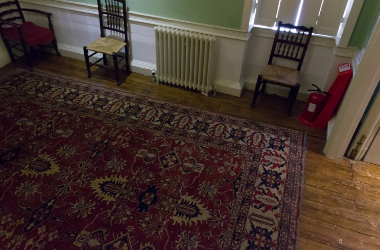
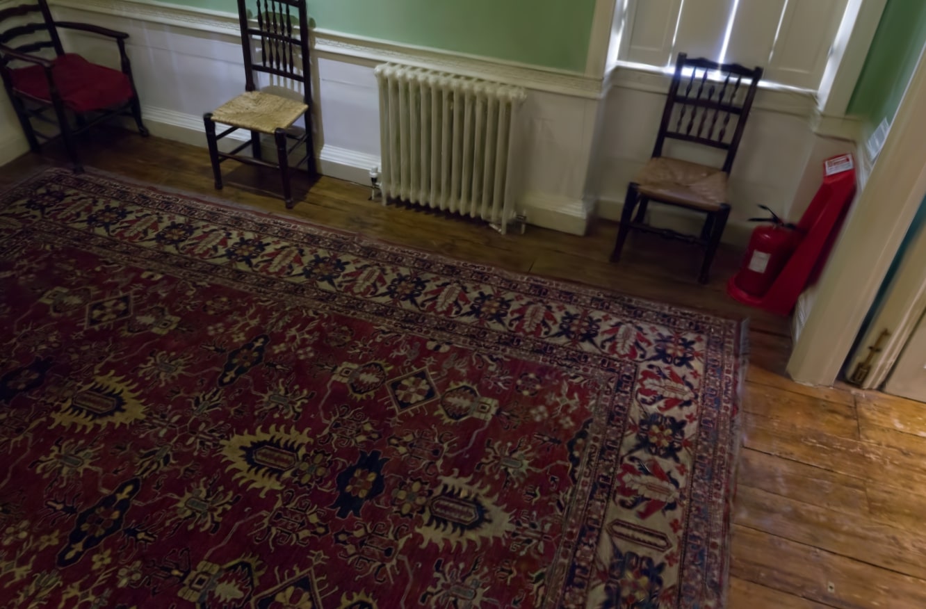
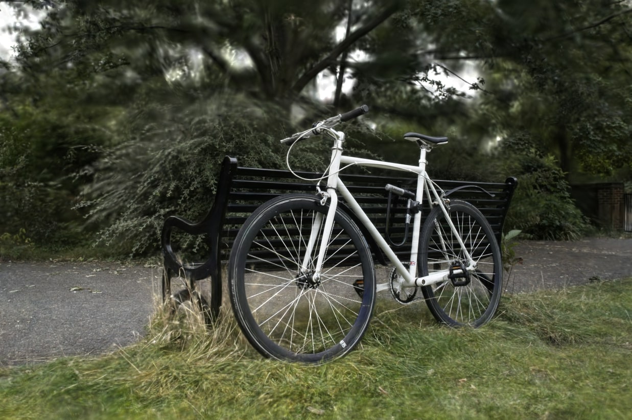
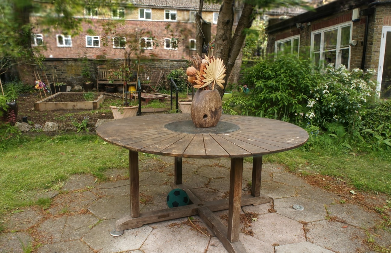
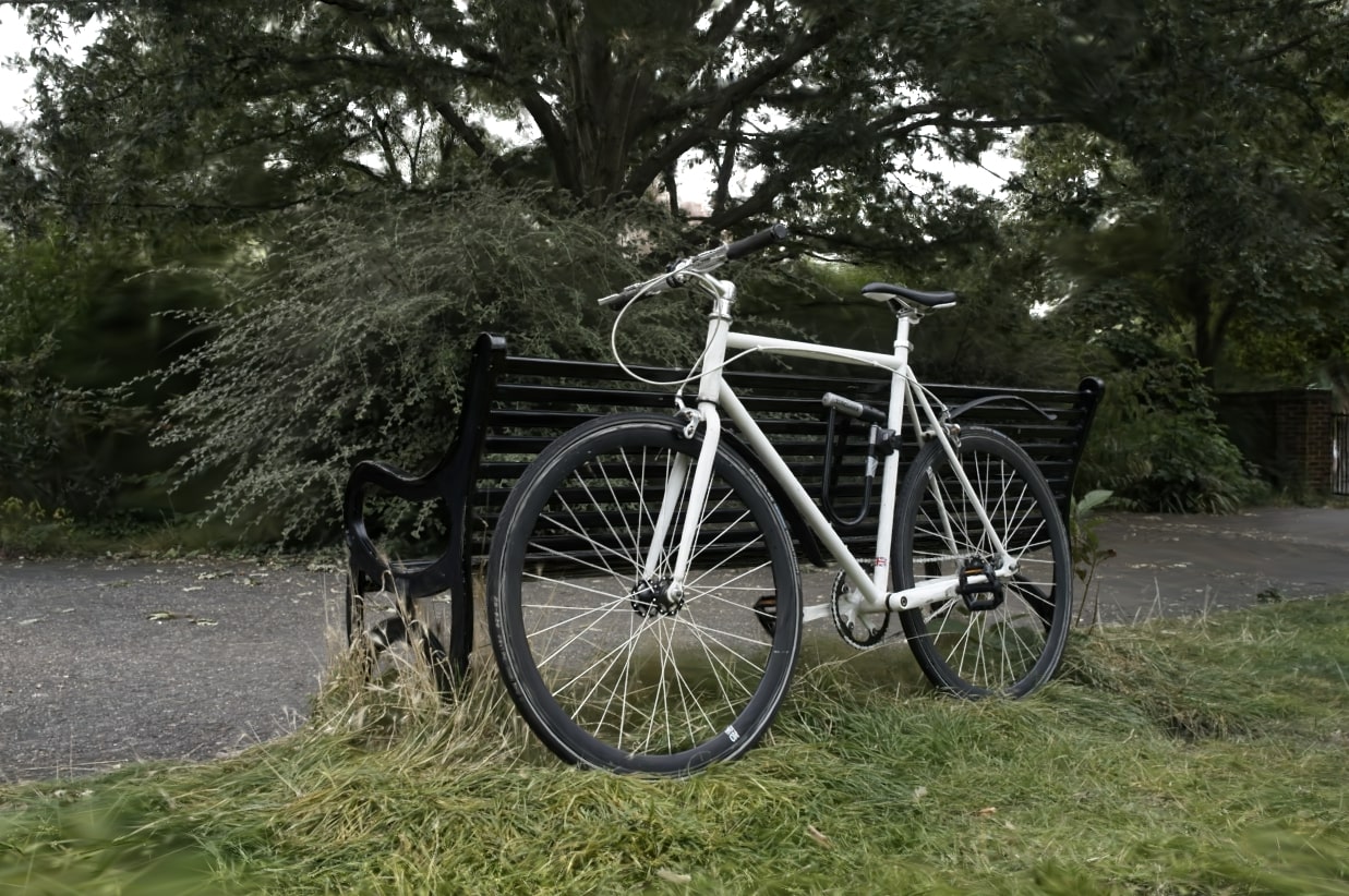
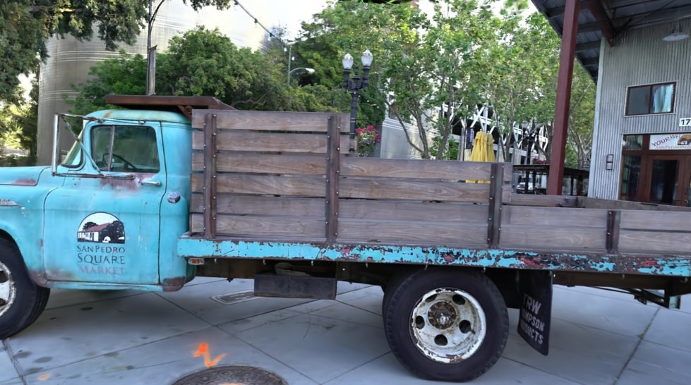
We test our method on 13 indoor and outdoor scenes from three different standard datasets. We evaluate on all scenes of Mip-NeRF 360 [BMV22], two scenes from Tanks & Temples [KPZK17], as well as two scenes from Deep Blending [HPP18]. Fig. 6 shows that our method faithfully reconstructs the input images.
We compare our method against 2DGS [HYC24] as a baseline, and two 2DGS texturing methods, namely (unpublished) BB-Splat [SMAB25] and GStex [RCB25], for which the code was available at the time of submission. Directly comparing to 3DGSbased models is not straightforward and might lead to misleading conclusions, since these models have different properties and consistently perform better for NVS but worse in geometry reconstruction, compared to 2DGS-based solutions [HYC24]. For the same reason, and because the code was not available at the time of submission, we do not compare against [CTP25], which is a 3DGS-based method with textured primitives. This model uses a pretrained 3DGS-MCMC model as initialization, similar to GStex, and includes RGBA textures, similar to BBSplat. We thus expect it to suffer from the disadvantages of both these two models (see discussion of the second experiment). We ran these methods on all scenes using our machines to ensure fair comparison. For 2DGS, the normal consistency and depth distortion regularization terms were disabled, as they are designed to enhance the geometric reconstruction but often result in lower novel view synthesis (NVS) quality.
Qualitative Evaluation. In Figure 6, we show visual results for the different models. We show test views (i.e., not used for training) from one scene of each dataset. Our method succeeds in reconstructing high-frequency details with high fidelity, even with fewer parameters. Similarly, Figure 7 displays visual results from the second experiment, which highlight that other texturing methods struggle when constrained to the same parameter budget as ours. GSTex uses a point cloud that is not trained with textured primitives in mind and a static heuristic distribution of texels, which causes it to not reconstruct well large parts of the scene. BBSplat succeeds in geometrically reconstructing the scene, but exhibits texture stretch- ing, which appears as blurriness. This is due to the choice of mapping between intersection points and UV coordinates.
Quantitative Evaluation. For our quantitative comparisons, we present results for three error metrics, SSIM, PSNR, and LPIPS [ZIE*18], that are typically used to evaluate NVS. Additionally, we report the number of primitives and texels used, which provides a precise measure of the resources required for each method and demonstrates whether and how much textures contribute to the scene reconstruction. Finally, since the models’ capacity is directly tied to the number of parameters used, we include the relevant column so that we can make fair comparisons and draw meaningful conclusions.
The formula for the number of parameters differs slightly among the models. For 2DGS, GSTex each primitive has 58 parameters (3 for position, 2 for scale, 4 for rotation, 1 for opacity, 48 for color), while for BBSplat this number is 57, as it lacks opacity. In our method, in addition to the parameters of 2DGS, we include one additional per primitive for the texel size, pushing the number to 59 parameters. Regarding the parameters coming from texels, GSTex and our method have 3 per texel, while BBSplat has one additional, corresponding to the alpha channel.
In Table 1, we compare methods trained with default settings. In most cases, our approach achieves competitive or superior quality across all three metrics, while requiring a lower number of trainable parameters. Focusing on the composition of these parameters, our converged models have significantly fewer, but more expressive primitives than the baseline as illustrated in Fig. 1 (left). This highlights the ability of our model to account for the difference in complexity between geometry and appearance. In contrast, GSTex uses a pretrained 2DGS point cloud and has a fixed budget of tex-els, distributed at initialization time; this results in limited usage of texture. This is in part because it starts with a converged set of primitives from 2DGS that is not well adapted to a solution with texture. On the contrary, we optimize both primitives and textures from scratch. Moreover, while our primitive count is close to BBSplat’s, the total number of parameters used is significantly lower than theirs. This can be attributed to our content-aware texel size determination, which dynamically allocates model capacity to regions according to their needs, as opposed to the fixed texel to primitive ratio that BBSplat imposes.
To emphasize the importance of our content-aware texturing approach, we next compare the other texturing methods by fixing both the primitive and texel budgets to ours. In GSTex this is feasible, because it allows the distribution of a given texel budget over a pretrained 2DGS point cloud. We first trained 2DGS with the specified primitive budget and then gave the texel budget as input to GSTex. However, in BBSplat, controlling both the primitive and texel budgets is not possible, as the method imposes a fixed ratio between the two, determined by the texture resolution (16x16). Therefore, we calculated the number of primitives that would result in the same number of trainable parameters. Table 2, reports these results under these fixed parameters. Note that BBSplat uses a skybox to model background and distant objects in outdoor scenes, which was not taken into consideration when calculating the number of primitives. This accounts for the slight discrepancy in the number of parameters. Both the other methods observe a noticeable to significant drop in performance. This is possibly due to the fact that model capacity is not distributed efficiently both across primitives and across parts of the scene. In this setup, our method performs consistently better on average than previous solutions.
As a third experiment, we run our method with a low, fixed primitive budget, by skipping the splitting procedure whenever the model exceeds it. The adaptive texel size strategies were left unchanged. Table 3 shows the results. As expected, the performance gets better with an increasing primitive count, as the use of primitives with a fixed gaussian falloff prevents faithfully reconstructing sharp edges with sparser point clouds. However, we note that the number of texels does not grow proportionally to the number of primitives or even diminishes, in the case of Tanks & Temples. This is a direct result of our choice of texture coordinate mapping function and the adaptive texel size determination strategy. Our separation of geometric and appearance parameters allows our models to automatically achieve a balance between the two that is appropriate for the scene.
Our method presents a good balance of resources used for textured Gaussian Splatting, allowing a smooth variation between number of primitives and number of texels used to represent a scene. However, like all other methods that build on 2DGS, we do not achieve the quality of 3DGS. Using 3D primitives with texture raises interesting questions about how to represent texture: should one use a 2D texture on a plane, or rather a voxel or hash-grid in 3D ? While Textured-GS [CTP*25] proposes a first solution using the former approach, the analysis presented in the paper is insufficient to determine how well the choices made perform compared to our solution.
We do not have any special treatment for anti-aliasing. For NVS, the user can only navigate freely within -or at least close -to the convex hull of the input cameras. Since we choose a t 2 pr value that is at least 2, aliasing will rarely by occuring in this range of viewpoints. Nonetheless, a complete solution for anti-aliasing would be an interesting avenue of future work.
We did not investigate the use of dedicated GPU hardware capabilities for texture. Given that our implementation of textured Gaussian Splatting uses a custom CUDA renderer, it is unclear how beneficial this would actually be. However, for the case, e.g., of We-bGL renderers [Kwo], this may be a much more interesting direction that could allow accelerated rendering, especially in the case of low-end hardware.
We have presented a new representation for textured 2D Gaussian Splatting, that is driven by scene content. By adaptively choosing texel size to fit the content of the scene, and carefully balancing resources used with our resolution-aware spltting approach, we provide a versatile method that allows users to choose between more primitives or more texture while preserving image quality. Our method provides an additional point in the design space of primitive-based NVS algorithms, building on the long tradition of texture mapping in CG rendering.
© 2025 The Author(s). Proceedings published by Eurographics -The European Association for Computer Graphics.
📸 Image Gallery