Atomic Diffusion Models for Small Molecule Structure Elucidation from NMR Spectra

The molecules that sustain life come in several forms: large biopolymers such as DNA, RNA, and proteins described by our genetic code, and small molecules, which form complex metabolic pathways and influence all aspects of biology. A category of small molecules, known as secondary metabolites or natural products, describes those that are secreted into the environment where they serve myriad functions, such as signaling and chemical warfare. Because of these roles, natural products have delivered more than half of the FDA-approved small-molecule agents, including the majority of antibiotics and antitumor drugs in current clinical use, such as penicillin, taxol, and other blockbuster drugs such as lovastatin and semaglutide [48,14,68,58]. To identify an unknown molecule's structure, 1D NMR spectroscopy measures peaks corresponding to each proton ( 1 H) or carbon ( 13 C) atom (middle). The resulting chemical shifts (x-axis locations), peak intensities, and J-coupling (splitting patterns) encode information on chemical groups and connectivities, from which the molecular structure can be deduced (right).

The functions of small molecules are intrinsically linked to their molecular structures, which govern their chemical and biological reactivity. Very recently, deep learning methods have revolutionized the prediction of a protein’s 3D structure from its amino acid sequence encoded in the genome [30,2]. Small molecules, by contrast, are neither directly genetically encoded nor repeating polymers. Structure elucidation therefore relies on de novo experimental methods for every new molecule, making the discovery of cellular metabolites, essential molecules, antibiotics, and other therapeutics a slow and tedious process [8,48,18].

Nuclear Magnetic Resonance (NMR) spectroscopy is a cornerstone technique for small molecule structure elucidation. This experimental method provides information regarding the connectivity and local environment of, typically, each proton ( 1 H) and carbon ( 13 C) in a molecule, thus allowing the structure of a molecule to be deduced. However, the inverse problem of inferring the chemical structure from these spectral measurements is a challenging puzzle, which largely proceeds manually and requires significant time and expertise, even with computational assistance [8]. Consequently, automating molecular structure elucidation directly from raw 1D NMR spectra would significantly accelerate progress in chemistry, biomedicine, and natural product drug discovery [56,47,77,42,17].

With the rise of deep learning approaches applied to molecules, diffusion generative models [20,59,32] have emerged as powerful tools for tasks such as small molecule generation [21,46,69,40], ligand-protein docking [10,57], and protein structure prediction [2,73] and design [25,70,15]. While early approaches emphasize 3D geometric symmetries via equivariant networks, recent trends suggest that non-equivariant transformers scale more effectively with model and data size and better capture 3D structures with data augmentation [69,2].

In this work, we tackle the challenging task of NMR structure elucidation for complex natural products. We introduce CHEFNMR (CHemical Elucidation From NMR), an end-to-end diffusion model designed to infer an unknown molecule’s structure from its 1D NMR spectra and chemical formula. CHEFNMR processes NMR spectra using a hybrid transformer with a convolutional tokenizer designed to capture multiscale spectral features, which are then used to condition a Diffusion Transformer [49] for 3D atomic structure generation. To scale to the complex chemical groups found in natural products, we curate SpectraNP, a large-scale dataset of synthetic 1D NMR spectra for 111,181 complex natural products (up to 274 atoms), significantly expanding the chemical complexity of prior datasets (≤101 atoms) [22,4]. We compare CHEFNMR against chemical language model-based and graph-based formulations and demonstrate state-of-the-art accuracy across multiple synthetic and experimental benchmarks.

NMR spectroscopy is a widely used analytical technique in chemistry for determining the structures of small molecules and biomolecules. A typical one-dimensional (1D) NMR experiment measures the response of all spin-active nuclei of a given type, for example hydrogen ( 1 H) or isotopic carbon ( 13 C), to radiofrequency pulses in a strong magnetic field. The resulting spectrum consists of peaks from chemically distinct nuclei, where peak positions (i.e., chemical shifts), intensities, and fine splitting patterns (i.e., J-coupling) reflect local chemical environments and connectivities of the nuclei.

Formally, let the observed spectrum be a real-valued signal S(δ) : R → R, where δ denotes the chemical shift (in parts per million, ppm) along the x-axis. The signal can be modeled as a sum over N resonance peaks corresponding to each spin-active nucleus:

where A i is the intensity (amplitude) of the i-th peak, δ i is the chemical shift (peak center), and γ i is the linewidth (related to relaxation) of the peak. L(δ; δ i , γ i ) is the normalized Lorentzian line shape:

and ϵ(δ) models additive noise (e.g., Gaussian white noise or baseline drift). J-coupling refers to the splitting of the signal for a given nucleus into a sum of multiple peaks when nearby atoms interact:

where M i is the number of split components for the i-th nucleus, and δ ik encodes the shifted peak positions. J-coupling occurs when other spin-active nuclei are within 2-4 edges in the molecular graph, and the signal splits into M i = m + 1 components assuming m interacting nuclei. See Figure 1 for an example.

Together, these features encode rich information about the types of chemical groups present and their connectivities, enabling chemists to deduce the underlying molecular structure. For example, certain chemical groups produce peaks that appear at an established range (e.g., aromatic ring-protons are detected at 6.5-8 ppm), whose exact location depends on the amount of chemical shielding from nearby atoms in a given molecule. These patterns, in addition to experimental noise due to the instrument, impurities, and solvent effects, make the inverse problem of deducing structure an extremely challenging task. NMR structure elucidation thus typically relies on additional information from 2D NMR experiments, prior information on the substructures present, or chemical formula from high-resolution mass spectrometry [7] combined with isotopic abundance and distribution patterns. In this work, we use the chemical formula as an auxiliary input, as it is typically the most readily obtainable among common priors and effectively constrains the space of candidate molecular structures for complex natural products.

In this section, we present CHEFNMR, an end-to-end diffusion model for molecular structure elucidation from 1D NMR spectra and chemical formula. Our approach consists of two key components: NMR-ConvFormer for spectral embedding (Section 3.1) and a conditional diffusion model for 3D atomic coordinate generation (Section 3.2).

In CHEFNMR, we represent molecule-spectrum pairs as (A, X, S), where A ∈ {0, 1} N ×datom denotes the one-hot encoding of atom types for a molecule with N atoms and d atom possible atom types, X ∈ R N ×3 represents the 3D atomic coordinates, and S = (s H , s C ) contains the NMR spectra, specifically the 1 H spectrum s H ∈ R dH and the 13 C spectrum s C ∈ R dC . Our objective is to generate the 3D coordinates X conditioned on the atom types A (i.e., chemical formula) and the spectra S by sampling from the conditional probability distribution p(X|A, S).

Position & Type Encoding Layer Norm & Linear

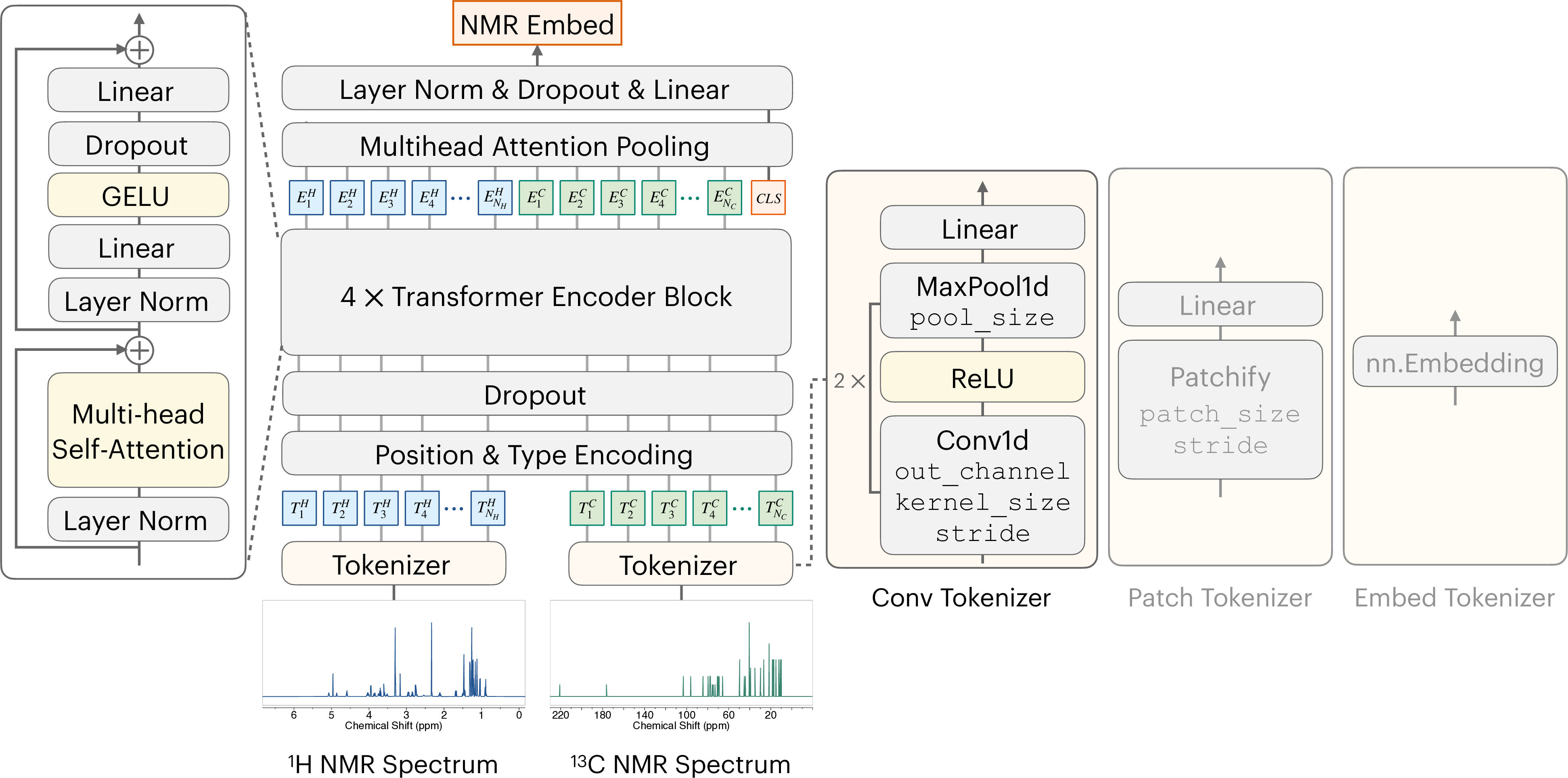
To effectively condition the generative process on the NMR spectra S, we propose NMR-ConvFormer, an encoder designed to capture both local spectral features and global correlations within and between the 1 H and 13 C spectra, as shown in Figure 2(a). Unlike prior methods that rely solely on 1D convolutions [22,45] or transformers with simple patching [67,63], NMR-ConvFormer uses a hybrid approach, combining a convolutional tokenizer for local feature extraction and a transformer encoder for modeling complex intra-and inter-spectral dependencies.

Convolutional Tokenizer. Each input spectrum ( 1 H and 13 C) is processed independently by a convolutional tokenizer comprising two 1D convolutional layers with ReLU and max-pooling, similar to [22]. This reduces sequence length while increasing channel dimensions, summarizing local patterns like peak intensity and splitting. The output is linearly projected to dimension D encoder , yielding token sequences of shape (T, D encoder ).

Transformer Encoder. The token sequence, augmented with positional and type embeddings, is processed by a standard transformer encoder comprising multi-head self-attention and feed-forward networks with pre-layer norm and residuals. Self-attention captures patterns within each NMR spectrum and across different spectra, such as related peaks in a 1 H spectrum or matching signals from the same chemical group in both 1 H and 13 C spectra.

Multihead Attention Pooling (MAP). We use MAP [37,79] to obtain a fixed-size spectral embedding. A learnable [CLS] token prepended to the encoder output sequence aggregates information via a final self-attention layer. The resulting [CLS] token state, after layer normalization and linear projection, serves as the conditioning vector z S ∈ R Dhidden for the diffusion model. Dropout is applied at multiple stages to mitigate overfitting. See Appendix D.2 for detailed hyperparameter settings.

Training Objective. We adapt the EDM diffusion framework to conditional 3D molecular generation [32]. The model D θ is trained to predict clean 3D coordinates X 0 from noisy inputs X σ = X 0 + n, where n ∼ N (0, σ 2 I) and the noise level σ is sampled from a pre-defined distribution p(σ). Given X σ , σ, atom types A, and spectral embedding z S , the model minimizes:

where X0 = D θ (X σ ; σ, A, z S ) are the predicted coordinates.

The MSE loss, L MSE = ∥ X0 -X 0 ∥ 2 2 , enforces global structure alignment. To ensure local geometric accuracy (e.g., bond lengths), crucial for chemical validity and often poorly captured by MSE alone, we add a smooth Local Distance Difference Test (LDDT) loss [43], adapted from AlphaFold3 [2]. The LDDT score is computed over all distinct atom pairs (i, j):

Here, dij = ∥ xixj ∥ 2 and d ij = ∥x 0,i -x 0,j ∥ 2 are the predicted and true distances, respectively. Thresholds t k ∈ {0.5, 1.0, 2.0, 4.0 Å} specify allowable deviations between predicted and true distances when evaluating prediction accuracy. The smooth LDDT loss is L smooth_lddt = 1 -LDDT, encourages local geometric fidelity by penalizing pairwise deviations. The combined loss promotes both global alignment and local chemical validity.

For each molecule, we generate k ground-truth conformers.

During training, we randomly sample one conformer X 0 and apply a random rigid transformation (translation and rotation) following [2,29,40]. This augmentation encourages D θ to learn SE(3)invariant representations and mitigate overfitting, significantly improving performance.

Diffusion Transformer (DiT) Architecture. The network D θ is a DiT [49] shown in Figure 2(b). Input atom tokens are formed by concatenating noisy coordinates X σ and atom types A, followed by an MLP projection. The noise level σ is embedded using frequency encoding and an MLP. This noise embedding is added to the spectral embedding z S to form the conditioning vector, which is integrated into the DiT blocks via adaptive layer normalization (adaLN-Zero) [49].

Conditional Dropout and Classifier-Free Guidance. To improve robustness and flexibility in conditioning on different NMR spectra, we adopt classifier-free guidance (CFG) [19]. During training, the 1 H NMR spectrum is dropped with probability p H = 0.1, the 13 C NMR spectrum is dropped with p C = 0.1, and both are dropped simultaneously with p both = 0.1. At inference, conditional and unconditional predictions are combined via

where ω ≥ 0 controls guidance scale. This enables generation conditioned on either or both spectra, improving versatility and performance. See Appendix A and D.2 for full training and sampling algorithms and hyperparameter settings.

NMR Spectra Prediction. The forward task of predicting a given molecule’s NMR spectra is relatively established, facilitating data analysis and enabling the generation of simulated datasets for structure elucidation of simple compounds via database retrieval. These spectra prediction methods range from precise, computationally intensive quantum-chemical simulations to more recent exploratory ML approaches [6,28,13,35,31,16,39,44]. Following established dataset curation practices [22,4], we create our SpectraNP dataset using the commercial software MestReNova [44], which combines closed-source ML and chemoinformatics algorithms.

NMR Structure Elucidation. Structure elucidation from NMR spectroscopy is a challenging inverse problem, due to the complexity of spectra data and the vast size of chemical space [60,17]. Traditional computer-aided systems, while historically employed and useful, often suffer from computational inefficiencies [8]. Recent ML methods have tackled this challenge, but most simplify the problem by predicting molecular substructures instead of full molecules [38,36,5,64,76,33], or by leveraging richer inputs, such as additional experimental data beyond NMR [54,12,50,55,11,9,63,53] and database retrieval [78,62,33]. In contrast, our method directly tackles the de novo elucidation of molecular structures using only raw 1D NMR spectra and chemical formulae.

De Novo Structure Elucidation from 1D NMR Spectra. Recent work developing machine learning methods for de novo structure elucidation from 1D NMR spectra focuses on structurally simple molecules, leveraging either chemical language models or graph-based models. Chemical language models [80,22,3,4] generate SMILES strings [71], a sequence-based molecular representation. For example, Hu et al. [22] use a multitask transformer pre-trained on 3.1M substructure-molecule pairs and fine-tuned on 143k NMR spectra from SpectraBase [26], achieving 69.6% top-15 accuracy for molecules under 59 atoms. Alberts et al. [3,4] employ transformers to predict SMILES from text-based 1D NMR peak lists and chemical formulas, reporting 89.98% top-10 accuracy on the USPTO dataset [41] for molecules under 101 atoms. Graph-based models iteratively construct molecular graphs with GNNs, using methods like Markov decision processes or Monte Carlo tree search [27,23,61]. However, these methods do not handle molecules with more than 64 atoms or large rings (>8 atoms), likely due to the limited availability of large-scale spectral datasets and the high computational cost of search-based algorithms for complex molecules. To the best of our knowledge, CHEFNMR is the first method based on 3D atomic diffusion models for NMR structure elucidation that scales to complex natural products.

3D Molecular Diffusion Models. Diffusion models have emerged as powerful tools for 3D molecular generation. E(3)-equivariant GNNs [74,21,75,46] enforce geometric constraints, but non-equivariant transformers are increasingly favored for their scalability and performance in small molecule generation [69,40,29] and protein structure prediction [2,15] involving hundreds of thousands of atoms.

Inspired by these recent trends, we apply a scalable DiT [49] to generate 3D atomic structures from NMR spectra, exploiting their scalability and expressivity by creating a large synthetic NMR spectra dataset of natural products. Synthetic Datasets. We evaluate models on two public benchmarks, SpectraBase [22] and USPTO [4], and our self-curated SpectraNP dataset. SpectraBase contains simple molecules [22,26], while USPTO features a broader range of molecules in chemical reactions [41]. SpectraNP combines data from NPAtlas [52], a database of small molecules from bacteria and fungi, with a subset of NP-MRD [72] including various natural products.

Experimental Datasets. To evaluate the ability of models trained on synthetic data to generalize to experimental data, we curate two experimental datasets. Following [4], we include the SpecTeach dataset [65], which contains 238 simple molecules for spectroscopy education. We also include NMRShiftDB2 [34], a larger-scale dataset of 13 C NMR spectra in various solvents, following [61,28]. These experimental datasets include impurities, solvents, and baseline noise (See Figure 5), enabling robustness testing for experimental variations.

Data Structure and Preprocessing. Each data entry is a tuple (SMILES, 1 H NMR spectrum, 13 C NMR spectrum, atom features). SMILES strings are canonicalized with stereochemistry removed, and synthetic spectra are simulated using MestreNova [44]. Atom features include atom types A and 3D conformations X, generated using RDKit’s ETKDGv3 algorithm [1] given the SMILES string.

To preprocess datasets, any duplicate SMILES are first removed. 1 H and 13 C spectra are interpolated to 10,000-dimensional vectors following [22,4], and normalized by their highest peak intensity, except for SpectraBase [22] and experimental datasets, where 13 C spectra are binned into 80 binary vectors. To validate 3D conformers, SMILES strings are reconstructed from atom types and 3D coordinates using RDKit’s DetermineBonds function [1], and molecules failing reconstruction are discarded. See Appendix C for dataset curation details.

Baselines. We compare CHEFNMR against two existing chemical language models and introduce a graph-based model to assess the impact of molecular representations on the structure elucidation task.

The chemical language models are: (1) Hu et al. [22] propose a two-stage multitask transformer for predicting SMILES from 1D NMR spectra. Their method pre-defines 957 substructures and pre-trains a substructure-to-SMILES model on 3.1M molecules, and then fine-tunes a multitask transformer on 143k NMR spectra from SpectraBase. We retrain their substructure-to-SMILES model on the same 3.1M dataset and fine-tune it on each synthetic benchmark. (2) Alberts et al. [4] develop a transformer to predict stereochemical SMILES from text-based 1D NMR peak lists and chemical formulae. Due to unavailable inference code and differences in input (peak lists vs. raw spectra) and output (stereo vs. non-stereo SMILES), we report their published results on USPTO and SpecTeach.

To test an alternative graph-based representation, we also propose NMR-DiGress, a model integrating the discrete graph diffusion model DiGress [66] Metrics. We evaluate models using: (1) Top-k matching accuracy, which checks whether the ground truth SMILES string is exactly matched by any of the top-k predicted molecules. For nonlanguage models, we reconstruct canonical, non-stereo SMILES from the predicted molecular graph (atom types and generated bond matrix) or 3D structure (atom types and generated 3D coordinates) using RDKit [1]. (2) Top-k maximum Tanimoto similarity, which evaluates structural similarity between the ground truth and the most similar molecule in the top-k predictions, using the Tanimoto similarity of Morgan fingerprints (length 2048, radius 2) [1].

This section presents the quantitative and qualitative results across benchmarks. Section 6.1 shows CHEFNMR’s state-of-the-art performance on synthetic datasets, and Section 6.2 demonstrates robust zero-shot generalization on experimental datasets. Section 6.3 presents ablation studies on the contributions of the diffusion training process and the NMR-ConvFormer spectra embedder.

Table 2 summarizes the performance on synthetic 1 H and 13 C NMR spectra. CHEFNMR significantly surpasses all baselines in matching accuracy and maximum Tanimoto similarity across datasets. The Performance scales up with both model and dataset size. CHEFNMR-S outperforms baselines by large margins across all datasets, and CHEFNMR-L further improves accuracy. Larger datasets also yield better results, with the highest performance observed on USPTO (745k data), followed by SpectraBase (141k data) and SpectraNP (111k data). This suggests expanding SpectraNP could further enhance performance in elucidating complex natural products.

Figure 3 provides qualitative examples of CHEFNMR’s performance on SpectraNP. CHEFNMR accurately predicts diverse and complex natural product structures in its top-1 predictions (Figure 3(a)). We additionally show incorrect predictions (Figure 3

Figure 4 reports the zero-shot performance on experimental 1 H and 13 C NMR spectra. CHEFNMR achieves 56% top-1 accuracy on SpecTeach and 21% on NMRShiftDB2, significantly outperforming Hu et al. [22] and NMR-DiGress, which generalize poorly to both experimental benchmarks. Figure 5 shows that CHEFNMR can generate the correct structures in its top-1 predictions despite substantial experimental variations, such as solvent effect and impurities.

We perform extensive ablation studies to assess the contributions of key components in diffusion training and the NMR-ConvFormer on the SpectraBase dataset. Each row in

In this work, we address the challenge of determining structures for complex natural products directly from raw 1D NMR spectra and chemical formulas. We introduce CHEFNMR, an end-to-end diffusion model that combines a hybrid convolutional transformer for spectral encoding with a Diffusion Transformer for 3D molecular structure generation. To encompass the chemical diversity present in natural products, we curate SpectraNP, a large-scale dataset of synthetic 1D NMR spectra for natural products. Our approach achieves state-of-the-art accuracy on synthetic and experimental benchmarks, with ablation studies validating the importance of key design components.

Several limitations highlight promising directions for future work. Expanding the training set to include experimental spectra and more natural products could further improve model performance.

Additional information, such as 2D NMR spectra, could be incorporated to resolve stereochemistry. Furthermore, adding a confidence module could help chemists better assess the reliability of predicted structures. Overall, automating NMR-based structure elucidation has the potential to significantly accelerate molecular discovery. Careful validation and responsible deployment will be essential to ensure safe and impactful use in real-world applications.

In this section, we provide full training and sampling algorithms for the conditional 3D atomic diffusion model described in Section 3.2 of the main paper.

Training Procedure. The complete training procedure is outlined in Algorithm 1. The smooth LDDT loss is detailed in Algorithm 2, adapted from AlphaFold3 [2]. Unlike the original, which computes the smooth LDDT loss within a certain radius for proteins [2], we compute it of all atom pairs for small molecules, as small molecules are more compact in 3D space than proteins.

Algorithm 1 Diffusion Training. 1: procedure SMOOTHLDDTLOSS(predicted coordinates X0, ground-truth coordinates X0, thresholds t = {0.5, 1.0, 2.0, 4.0})

LDDT ← mean i̸ =j (ϵij) ▷ Mean score, excluding self-pairs 7:

Lsmooth_lddt ← 1 -LDDT ▷ Smooth LDDT loss 8:

return Lsmooth_lddt 9: end procedure Preconditioning. To stabilize training across different noise levels, we precondition the denoising network D θ following EDM [32]:

where F θ is the core neural network performing the actual computation. The scaling functions c skip , c out , c in , c noise , and the loss weight λ(σ) are defined as EDM [32]:

Here, σ data represents the standard deviation of atom coordinates in the dataset (see Appendix Table 7).

Conditional Dropout and Classifier-Free Guidance. To improve robustness and flexibility in conditioning on NMR spectra, we adopt classifier-free guidance (CFG) [19]. During training, the 1 H NMR spectrum is replaced with zeros with probability p H = 0.1, the 13 C NMR spectrum is dropped with p C = 0.1, and both are dropped simultaneously with p both = 0.1 (see Algorithm 1). At inference, conditional and unconditional predictions are combined via

where ω ≥ 0 controls guidance scale. This enables generation conditioned on either or both spectra, improving versatility and performance. In this paper, we set ω ∈ {1, 1.5, 2} depending on datasets.

Algorithm 3 Diffusion Sampling using Stochastic Heun’s 2 nd order Method.

1: procedure SAMPLEDIFFUSION(D ω θ (Xσ; σ, A, zS ), atom type A, NMR spectra embedding zS , noise level schedule σ i∈{0,…,N } , γ0 = 0.8, γmin = 1.0, ω guidance scale) 2:

sample X0 ∼ N 0, σ 2 0 I 3:

for i ∈ {0, . . . , N -1} do 4: γ = γ0 if σi > γmin else 0 5:

σi ← σi + γσi ▷ Temporarily increase noise level σi 6:

sample ϵi ∼ N 0, I 7:

Xi ← Xi + σ2 i -σ 2 i ϵi ▷ Add new noise to move from σi to σi 8:

di ← Xi -D ω θ ( Xi; σi, A, zS ) /σi ▷ Evaluate dX/dσ at σi 9:

Xi+1 ← Xi + (σi+1 -σi)di ▷ Take Euler step from σi to σi+1 10:

if σi+1 ̸ = 0 then 11:

▷ Apply 2 nd order correction 12:

Xi+1 ← Xi + (σi+1 -σi)

end for 15:

return XN 16: end procedure Sampling Procedure. The reverse diffusion process begins with X 0 ∼ N (0, σ 2 max I) and iteratively denoises to obtain X N . This process is governed by the stochastic differential equation (SDE) [32]:

where ∇ X log p X; σ|A, z S = D ω θ (X σ ; σ, A, z S ) -X /σ 2 is the conditional score function [24], σ is the noise level, and dw is the Wiener process. The term β(σ) determines the rate at which existing noise is replaced by new noise.

During inference, the noise level schedule σ i∈{0,…,N } is defined as EDM [32]:

where σ max = 80, σ min = 0.0004, ρ = 7, and N = 50 is the number of diffusion steps. The sampling process is performed by solving the SDE using the stochastic Heun’s 2 nd method [32], as outlined in Algorithm 3.

As introduced in Section 5.2 of the main paper, NMR-DiGress is a graph-based baseline model integrating the discrete graph diffusion model DiGress [66] with our NMR-ConvFormer for molecular structure elucidation from 1D NMR spectra and the chemical formula. In this section, we provide a detailed description of the training and sampling procedures of NMR-DiGress.

In Training Procedure. The training procedure of NMR-DiGress is adapted from DiGress [66]. Noise is added to each bond independently via discrete Markov chains, and a neural network is trained to reverse this process to generate bond matrices. Specifically, to add noise to a graph, we define a discrete Markov process {E t } T t=0 starting from the bond matrix E 0 = E:

where Q t is the transition matrix from step t -1 to t. From the properties of the Markov chain, the distribution of E t given E is:

where Qt = Q 1 Q 2 …Q t . Following DiGress, we use the noise schedule:

where ᾱt = cos (0.5π (t/T + s) / (1 + s))

2 , βt = 1 -ᾱt , T = 500 is the number of diffusion steps, and s is a small hyperparameter. Here, m is the marginal distribution of bond types in the training dataset and m ⊤ is the transpose of m. This choice of noise schedule ensures that each bond in E T is converged to the prior noisy distribution (i.e., the marginal distribution of bond types m).

To predict the original bond matrix E from the noisy graph G t = (A, E t ), we train a neural network

, where z G is extra features derived from G t in DiGress and z S is the NMR spectra embedding from NMR-ConvFormer. We use the same graph transformer architecture as in DiGress for ϕ θ [66]. The complete training algorithm is shown in Algorithm 4.

Sampling Procedure. We extend DiGress [66] by conditioning on atom types A and spectra embeddings z S . Each bond in E T is independently sampled from the marginal distribution m to form the noisy graph G T = (A, E T ). For each timestep t, we compute extra features z G = f (G t , t), predict bond probabilities pE = ϕ θ (G t , z G , z S ), and derive the posterior for each bond e ij :

where e can be chosed from d bond bond types. Then each bond in G t-1 is independently sampled according to this posterior. After T steps, the denoised molecular graph G 0 is generated. The complete algorithm is given in Algorithm 5.

In this section, we provide details on the dataset curation process, including the data structure, preprocessing pipeline, and a summary of the statistics for each dataset.

Each data entry is represented as a tuple (SMILES, 1 H NMR spectrum, 13 C NMR spectrum, atom features). The SMILES string is a sequence of characters representing a molecule [71]. Each SMILES string is canonicalized, with stereochemistry such as chiral centers and double bond configurations removed. Only molecules containing the elements C, H, O, N, S, P, F, Cl, Br, and I are retained. Duplicate entries are removed to ensure one unique SMILES per molecule.

The NMR spectra are stored as vectors, and details of the preprocessing steps are provided in Appendix C.2. Atom features include atom types A and 3 ground-truth conformers X, which are generated using RDKit’s ETKDGv3 algorithm [1] from the SMILES string. To validate the generated 3D conformations, SMILES strings are reconstructed from the atom types and 3D coordinates using RDKit’s DetermineBonds function [1]. Molecules that fail reconstruction are discarded. Explicit hydrogens are included to ensure accurate SMILES reconstruction, as required by DetermineBonds.

Synthetic Spectra Simulation. Synthetic spectra are generated from SMILES using MestreNova [44], with deuterated chloroform (CDCl 3 ) as the solvent. Default simulation settings are applied: 1 H spectra (-2 ppm to 12 ppm, 32k points, 500.12 Hz frequency, 0.75 Hz line width) and 13 C spectra (-20 ppm to 230 ppm, 128k points, 125.03 MHz frequency, 1.5 Hz line width, proton decoupled).

Experimental Spectra Collection. SpecTeach [65] experimental raw spectra are in .mnova file format, with default NMR processing steps preserved, including group delay correction, apodization in the time domain, and phase and baseline corrections in the frequency domain if exist.

NMRShiftDB2 [34] has 13 C NMR spectra chemical shift lists.

Spectra Preprocessing. To standardize spectra from different datasets, which vary in chemical shift ranges, resolutions, and intensity scales, we adopt the formats in [4,22] and the preprocessing method in [22]. 1 H NMR spectra are linearly interpolated to 10,000 points in the range [-2, 10] ppm, and 13 C NMR spectra are interpolated to 10,000 points in the range [-20, 230] ppm. Spectra outside these ranges are truncated, while shorter spectra are zero-padded. Intensities are normalized by dividing by the maximum intensity. For SpectraBase dataset [22] and experimental datasets, 13 C NMR spectra are preprocessed into 80 binary vectors spanning (3.42, 231.3) ppm.

To ensure compatibility with baseline models (i.e., Hu et al. [22] and NMR-DiGress), we also preprocess 1 H NMR spectra into 28,000 points within the range [-2, 12] ppm and

We compare CHEFNMR with two existing chemical language models and introduce a graph-based model to evaluate different molecular representations for the structure elucidation task.

Hu et al. [22] use 28,000-dimensional 1 H NMR spectra and 80-bin 13 C NMR spectra for all datasets, except for the USPTO dataset, where 10,000-dimensional 1 H NMR spectra are used (see Appendix Table 4). This chemical language model employs a two-stage multitask transformer to predict SMILES strings from raw 1D NMR spectra. The method pre-defines 957 substructures and pre-trains a substructure-to-SMILES transformer model on 3.1M molecules. This pre-trained model is then used to initialize a multitask transformer, which is fine-tuned on 143k data from SpectraBase.

For our experiments, we retrain the substructure-to-SMILES model on the same 3.1M dataset for 500 epochs. Then, we fine-tune the model on each synthetic benchmark dataset for 1500 epochs until convergence. During fine-tuning, the multitask model is initialized with the substructure-to-SMILES transformer checkpoint that achieved the lowest validation loss during the pre-training phase. Model performance is evaluated on each dataset over three independent runs, using the checkpoint with the lowest validation loss during training. Evaluation is conducted on 1 A100 GPU, with runtime varying between 30 minutes and 2 hours depending on the dataset. Other hyperparameters are set as default in the original model [22].

Alberts et al. [4] develop a transformer to predict stereo SMILES from text-based 1D NMR peak lists and chemical formulas. Due to the unavailability of inference code and differences in input (peak lists vs. raw spectra) and output (stereo vs. non-stereo SMILES), we report their published results on the original USPTO (794,403 data points) and SpecTeach datasets. NMR-DiGress uses 10,000-dimensional 1 H NMR spectra and 80-bin 13 C NMR spectra for all datasets (see Appendix Table 4). This graph-based model, comprising 14.4M parameters, is trained on each dataset using 4 A100 GPUs for 48 hours. Evaluation is performed using the checkpoint with the highest top-1 matching accuracy on the validation set.

Notably, molecules containing aromatic nitrogens are excluded from training and evaluation (see Appendix Table 6). This is because NMR-DiGress only uses heavy atoms (excluding hydrogens) as graph nodes, and RDKit [1] fails to reconstruct SMILES strings from molecular graphs with aromatic nitrogens.

CHEFNMR use the preprocessed datasets described in Appendix Tables 4 and5. Appendix Figure 6 illustrates the full architecture of the NMR-ConvFormer described in Section 3.1. Appendix Table 8 lists the hyperparameters and optimizer settings for CHEFNMR.

All models are trained in bf16-mixed precision. After training, we sample all molecules in the test set using the trained checkpoint for three independent runs per dataset. We select the checkpoint with the highest top-1 matching accuracy on the validation set. For experimental datasets, we use the checkpoint trained on the synthetic USPTO dataset with 10,000-dimensional 1 H NMR spectra and 80-bin 13 C NMR spectra. Appendix Table 7 summarizes σ data , training epochs, and sampling time for CHEFNMR on each dataset. Here, σ data represents the standard deviation of the atom coordinates in the dataset. The classifier-free guidance (CFG) scale ω is set to 2 for SpectraBase, 1.5 for USPTO and SpectraNP, and 1 for SpecTeach and NMRShiftDB2.

Chemical Shift (ppm) For the 10,000-dimensional 1 H or 13 C NMR spectrum, we use a convolutional tokenizer comprising two 1D convolutional layers with ReLU and max-pooling, outperforming the ViT-style patch tokenizer [67]. For the 80-bin 13 C spectrum, we use learnable embeddings for each bin instead of the convolutional tokenizer. The standard transformer encoder comprises multi-head self-attention and feed-forward networks with pre-layer norm and residuals. Hyperparameters such as out_channel and kernel_size are listed in Appendix Table 8.

In this section, we provide additional ablation studies to evaluate the impact of the NMR-ConvFormer components and the impact of different NMR spectra on CHEFNMR’s performance.

We perform extensive ablation studies to evaluate the contributions of key components in the NMR-ConvFormer on the SpectraBase dataset using CHEFNMR-S. The results are summarized in Table 3 of the main paper, with detailed configurations provided here.

Some of the modifications in Appendix Table 9 are: -Conv Tokenizer: The convolutional tokenizer is replaced with a patch tokenizer (see Appendix Figure 6) using patch_size = 192 and stride = 96 to maintain the same token count. -Token Count Reduction: The number of tokens is reduced from 183 to 121 by increasing max pooling sizes (pool_size in Appendix Table 8) from [8,12] to [12,20]. -MAP Pooling: The MAP pooling layer is replaced with a flattening layer, which reshapes the transformer encoder’s output from (batch_size, T, D encoder ) to (batch_size, T × D encoder ).

We find that within the NMR-ConvFormer, the convolutional tokenizer outperforms the patch tokenizer, likely due to its ability to capture local features more effectively. Reducing the number of tokens leads to a drop in performance. The MAP pooling layer is more effective than flattening for aggregating features. Dropout regularization is necessary to prevent overfitting.

We investigate the impact of using different NMR spectra ( 1 H NMR, 13 C NMR, or both) on model performance on the SpectraBase dataset. The results are presented in Appendix Table 10. CHEFNMR consistently and significantly outperforms the baselines with 1 H or/and 13 C spectra. The combination of 1 H and 13 C spectra provides complementary information that yields the best performance.

This section provides additional results and analysis across datasets, demonstrating the state-of-the-art performance and generalization ability of CHEFNMR. Appendix F.1 reports the Average Minimum RMSD metrics for generated 3D structures. Appendix F.2 analyzes CHEFNMR’s generalization ability to unseen molecular scaffolds and different solvents in NMR spectra. Appendix F.3 presents a systematic failure mode analysis of CHEFNMR by molecular structures and domain shift between synthetic and real spectra. Appendix F.4 and F.5 provide additional qualitative examples on synthetic and experimental datasets respectively.

Since CHEFNMR generates atomic 3D coordinates, we additionally report the top-k Average Minimum RMSD (AMR) of heavy atoms in Appendix Table 11. The RMSD for each predicted structure is computed against three ground-truth conformers and taken as the minimum value. We then select the minimum RMSD among the top-k predictions for each molecule and average across all molecules to obtain the top-k AMR Although RMSD is not size-independent and thus less interpretable, the obtained results are reasonable given the dataset complexity.

In this section, we analyze CHEFNMR’s generalization ability to unseen molecular scaffolds (Appendix F.2.1) and different solvents (Appendix F.2.2) in NMR spectra.

We evaluate CHEFNMR’s generalization ability to unseen molecular scaffolds by creating test subsets with scaffolds not present in the training sets. Appendix Table 12 shows the subsets are relatively chemically dissimilar to the training sets, based on Scaffold similarity (Scaff), fingerprint-based Tanimoto Similarity to a nearest neighbor (SNN) [51], and the absolute difference of standard deviation of 13 shows the performance on these unseen scaffold subsets with different models. CHEFNMR still significantly outperforms baselines across these subsets, demonstrating its generalization ability.

We report top-10 zero-shot accuracy on 2k experimental 13C spectra paired with solvent information from NMRShiftDB2 [34] in Appendix Table 14. CHEFNMR trained on synthetic 13C spectra with CDCl 3 solvent shows generalization ability to various solvents except for C 5 D 5 N and CD 3 CN. On all datasets, the model fails more often on molecules with the most atoms or the largest number of rings due to less training data and increasing complexity of spectra and structures for larger molecules. However, the model is not systematically significantly failing in a specific functional group category.

To quantify the domain shift between synthetic and real spectra, we simulate synthetic spectra for molecules in the SpecTeach dataset using MestReNova, and compute the cosine similarity between synthetic and real spectra following [4]. We also report the average cosine similarity of successful and failed predictions on the SpecTeach. Appendix Table 21 shows that 10,000-dimensional 1 H NMR spectra have significantly lower cosine similarity than 80-bin 13C NMR spectra, indicating a need for more robust representation of 1 H NMR spectra. In addition, failed predictions have lower similarity between synthetic and real 1 H spectra. We note that it is non-trivial to develop systematic metrics to quantify the spectra domain shift, and we leave it to future work.

We present more examples of CHEFNMR’s predictions on the synthetic SpectraBase dataset (Appendix Figure 7), the synthetic USPTO dataset (Appendix Figure 8), and the synthetic SpectraNP dataset (Appendix Figure 9). The quantitative results demonstrate that CHEFNMR effectively elucidates diverse chemical structures across various synthetic datasets.

We present additional examples of CHEFNMR’s zero-shot predictions on experimental datasets, including the SpecTeach dataset (Appendix Figure 10) and the NMRShiftDB2 dataset (Appendix Figure 11). These results highlight CHEFNMR’s robustness to experimental variability, such as differences in solvents, impurities, and baseline noise.

Performance on synthetic 1 H and13 C NMR spectra, reported as the mean ± standard deviation over three independent sampling runs. Acc%: accuracy; Sim: Tanimoto similarity. * : reported results. N/A: not applicable. Figure 3: Examples of CHEFNMR’s predictions on the synthetic SpectraNP dataset. (a) Correctly predicted diverse and complex natural products in top-1 predictions. (b) Incorrect top-2 predictions ranked by Tanimoto similarity remain chemically valid and structurally similar to the ground truth. advantage is most pronounced on the challenging SpectraNP dataset, where CHEFNMR achieves 40% top-1 accuracy compared to 19% for Hu et al. and only 2% for NMR-DiGress.

Performance on synthetic 1 H and13

Performance on synthetic 1 H and

1:

The objective of NMR-DiGress is to generate the bond types E conditioned on the atom types A (i.e., chemical formula) and the spectra S by sampling from the conditional probability distribution p(E|A, S). Key differences from the original DiGress are: (1) Atom types are already known in NMR-DiGress, so only bond matrices are predicted. (2) Spectra embeddings z S from NMR-ConvFormer are added as graph-level features during training and sampling. Algorithm 4 NMR-DiGress Training. 1: procedure TRAIN NMR-DIGRESS(molecular graph G = (A, E), NMR spectra embedding zS )

The objective of NMR-DiGress is to generate the bond types E conditioned on the atom types A (i.e., chemical formula) and the spectra S by sampling from the conditional probability distribution p(E|A, S). Key differences from the original DiGress are: (1) Atom types are already known in NMR-DiGress, so only bond matrices are predicted. (2

The objective of NMR-DiGress is to generate the bond types E conditioned on the atom types A (i.e., chemical formula) and the spectra S by sampling from the conditional probability distribution p(E|A, S). Key differences from the original DiGress are: (1) Atom types are already known in NMR-DiGress, so only bond matrices are predicted. (

📄 Read Full PDF on ArXiv

This content is AI-processed based on open access ArXiv data.