Multi-view diffusion geometry using intertwined diffusion trajectories

Progress in data acquisition and distributed computing architectures has allowed widespread access to multi-view data, where each view provides a different representation of the same data objects. In such contexts, views may correspond to multiple data modalities (e.g. text, images, sensor data), multiple measuring instruments, or may be produced via transformations of an original input data view (e.g. projections, texture-edgefrequency decompositions and related construction). Two approaches for combining multi-view representations exist: representation fusion, which seeks a single common representation, and representation alignment, which aims to produce complementary representations informed by the multiple views. This work will focus on representation fusion. Several approaches have been developed for this purpose; see surveys Random walk-based representation learning relies on pairwise affinity measures to form graphs over point-cloud data, followed by a random walk defined via the random walk Laplacian. This operator is tightly connected to the graph-diffusion operator that models heat flow over the discrete domain encoded by the graph's vertices and edges. Powers of the transition matrix reveal relationships between points at different time scales and effectively denoises the data by pushing representations toward prominent directions captured by low-frequency eigenvectors [7,34]. Approaches such as Diffusion Maps (DM) [3] belong to the kernel eigenmap family of manifold learning methods that use spectral decompositions to reveal geometric structure. In the single-view setting, it is known that under mild conditions the diffusion operator converges to the heat kernel on a continuous underlying manifold [3]. Since the heat kernel encodes rich geometric information [1,11], this observation is key for the diffusion-based framework. Diffusion operators have been employed in manifold learning [3], clustering [33,34], denoising, and visualization [43,13].

The reliability and interpretability of single-view diffusion methods have motivated their extension to the multi-view setting. A central challenge in this context is to design that can meaningfully integrate heterogeneous information from multiple views. Existing approaches typically rely on fixed rules for coupling view-specific diffusion operators into a single composite operator. Multi-view Diffusion Maps (MVD) [24] use products of view-specific kernels to promote cross-view transitions, following multi-view spectral clustering ideas [5] that encode interactions through block structures built from crosskernel terms.Alternating Diffusion (AD) [19] constructs a composite operator by alternating between view-specific transition matrices at each step, effectively enforcing the random walk to switch views iteratively. Integrated Diffusion (ID) [20] first applies diffusion within each view independently to denoise the data, and then combines the resulting operators to capture interview relationships. Other methods, such as Cross-Diffusion (CR-DIFF) [40] and Composite Diffusion (COM-DIFF) [35], utilize both forward and backward diffusion operators to model complex interactions between views. Finally, diffusion-inspired intuition has also been applied in the multi-view setting through a sequence of graph shift operators interpreted as convolutional filters [2].

While the proposed work focuses on operator-based techniques estimating the global behavior of the random walk through iterated transition matrices, a separate family operates by sampling local random walks (i.e. explicit vertex sequences), such as node2vec [12] and its variants. Extensions to multi-graph settings have also been explored [29,16,37]. Our main contributions are summarized below:

• Multi-view Diffusion Trajectories (MDTs). We introduce a flexible framework for defining diffusion geometry in multiview settings based on time-inhomogeneous diffusion processes that intertwine the random walk operators of different views. The construction relies on an operator space derived from the input data. Each MDT defines a diffusion operator that admits a clear probabilistic and geometric interpretation. Our framework is detailed in Sec. 3, an illustrative example is given in Fig. 1.

• Unified theoretical foundation. We establish theoretical properties under mild conditions: ergodicity of point-wise operators, ergodicity of the MDT process, and the existence of trajectory-dependent diffusion distances and embeddings obtained via singular value decompositions. Several existing multi-view diffusion schemes (e.g. Alternating Diffusion [19], Integrated Diffusion [20]) arise naturally as special cases.

• Learning MDT operators. The proposed formulation enables learning diffusion operators within the admissible operator space. We develop unsupervised strategies guided by internal quality measures and examine configurations relevant for clustering and manifold learning. Experiments on synthetic and real-world datasets show that MDTs match or exceed the performance of state-of-the-art diffusion-based fusion methods.

• Neutral baseline for diffusion-based evaluation. As the MDT operator space includes established approaches as particular cases, we suggest using randomly selected MDTs as a neutral, principled baseline for the evaluation of diffusionbased multi-view methods. Experimental results show that, provided the time parameter (t) is well-chosen in an unsupervised way, random MDTs achieve competitive and often superior performance compared to many sophisticated existing models. This highlights the importance of comparing against such baselines in future studies.

Denote e i the vector having all 0’s and a 1 in its i-th component, and 1 is the all-ones vector. Suppose that we have N datapoints represented by a multi-view dataset {X v } V v=1 that is a collection of individual datasets X v ∈ R dv×N , where d v is the dimension of the data view v. We denote by x j the j-th individual object of the dataset.

Given a dataset X ∈ R d×N , we denote by κ the associated kernel function, verifying that κ : R d × R d → R + is symmetric and self-positive, κ(x, x) > 0. A common choice for the selection of a kernel is the “Gaussian kernel” k σ (x, y) = ), where σ is a bandwidth parameter. We denote by K the kernel matrix obtained from this kernel (K) ij = κ(x i , x j ). Let D : (D) ii = j (K) ij , be the vertex degree matrix. Normalizing K by D defines the following row-stochastic matrix:

The operator P is known as the diffusion or random walk operator, as it defines a homogeneous Markov Chain on G, and P t is the operator after t consecutive steps. This operator can be used to visualize or infer the intrinsic organization of the data (e.g. through clustering) [3,27,26]. Let D t (i, j) be the diffusion distance [3] defined by:

where π(k) is the stationary distribution of the Markov chain.

The main feature of the diffusion distance is that it uses the structure of the data to provide smoothed the distance measurements, modulated by the time parameter, that are less sensitive to noise and distortions. As P is a normalized symmetric matrix, it admits a real eigenvalue decomposition P = UΛU T . This eigenvalue decomposition can be used to embed the datapoints into an Euclidean space via the mapping:

For this new embedding, called Diffusion Map (DM), it has been shown that the Euclidean distance in the embedded space is equal to the diffusion distance [3], more formally:

This shows that the diffusion distance is indeed a metric distance. To achieve a compact embedding of the datapoints, the eigenmap can be truncated up to some order, by taking only the first eigenvalues. The choice of how many eigenvalues should be kept is a difficult problem, and heuristics based either on the spectral decay of the eigenvalues (e.g. the elbow rule) or on the number of clusters (in the context of clustering) are usually employed. Similar heuristics are also employed for the selection of Algorithm 1 -Diffusion Maps for a single data view Input: X: a high dimensional dataset l: dimension of the output t: number of steps Output: Ψ l,t : a low dimensional embedding of the datapoints Construct the diffusion operator P according to Eq. 1 Compute the spectral decomposition Φ, Λ of P Define a new embedding of the datapoints according to

diffusion time parameter (t), which controls the scale at which data geometry is explored. The diffusion maps procedure is summarized in Alg. 1.

The process described in Sec. 2.1 can be applied independently to each available data view, v = 1, …, V . In that case, all important elements are indexed accordingly, i.e.

Eventually, doing so yields to the set of operators P c = {P v } V v=1 , which we call canonical diffusion operator set. With the notion of canonical set at hand, we can see that existing works define diffusion maps for multiview data mainly by combining the transition matrices of that set in a composite operator Q. This defines a standard homogeneous Markov chain, whereas each step in fact consists of multiple successive steps using the different transition matrices in P c . For example, in a two-view setting, suppose the set P c = {P 1 , P 2 } and the composite operator Q = P 1 P 1 P 2 , then its iteration for t = 2 would be Q 2 = P 1 P 1 P 2 P 1 P 1 P 2 . The analysis of operators constructed this way can be done using the standard homogeneous Markov chain theory. On the downside, this requires a prefixed fusion of the views into Q, leading to a lack of flexibility. A number of options have been proposed in the literature, whereas there is hardly any theoretical foundation how to make such a crucial choice. Tab. 1 gives an overview of those methods. For simplicity, in what follows we will be expressing those methods using 2 views.

Alternating Diffusion (AD) [23] builds the operator Q AD = P 1 P 2 , which has been analyzed theoretically in subsequent works [22,36,8] and also in terms of computational efficiency [42] through the usage of ’landmark’ alternating diffusion. The transition matrix induced by AD can be viewed as a Markov chain that alternates between the first and second views at each iteration. Integrated Diffusion (ID) [20] proposes the operator Q ID = P t1 1 P tv 2 , which can be applied directly or iterated as a whole. ID can also be though of as an AD process, on the already iterated transition matrices {P tv v }, for v = 1, 2. Essentially, this process first denoises each views before composing them via alternating diffusion.

Multi-View Diffusion (MVD) [24], instead relies on the computation of a new matrix from the kernels K 1 , K 2 :

where

The idea stems from De Sa’s approach [5] and is conceptually similar to AD, as the process alternates between the two views. A key difference is that Q MVD admits a real eigenvalue decomposition.

Other methods use the transpose of transition matrices to obtain operators that admit real eigenvalues. While this departs from the standard framework of stochastic transition matrices 1 , these approaches still build on the diffusion intuition.

In particular, Cross-Diffusion (CR-DIFF) [40] constructs two simultaneous ‘diffusion’ processes:

where Q

(1)

, which are then fused as:

Similarly, Composite Diffusion (COM-DIFF) [35] defines two operators:

where Q ComD,1 is symmetric and thus admits a real eigenvalue decomposition, while

) and admits a purely imaginary eigenvalue decomposition. These operators are then used to compute embeddings: Q ComD,1 captures similarity between views, whereas Q ComD,2 encodes their dissimilarity. For clustering tasks, one can rely on the first operator Q ComD,1 .

This section introduces the proposed framework for constructing a diffusion geometry across multiple data views. Our goal is to generalize the single-view diffusion operator into a family of intertwined operators that jointly explore all views through time-inhomogeneous diffusion processes.

The central object of our framework is the following definition; see also the illustration in Fig. 1.

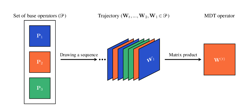
Definition 1 (Multi-view diffusion trajectory -MDT). Let P be a set of transition matrices representing the diffusion operators related to different data-views, and (W i ) i∈N a sequence with W i ∈ P. The operator of a multi-view diffusion trajectory of length t ∈ N * is

Method Row-stochastic Extensible to Tuning of the Real transition matrices more than 2 views time parameter eigenvalues encompassed by MDTs Multi-View Diffusion (MVD) [24] (2020)

✓: offers the feature; ∼: does not scale well with respect to the number of views.

Table 1: Operator-based multi-view diffusion methods. Overview of methods compared to the proposed MDT (and its variants).

Each W i determines the view in which diffusion occurs at step i. Because matrix multiplication is non-commutative, the sequence order defines a specific interaction pattern among views. Intuitively, W (t) describes the cumulative effect of performing t random-walk steps, each possibly performed in a different view. If V = 1, the process reduces to the standard homogeneous diffusion operator P t . For multiple views, however, the process is time-inhomogeneous: the transition law changes with each step, thereby capturing more complex interactions between the views. This flexibility allows the design of different variants of diffusion trajectories by specifying both the composition the set P and the sequence in which the matrix products are applied. Further details on this construction are given in Sec. 3.4.

To ensure that the diffusion process is well-defined for any sequence, we first state simple conditions that guarantee ergodicity and convergence. Proofs are given in Appendix A.

Property 1 (Stability of aperiodicity and irreducibility). If every P ∈ P is a row-stochastic matrix with strictly positive diagonal entries, and the associated Markov chains are aperiodic and irreducible, then any product W (t) obtained from them also defines an aperiodic and irreducible chain.

Therefore, alternating or mixing well-connected views does not break connectivity: the joint diffusion preserves the ability to reach any node from any other in a finite number of steps.

Corollary 1 (Existence of a stationary distribution). Under the same assumptions:

1. Each trajectory W (t) admits a unique stationary distribution π t such that π T t W (t) = π T t .

2. As t→∞, W (t) converges to a rank-one matrix, denoted

Note that, even if W (t) is aperiodic and irreducible, it is generally not self-adjoint in ⟨•, •⟩ 1/πt nor reversible. This corollary says that the inhomogeneous diffusion process converges to a stationary regime, similarly to classical diffusion maps. This implies that the parameter t controls the temporal scale of smoothing: short trajectories emphasize local structure, whereas longer ones capture a form of global organization, common to multiple views. Due to the time-inhomogeneous nature of the process, however, the interpretation of t is more subtle than in the single-view case. In particular, while increasing t generally leads to more global smoothing, different trajectories might yields different rates of convergences, depending on the sequence of views selected. Moreover, the decay of eigenvalues of W (t) might be non-monotonic with t.

Given the MDT operator W (t) , we can define a trajectorydependent diffusion distance that measures the connectivity between datapoints, as determined by the multi-view trajectory at hand. Definition 2 (Trajectory-dependent diffusion distance). Let π t be the stationary distribution of the MDT operator W (t) . The trajectory-dependent diffusion distance between datapoints x i and x j is:

Def. 2 generalizes the standard diffusion distance [3]: two datapoints are close if their transition probability profiles are similar across all views explored by the trajectory, in this sense, this distance is also less sensitive noise inside views, as it aggregates information across their probability profiles. W (t) is not necessarily symmetric or diagonalizable, hence we rely on its singular value decomposition (SVD) to construct an embedding.

The trajectorydependent diffusion map is defined as:

where e i is the i-th canonical vector.

Property 2 (Diffusion distance preservation). The trajectorydependent diffusion map Ψ (t) satisfies:

This embedding preserves the trajectory-dependent diffusion distance, thus generalizing diffusion maps to the proposed time-inhomogeneous process. A key difference from [3] is that they consider the eigenvalue decomposition of P, relying on the direct relation between the eigenvalues of P and P t . In contrast, our MDT operator W (t) is heterogeneous, so the singular q: a quality measure 3: Output: W (t) : a diffusion operator 4: Consider a diffusion operator Pi for each view i 5: Construct the set of base diffusion operators P ▷ see Sec. 3.4 6: Determine a sequence W (t) based on the quality measure q:

values of W (t) are generally not directly related to those of W (t ′ ) for t ′ ̸ = t. Prop. 2 also shows that D W (t) defines a metric on the data points for any t ∈ N * . Moreover, this property enables robust handling of noise via SVD truncation, allowing a balance between preserving the accuracy of the trajectorydependent diffusion distance and reducing the impact of noise in the dataset.

The flexibility of the MDT framework rely on both the definition of P and the selection of the sequence (W i ). In particular, assumptions that are made in the definition of the P are weak enough so that many variations of designs can be explored. We discuss here baseline designs for P, relationship of MDTs with existing multi-view frameworks are further discussed in Sec. 3.5.

A straightforward approach is to define P as a countable set of operators, using either all or a subset of the views.

Definition 4 (Discrete Multi-view Diffusion Trajectory). We say that W (t) is a discrete multi-view diffusion trajectory if for all t, W t ∈ P and P is countable.

A natural choice is to take the canonical diffusion operator set P c = {P v } V v=1 , defined in Sec. 2, where each P v is hte transition matrix for view v. Trajectories may then follow deterministic or random sequences of these operators. When V = 1, we recover the standard single-view diffusion maps. Additional discrete operators can be included in P to enrich the trajectory space: the identity matrix I N allows a ‘idle’ step, the rank-one uniform operator Ξ = 1 N 11 T can introduce teleportation effects when combined with canonical operators as in a PageRankstyle diffusion P PR,v (a) = aP v + (1a)Ξ. While directly taking W i = Ξ collapses the product to rank one, it motivates including teleportation or perturbed operators in more general designs [10]. Similarly, local-scale smoothing operators such as Ξ v = P t ′ v for small t ′ ∈ N * can be added, either directly in P or as replacements for Ξ in PageRank-like operators, to balance local and global diffusion effects [21,10].

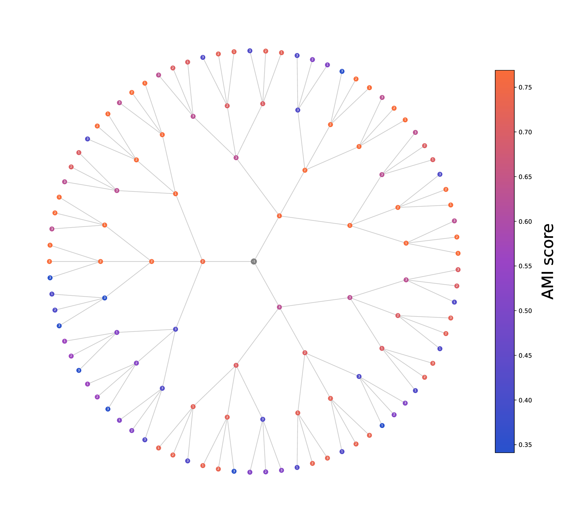
In the discrete setting, trajectories can be visualized as paths in a |P|-ary tree of depth t, where each node at depth i represents the choice of operator W i ∈ P. Consequently, the total number of distinct trajectories grows exponentially with both the number of views V and the diffusion time t, yielding V t possible paths. Fig. 2 illustrates this tree structure for a 3view dataset, with node colors indicating the clustering quality achieved by spectral clustering using the corresponding MDT operators.

Continuous designs. A more flexible approach defines P as a continuous set of operators.

Definition 5 (Continuous Multi-view Diffusion Trajectory). We say that (W i ) i is a continuous multi-view diffusion trajectory if P is continuous. A simple choice is the convex hull of the canonical set (i.e. the convex set including its elements):

The associated MDT operator is then denoted as W (a,t) .

Each convex combination can vary at every step, i.e. a i,v ̸ = a j,v for i ̸ = j. Thus, a trajectory is represented by the sequence of weight vectors (a i ) t i=1 , with V -1 degrees of freedom per step under the simplex constraint. This defines a smooth, continuous search space, enabling interpolation between views and facilitating optimization of trajectories (see Sec. 4.2). As in the discrete case, these convex combinations can include perturbed operators, such as locally smoothed versions of P v , teleportation variants or the rank-one uniform operator, allowing the trajectory to balance local and global diffusion effects.

In fact, this continuous formulation naturally generalizes the classical PageRank random walk: for a single view with P init = {P, Ξ} and using the convex set based of P init , an MDT sequence can be written as

where for all i, a i ∈ [0, 1] and P PR (a i ) = a i P + (1a i )Ξ. To further highlight MDT’s representation capacity, we could consider the aforementioned PageRank extensions that use localscale smoothing operators for each view. In the multi-view case, there will be a set of such smoothing operators to be included, {Ξ i } Vinit i=1 ⊂ P init , whose convex combination would allow W t not only to fuse the transition matrices of the views, but also their associated smoothing operators.

Several existing diffusion map frameworks are recovered as special cases of the proposed MDT framework:

• Alternating Diffusion (AD) [19]: choosing the canonical set and alternating by W i = P (i mod V )+1 , W (V t) yields the alternating diffusion operator at time t.

• Integrated Diffusion (ID) [20]: defining a trajectory where the process first diffuses within each view for t v steps before switching to another, e.g. W (t1+t2) = P t1 1 P t2 2 . Another interpretation is that ID is an AD process on the set of already iterated operators {P tv v |v = 1 . . . V }. ). The space is illustrated as a tree in a circular layout; a trajectory starts from the root, which is the identity matrix, and then navigates in the space by choosing the next operator Wi ∈ P that is added to the product sequence W (t) (Def. 1). The depth of each node indicates the length t of the associated trajectory. Short trajectories emphasize local structure, whereas longer ones capture the global structure, common to multiple views. The tree shows also task-related information: node color indicates the clustering quality (AMI) achieved by spectral clustering using the associated MDT operator.

• PageRank-inspired MDTs: This is one of our designs, which still builds on the well-known PageRank operator to define perturbed multi-view diffusion trajectories. Using convex combinations of the form W i = v a i,v P PR,v (α), this interpolates between view-specific and global diffusion.

Therefore, the MDT framework unifies in a comprehensible way a broad family of operator-based multi-view diffusion methods under a single probabilistic and geometric formulation. In that sense, approaches that construct a composite larger operator than the N × N operators of the views, such as that of [24] (see Sec. 2), do not fall within our framework. The same way, approaches that do not rely on random-walk transition matrices, or uses backward operators such as [40,35], are also outside what MDT can encompass.

One of the most important advantages brought by the MDT framework over the standard approaches, is that it enables operator learning. The space of Multi-view Diffusion Trajectories (MDTs), introduced in Sec. 3, defines a broad family of diffusion operators obtained by combining the view-specific transition matrices contained in P. However, not all trajectories are equally informative: different sequence of view operators (multi-view diffusion trajectories) emphasize distinct aspects of the underlying manifold and propagate different types of interview relations. Importantly, the quality of the resulting embedding depends not only on which operators are selected (P), but also on how they are ordered ((W i )) and on the trajectory length (the number of diffusion steps t). This motivates the definition of an internal quality measure to guide the trajectory selection. Therefore, the search for an ‘optimal’ trajectory is constrained by three elements: i) the expressiveness of P, ii) the diffusion time t, and iii) the chosen task-dependent quality measure. This section formulates the selection, or learning, of diffusion trajectories as an optimization problem guided by a suitable internal measure, which seeks for effective optimization strategies to deal with the constraints introduced by the MDT framework.

Given a dataset represented by the operator set P, the objective is to determine a sequence of matrices τ = (W i ) t i=1 who’s product W (t) produces a meaningful (for the problem at hand) and well-structured embedding of the data. This search is guided by an internal quality measure Q(τ ), defined as:

where P t is the set of all possible sequences of length t formed by the operators in P. Although t is a parameter in the problem formulation, in practice it is often fixed using heuristics [20]. We will showcase later on how to adapt such heuristics to the MDT framework. Typical internal measures include clustering validity indices such as the Davies-Bouldin, Silhouette, and Calinski-Harabasz (CH) indices [38,6], which have all been extensively studied (e.g. see [9]). Without relying on external labels, such indices can evaluate the compactness and separation of clusters formed in the diffusion space [33,34], which in the present case would be induced by a trajectory, and there-fore can serve as guiding internal quality measures. Each index introduces its own bias, reflecting specific assumptions about what constitutes a ‘good’ clustering, and should therefore be selected and interpreted with care. Although originally defined for single-view settings, a simple way to be extended to the multi-view case is by computing a weighted sum of the perview scores, where the weights account for both the relative importance of each view and the scale of the corresponding criterion. In Sec. 5.3, the CH index is adopted as the internal quality measure Q(τ ) evaluated on the diffusion operators {P i } V i=1 . CH is a computationally efficient index that has been shown to perform well in various clustering scenarios [6]. For a dataset X and a clustering C, the CH index is defined as:

where C i (τ ) is the clustering obtained by applying k-means on the trajectory-dependant diffusion map obtained by τ , B C and W C are the between-and within-cluster scatter matrices, respectively, and w i is a weight associated to view i that is set to w i = 1/V in the absence of prior knowledge. Other single-view clustering validity indices can be used in place of CH within the definition of Q • (τ ). In Sec. 5.2, we alternatively propose and employ a contrastive-inspired internal criterion to assess the quality of the learned embeddings.

The optimization strategies discussed in this section aim to select or learn effective diffusion trajectories within the MDT framework. To do so, they rely on either the continuous or the discrete MDT formulation, defined in Sec. 3.4. This section’s strategies are summarized in Tab. 2.

Random sampling. We first consider selecting diffusion trajectories through random sampling as a simple and computationally inexpensive baseline. This approach provides a reference distribution over trajectories that captures the average random behavior of multi-view diffusion without explicit optimization, and without relying on an internal quality measure, serving as a useful baseline to assess the impact of more sophisticated trajectory designs.

Definition 6 (Random multi-view trajectory). A sequence of operators (W i ) i∈N is called a random multi-view trajectory if each operator W i is independently drawn from a probability distribution µ i supported on the operator set P:

This stochastic process can be viewed as a discrete-time Markov Jump Process (MJP) [4], where the states correspond to the operators in P and the transition law evolves according to the sequence of distributions (µ i ) i . When for all i, µ i = µ, then W i i.i.d.

∼ µ, and the resulting expected operator satisfies

t , which represents the average diffusion geometry induced by random sampling. Although individual trajectories may yield noisy embeddings, the ensemble of such random paths approximates a mixture model over all possible diffusion trajectories. This property makes random sampling valuable as an unbiased baseline and as a stochastic regularization mechanism; this aspect is further developed in Sec. 5. In practice, this approach enables fast generation of multiple trajectories at negligible cost, providing an empirical evaluating reference.

Criteria-based selection. Using the problem formulation in Sec. 4.1, we can establish criteria for selecting promising trajectories based on their expected performance according to the chosen task-dependent quality measure Q. Depending on the trajectory space, different optimization strategies can be employed. In the discrete MDT setting, tree search algorithms can efficiently explore the combinatorial space of operator sequences. Techniques such as beam search, Monte Carlo Tree Search or ε-greedy algorithms can be used to select MDTs that achieve higher quality scores. In the continuous MDT setting, gradient-based optimization methods or evolutionary algorithms can be utilized to navigate the continuous parameter space defined by P. In the particular case of a convex MDT, where the operator is expressed as a convex combination of the form W i = Vinit v=1 a v P v , these optimization methods refine iteratively the weight vectors (a i ) to maximize the quality index Q, potentially uncovering nuanced combinations of views that better capture the underlying data structure. The choice of optimization strategy should consider both computational efficiency and the ability to escape local optima, ensuring a robust search for high-quality diffusion trajectories. In particular, for this purpose we consider Direct [18], which has the advantage of being non-stochastic and hence has needs lower computational cost compared to stochastic methods, but works well when t×|P init | is relatively small. Other methods can also be considered for the optimization, e.g. [15,32,25,17].

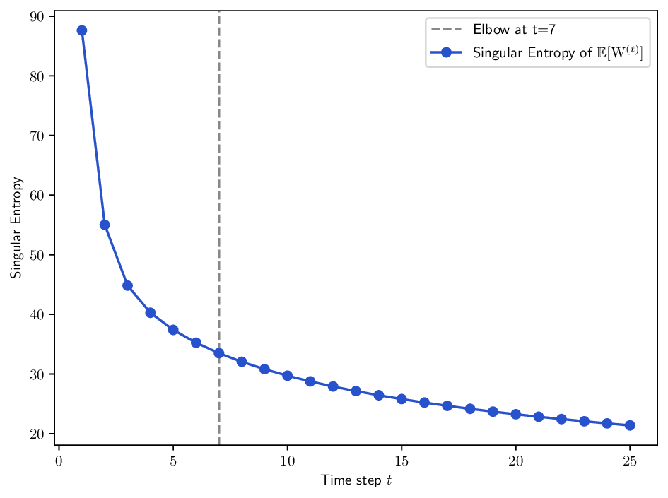
Selecting the diffusion time horizon (t). The number of diffusion steps t is a critical hyperparameter that controls the scale at which the data structure is analyzed: short diffusions emphasize local geometry, while longer ones over-smooth the manifold and eliminate fine details. For determining t, we adapt an existing approach that tracks how the singular value spectrum of W (t) evolves over time [20]. To this end, we define the singular entropy as the Shannon entropy of the normalized singular value distribution:

where the singular values are normalized to

Low entropy indicates that most of the diffusion energy is concentrated in a few leading components (i.e. the matrix is close to rank-one), suggesting that the dominant structure has emerged. High entropy reflects a more uniform spectrum, potentially corresponding to noise or unresolved substructures. The optimal diffusion time is chosen at the elbow point of the entropy curve, balancing noise reduction and information retention.

Although W (t) converges to a rank-one matrix asymptotically (Corollary 1), its singular values do not necessarily decrease monotonically due to the inhomogeneity of the process. To mitigate fluctuations, we compute the entropy of the expected operator E µ [W (t) ] that yields smoother and more stable behavior in practice. When no prior information about the relative importance of views is available, the expectation is taken under an i.i.d. assumption with uniform measure µ = 1 |P| over P. In this context:

This section showcases the proposed MDT framework in the manifold learning and the data clustering tasks. We define the MDT variants presented in Tab. 2, which derive from the proposed MDT framework (Sec. 4). In the manifold learning context, we employ the convex MDT-CST that is obtained by optimizing a contrastive-like loss (Sec. 5.2). In the clustering case, we choose the Calinski-Harabasz index (CH) as an internal clustering-based quality criterion to guide the MDT construction. Four MDT variants are considered for clustering: MDT-RAND, MDT-CVX-RAND, MDT-DIRECT, and MDT-BSC (Sec. 5.3). MDT-RAND and MDT-CVX-RAND represent randomly sampled trajectories in discrete and convex spaces, respectively. MDT-DIRECT employs Direct optimization in the convex set P cvx , while MDT-BSC uses beam search to explore the discrete trajectory space P c . We then compare against state-of-the-art multi-view diffusion methods, (Sec. 2.2, Tab. 1). The performances of single-view diffusions are reported in Appendix . Since identifying the best view in an unsupervised manner is generally not feasible, these single-view results are included only as references to contextualize the performance of multi-view methods.

For methods requiring a time parameter tuning (ID, MDT-RAND, MDT-DIRECT, MDT-CVX-RAND, and P-AD), we use the elbow of the singular/spectral entropy using the Kneed package [30], while for MDT-BSC, the maximum width of the tree is set to 2 times this elbow. CR-DIFF does not come with a tuning mechanism for the time parameter, hence we follow the suggestion of its authors to set a high value of t = 20. In the other cases, the time parameter is set to t = 1. Multi-view diffusion MVD produces one embedding per view, since no specific view is preferred, we report the embedding associated to the first view.

In the following subsections, we present results obtained on toy examples and real-life datasets whose characteristics are summarized in Tab. 3. We consider point-cloud data, and the transition matrices are built using Gaussian kernels with bandwidth σ = max j (min i,i̸ =j dist v (x i , x j )), with dist v denoting the Euclidean distance in view v. A K-nearest neighbors (K-NN) graph is then constructed on the kernelized data (K = ⌈log(N )⌉). In the manifold learning setting, the embedding dimension is fixed to 2 to facilitate visualization. In clustering experiments, the dimensionality of the embedding space is set equal to the number of target clusters (k), which is assumed to be a known hyperparameter. The implementation of the MDT variants and all the compared methods has been included in an open-source repository2 .

Internal quality index. To learn MDTs for this task, we propose the following quality index to guide the process, inspired from recent works on contrastive learning [28,14]:

where

denotes the neighbors of node i in view v (determined by the kernel matrix, generally after a K-NN step), and λ v is a weighting parameter representing the relative view importance. W (a,t) is an MDT operator associated to the convex set P cvx (see Def. 5). For convenience, we set λ v = 1/v for all v, and choose t using the heuristic defined in Sec. 4.2. To optimize with regards to the proposed loss, we employ the ADAM optimizer. This configuration is named as MDT-CST.

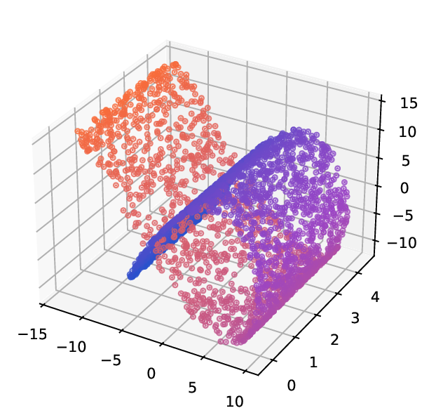
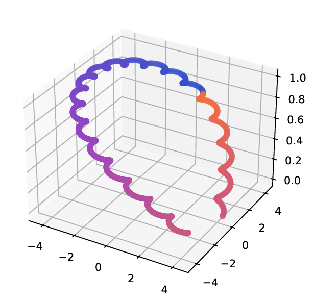
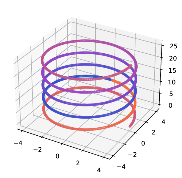
Datasets. Helix-A and Helix-B [24] are two synthetic datasets used to evaluate manifold learning algorithms, as they present challenges in capturing the underlying geometry of the data from multiple perspectives . They consist of n = 1500 points sampled from a 2D spherical structure. The points are then embedded into a 3D space using two different nonlinear transformations, resulting in two distinct views. Helix-A’s datapoints are generated as x i = {x i,1 , x i,2 } n i=1 , where x i,1 are evenly spread in [0, 2π) and x i,2 = x i,1 + π/2 mod 2π. View 1 and view 2 are generated by Φ 1 and Φ 2 , respectively, those deformations are defined as follows; for i ∈ {1, …, n}:

Helix-B stems from the previous one, where the definition of the views rely on the same input points {x i } n i=1 . The transformations are defined for i ∈ {1, …, n} as:

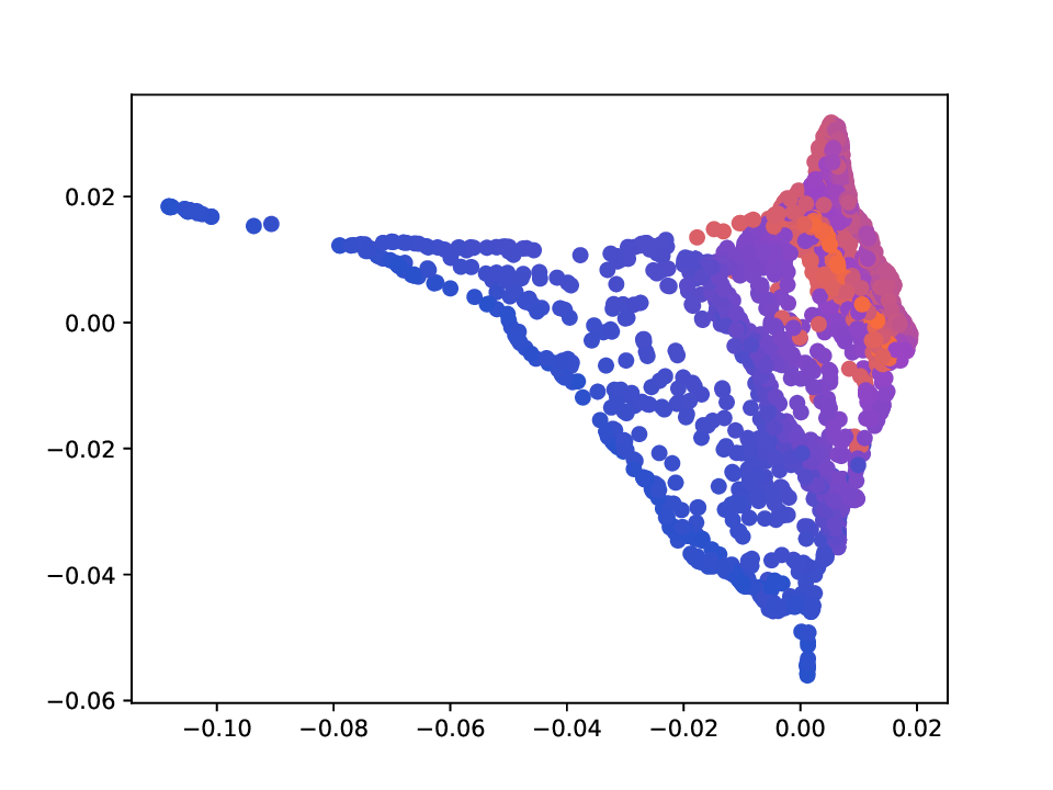
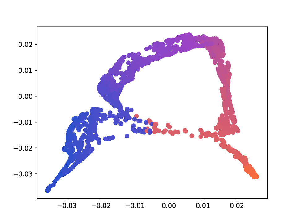
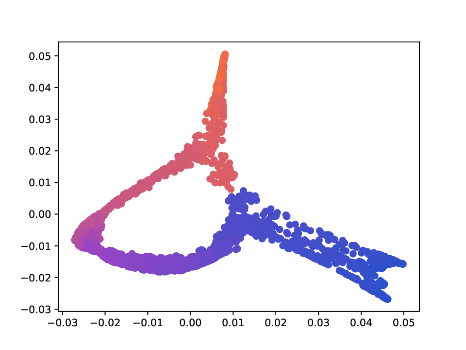
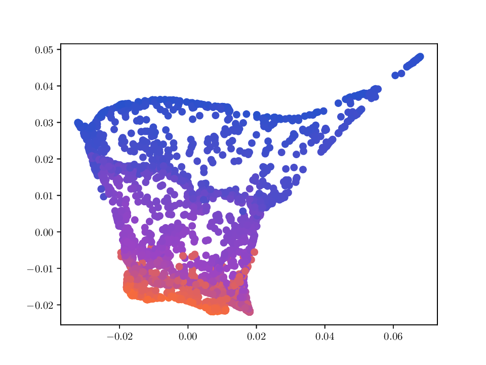
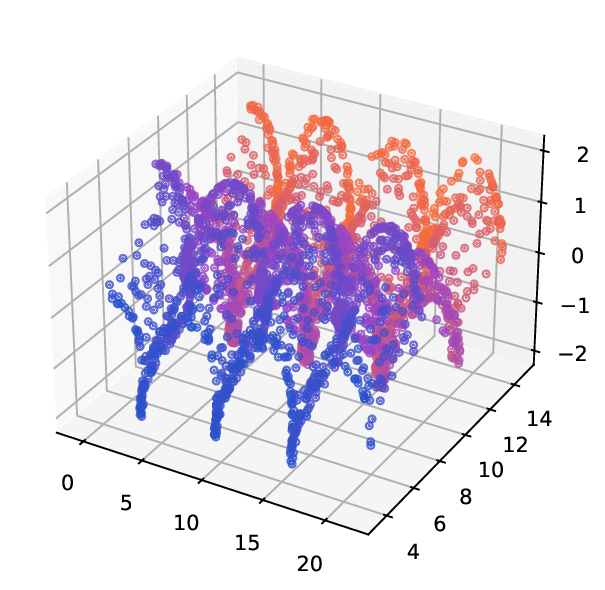
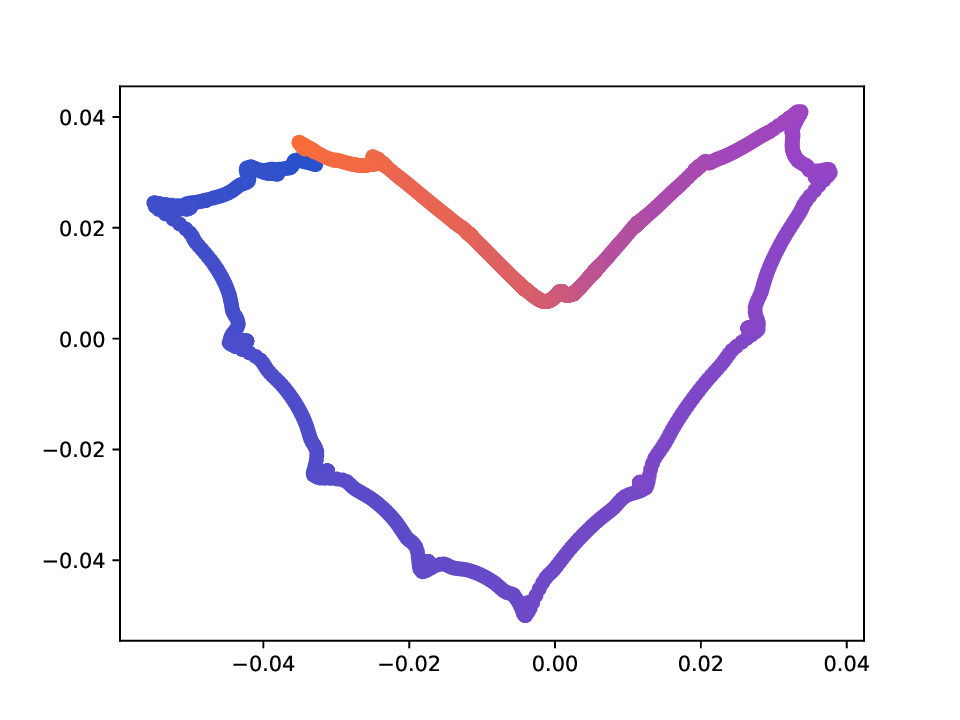
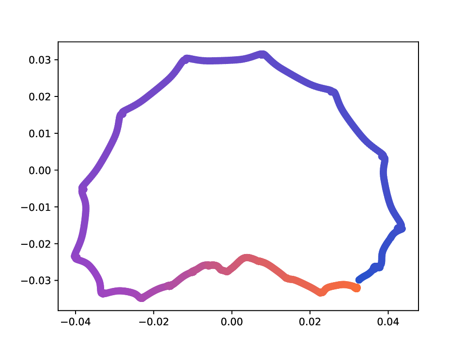
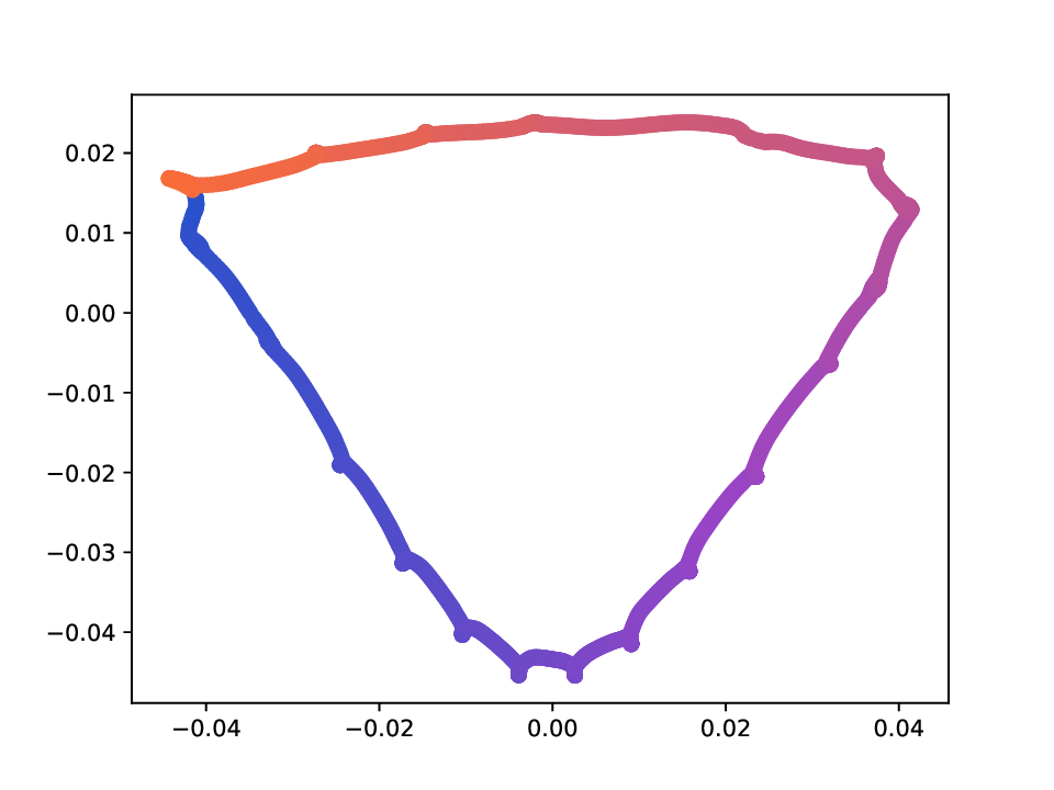
x i,1 The Deformed-Plane dataset consists of points originally sampled uniformly on a plane. The plane is then deformed by two non-linear, non-bijective transformations that introduce connectivity not present in the original flat plane. Fig. 5 shows a visualization of this dataset. Specifically, points x = (x 1 , x 2 ) ∈ R 2 are sampled as x 1 ∼ U(0, 3π/2) and x 2 ∼ U(0, 21), and two views are generated via the transformations Φ 1 and Φ 2 , defined by

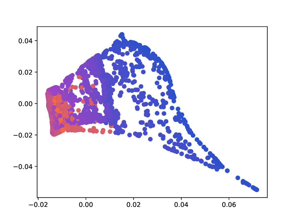
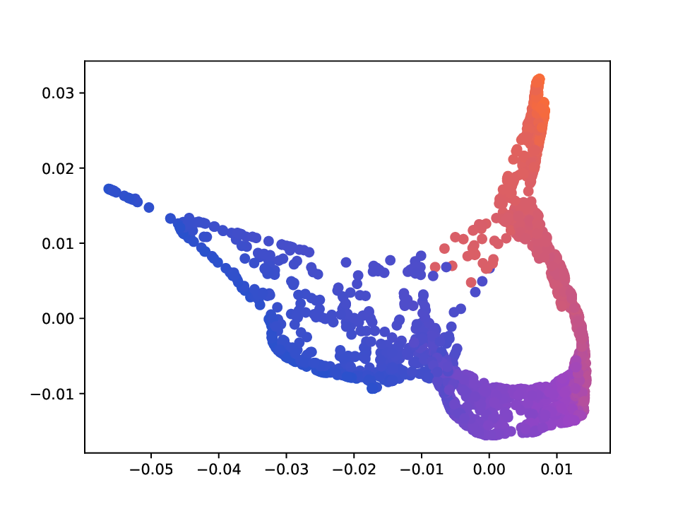
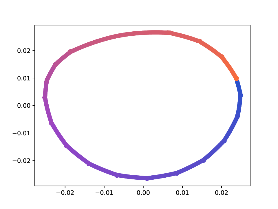
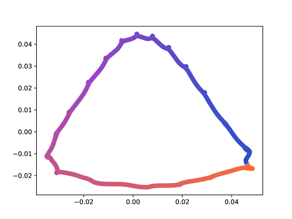
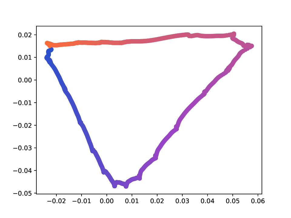
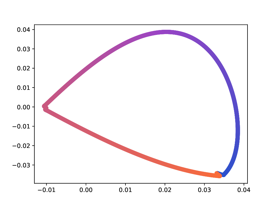
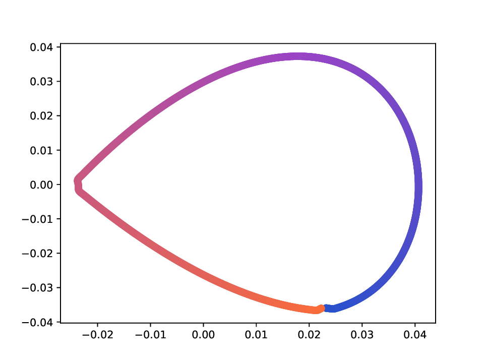
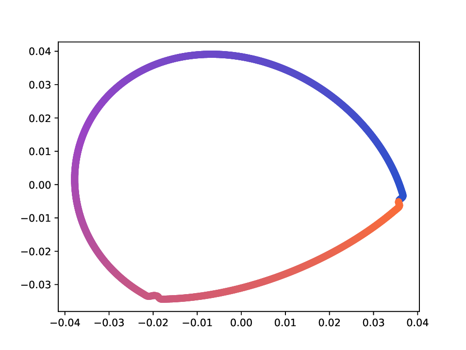
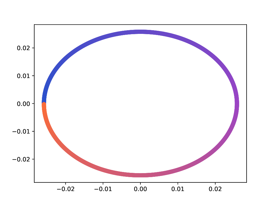
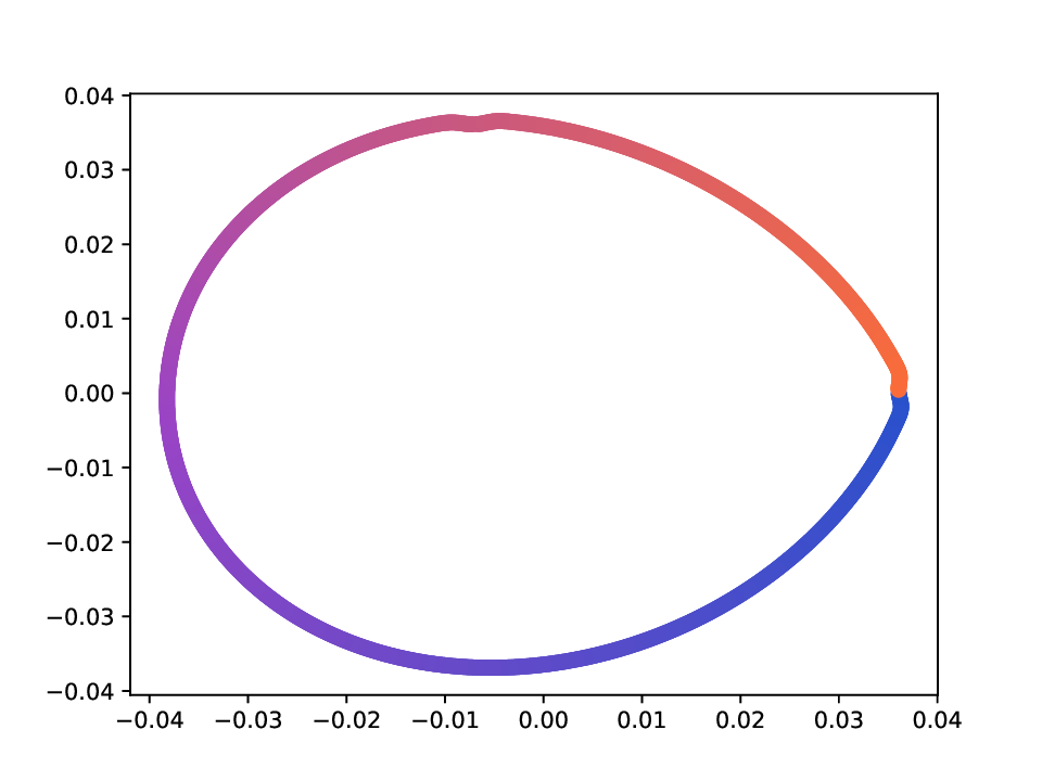
Results. For the Helix-A and Helix-B datasets, the compared methods are used to generate two-dimensional embeddings of the original 3D helices. The resulting embeddings are shown in Fig. 3 and Fig. 4. In both cases the embeddings produced successfully capture the circular structure of the underlying manifold. Specifically, methods that rely on the eigen-decomposition tend to produce smoother embeddings that the ones relying on the SVD of the operator. This is particularly seen in the case of the Helix A dataset, where MVD produces a very smooth embedding, while AD produces a pointy one. Those datasets serve as sanity checks for the multi-view manifold learning task.

For the Deformed-Plane dataset, both views exhibit clear limitations when attempting to recover the original underlying manifold. This highlights that combining these views requires careful consideration, leveraging only the parts of each view that are believed to be accurate. However, due to these inher-ent limitations, no view can perfectly recover the original manifold structure, as the transformation from the original manifold to the observed representation is non-bijective. The results for this dataset are presented in Fig. 5. MVD and AD struggle to recover the underlying manifold, resulting in significant overlap between regions that should be distinct. ID captures an embedding with an ‘omega’ shape, effectively capturing the connectivity of the original manifold, although a slight overlap between the orange and blue points exists. Randomly sampled MDTs produce similar embeddings, also showing strong overlap, except for the fourth case that produces a representation without any overlap. Two embeddings produces by MDT-CST are shown, one using the time parameter t = 1, and another using t = 8. Both recover representations that are ‘meaningful’. When using t = 1, we obtain a representation that admits no overlap between the regions, but where the blue and orange regions are mapped close to each other. In the case of t = 8, those regions are better separated, at the cost of a slight overlap.

Overall, the results highlight the merits of MDT and the advantages of using the proposed contrastive loss for trajectory optimization in multi-view manifold learning.

External and internal quality indices. When true class labels are available giving the true class of the datapoints in a benchmark dataset, the quality of a produced clustering partition can be evaluated through supervised measures. We specifically use the Adjusted Mutual Information (AMI) measure [39], which is adjusted for the effect of agreement due to chance. Higher AMI values are preferred as they indicate partitions that match better with the partition that is induced by the true labels. We report (e) ID embedding; (f) embeddings obtained using four random MDTs; (g) the MDT embedding obtained using a trajectory optimized for QX . -Methods that are based on the SVD of their related diffusion operator (AD, ID, and MDTs) produce less smoothed embeddings compared to MVD, which relies on the eigendecomposition. This is particularly evident in the case of AD, which generates a pointy embedding. However, all methods seems to recover the circular structure of the underlying manifold in a rather meaninful manner. Moreover, we can observe that the embeddings obtained from randomly sampled MDTs are similar, indicating that many trajectories in this case lead to satisfactory embeddings. -Both MVD and AD struggle to recover the hidden manifold, with significant overlap between regions that should be distinct. ID captures an embedding with an ‘omega’ shape, essentially capturing the connectivity of the original manifold, although a slight overlap between the orange and blue points exists. The embeddings from randomly sampled MDTs are diverse, including a case (bottom-right in (f)) that exhibits no overlap, and others with strong overlap. By contrast, optimizing the proposed criterion QX yields a representation closer to the original manifold. At t = 1, there is no overlap between regions, but the orange and blue regions are close to each others. At t = 8, though, those regions are better separated, at the cost of a slight overlap.

the average value and standard deviation of those measures over 100 runs of a clustering method in each case.

Regarding the learning of MDTs, an internal quality index is needed to guide the process. Each such internal index imposes its own bias, in particular, optimal partitions according to a given index may not align with the optimal partition according to another index. As stated in Sec. 4, we consider the Calinski-Harabasz (CH) index [6], which is a widely used internal clustering validation measure. The CH index evaluates the quality of a clustering partition by considering the ratio of betweencluster dispersion to within-cluster dispersion. Higher CH values indicate better-defined clusters, as they reflect a larger separation between clusters relative to the compactness within clusters. When learning MDT trajectories for clustering, we aim to maximize the CH index. An analysis of the correlation between AMI and CH on real-life datasets (see details in Appendix B) shows that optimizing CH generally leads to improved AMI scores, although this relationship is not strictly monotonic.

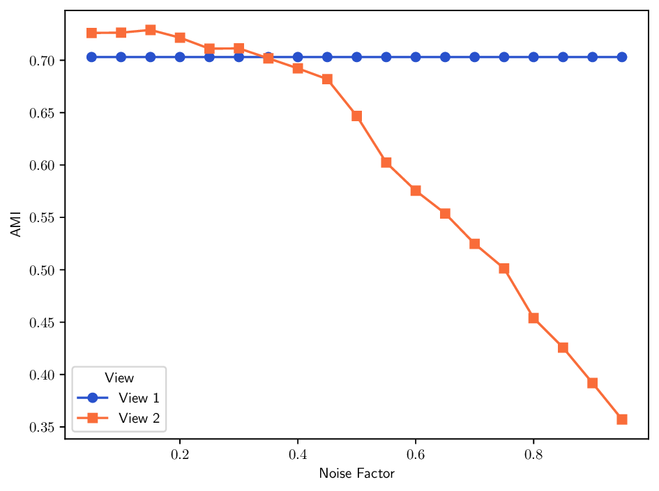
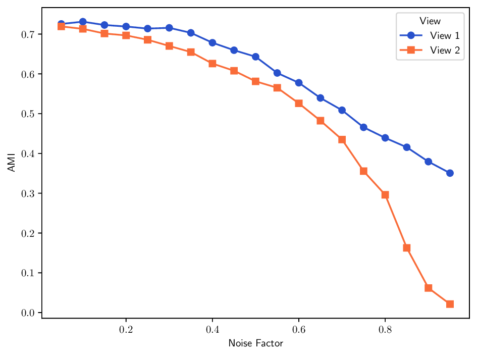
Datasets. The Multiple Features dataset (Multi-Feat) contains 2000 handwritten digits that are extracted from Dutch utility maps 3 . Each digit is represented using six distinct feature sets: Fourier coefficients of the character shapes, profile correlations, Karhunen-Loève coefficients, pixel averages in 2 × 3 windows, Zernike moments, and morphological descriptors. K-MvMNIST [20] and L-MvMNIST [24] are two multiview variants of the MNIST dataset, which are inspired by prior work. K-MvMNIST has 2-views, one consist of the original images with an added fixed Gaussian noise N(0, 0.3), and the other view is obtained by adding a different Gaussian N(0, s), where s ∈ [0, 1) is a robustness parameter. The impact of the second Gaussian noise on clustering results is shown in Fig. 7a. L-MvMNIST follows a similar setup, it defines a robustness parameter s ∈ [0, 1), then the first view is created by adding Gaussian noise N(0, s) to the original image, the second view by randomly dropping each pixel with a s% probability. Unlike prior work [24] that used only digits 2 and 3 drawn from the infiniMNIST dataset, we use here the original MNIST dataset, downsampled to 6000 samples. In both cases we set by default s = 0.5, while the importance of this parameter is analyzed in Fig. 7a and Fig. 7b.

The L-Isolet dataset [24] is a multi-view dataset generated from single point-cloud view using different kernels. Its 1600 datapoints are observed in either 3 views:

, where T ij is the correlation between x i and x j , and σ follows the max-min heuristic. This dataset evaluates whether clustering methods can detect informative kernels and merge heterogeneous structural information.

3 UCI repository at: http://archive.ics.uci.edu/dataset/72/multiple+features .

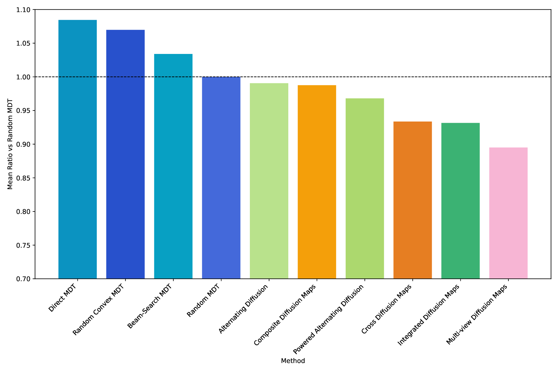
The next five datasets are all available online4 . • The Olivetti dataset consists of grayscale facial images represented through two feature descriptors: a HOG transform of the datapoints, and a 150 principal component analysis (PCA) representation, offering complementary texture and structural information. • Yale faces dataset consists of 165 gray-scale face images belonging to 15 subjects with each subject containing 11 images. Each image is represented using three feature sets: a Gabor filterbased descriptor, a Local binary patterns feature, and a raw pixel intensity vector. • The 100leaves dataset is multi-class dataset where each leaf sample is characterized through several shape and texture-oriented feature views, capturing different morphological aspects of the same object. In particular, three views are used: shape descriptors, fine scale margin and texture histogram. Random MDTs as a baseline. Beyond their mere performance, MDTs also provide a valuable baseline tool for analyzing multiview diffusion behavior. Since the MDT framework is general and parameterized only by the operator set (P) and the optimization strategy to determine a trajectory, one can instantiate MDTs with minimal assumptions to check how view interactions influence learning outcomes. In this sense, MDT-RAND can serve as a ’neutral’ diffusion baseline: random or uniformly sampled trajectories represent an unbiased mixture of views, while convex or optimized variants reveal how adaptive view weighting affects manifold recovery or clustering. Through this lens, MDT-RAND constitutes a principled and interpretable reference point for evaluating multi-view fusion strategies, which is particularly useful for diagnostic or benchmarking purposes, e.g. when assessing the sensitivity of downstream tasks to the order or frequency of cross-view diffusion. To employ this idea we introduce the Performance Ratio to Random (PRR) index, which is the AMI ratio of a method to the MDT-RAND baseline in the canonical set P c , which treats all views and their combinations evenly. The average PRR across datasets is reported in Fig. 6 Each bar shows the PRR index (Eq. 21), which is the ratio of the AMI obtained by a method to that obtained by MDT-RAND. Ratio values below 1 indicate worse average clustering performance than MDT-RAND, while values above 1 indicate better performance. The results highlight that the three first designed MDT variants outperform the plain random MDT-RAND counterpart, all other diffusion-based methods, some of which encompassed by the MDT framework, come after and importantly they do not perform better than our MDT-RAND baseline.

AMI and standard deviation. Additional analysis on the noisefactor-based datasets is given in Figs. 7a and7b. Comparative performance. In Tab. 4, MDT variants based on the convex set P cvx (MDT-CVX-RAND, MDT-DIRECT) consistently achieve strong clustering performance across datasets, often outperforming established methods such as MVD, AD, P-AD, and ID. This underscores the importance of carefully designing P for MDTs’ success. Notably, MDT-DIRECT attains the highest AMI on five of the nine datasets and ranks second on one. Although MDT-CVX-RAND does not achieve the top score on any dataset, it performs consistently well, suggesting that convex interpolation of views provides a robust strategy. As MDT-BSC can evaluate trajectories of varying lengths, it can adaptively select diffusion scales for each dataset, which is advantageous when a fixed diffusion time heuristic fails to capture the appropriate scale. However, this flexibility can re- sult in sub-optimal choices, notably when the internal criterion doesn’t align with the ground-truth labels, as illustrated by the 100Leaves dataset, where MDT-BSC underperforms noticeably.

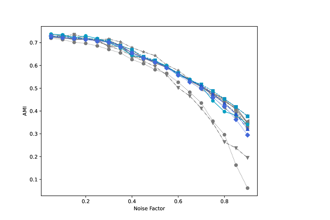
Overall, these results highlight the flexibility and effectiveness of the MDT framework when paired with thoughtfully designed trajectory spaces and optimization strategies. Looking at the PRR index in Fig. 6, we observe that the three first designed MDT variants outperform the plain random MDT-RAND counterpart, all other diffusion-based methods, some of which en-compassed by the MDT framework, come after and importantly they do not perform better than our MDT-RAND baseline. This further emphasizes the strength of the MDT framework and the importance of trajectory design. Robustness to noise. Fig. 7 illustrates how different methods behave as the noise factor s increases. In K-MvMNIST, only the second view is affected by noise, so methods that treat both views equally show a faster decline in performance compared to those employing weighting strategies (e.g., ID, MDT-CVX-RAND, MDT-BSC), which seems to attain similar performance decay with the addition of noise. In L-MvMNIST, the quality of both views deteriorates substantially with increasing s, and all methods experience a corresponding drop in AMI scores.

These experiments demonstrate the robustness of MDTs when paired with appropriate trajectory designs and optimization strategies: they can leverage the more informative views while reducing the impact of noisier or less reliable ones.

This work introduced Multi-view Diffusion Trajectories (MDTs), a unified operator-based framework for constructing diffusion geometries across multiple data views. By modeling multi-view diffusion as a time-inhomogeneous process driven by sequences of view-specific operators, MDTs generalize a family of existing multi-view diffusion methods, including Alternating Diffusion and Integrated Diffusion, while offering significantly greater flexibility. In that sense, our framework provides a common language in which these methods can be analyzed, compared, and extended.

We established fundamental properties of MDTs under mild assumptions and formulated trajectory-dependent diffusion distances and embeddings via singular value decompositions of the induced operators. This provides a principled extension of classical diffusion maps to settings where the diffusion law evolves over time. The proposed trajectory space further enables, for the first time, operator learning within diffusion-based multi-view fusion, opening an avenue for view-adaptive diffusion processes that can selectively emphasize complementary structures across views.

Empirical evaluation on both manifold learning and clustering tasks shows that MDTs are expressive and practically effective. Both discrete and convex variants achieve competitive or superior performance compared to established multi-view diffusion approaches, showing the benefit of structured operator sequences over fixed fusion rules. Notably, randomly sampled trajectories (MDT-RAND), relying only on a chosen time parameter, achieve high performance, highlighting the richness of the MDT operator space and indicating that even simple exploration strategies can yield informative multi-view geometries. Moreover, MDT-RAND serves as a useful baseline for evaluating diffusion-based multi-view methods, as it is not consistently outperformed by more sophisticated approaches in practice.

Overall, MDTs provide a coherent, extensible, and computationally tractable framework for multi-view diffusion. Their flexibility in operator design and compatibility with principled learning criteria make them a powerful foundation for future developments in multi-view representation learning. The unified view offered by MDTs can guide the design of new multiview diffusion models and contribute to a deeper understanding of how heterogeneous data sources can be fused through iterative geometric processes. Potential directions include integrating supervised objectives into trajectory learning, improving scalability via graph sparsification, and exploring connections with neural or contrastive graph-based methods. Exploring continuous-time MDT formulations, could underpin strong connexions analogous to heat kernels. = (e ie j ) T Ψ (t) 2 .

(A.

The 4-th equation comes from the fact that, by definition of an SVD, N is semi-orthogonal matrix, thus x T N T 2 = ∥x∥ 2 by the isometry property.

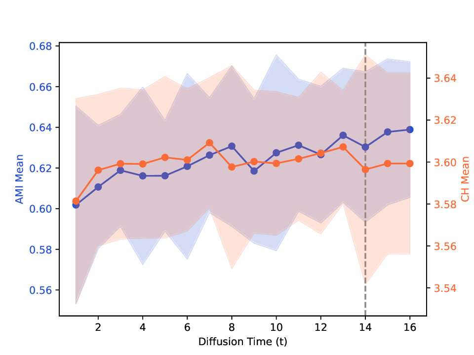
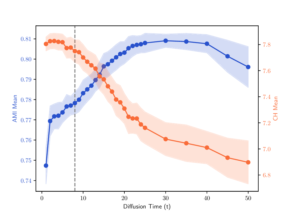
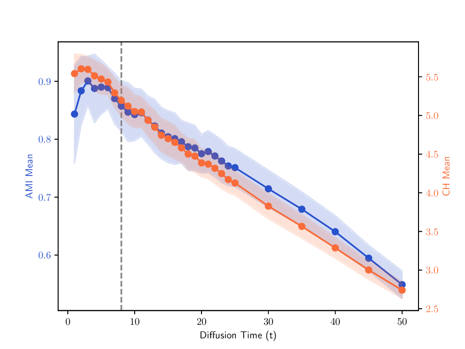
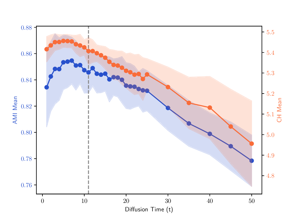
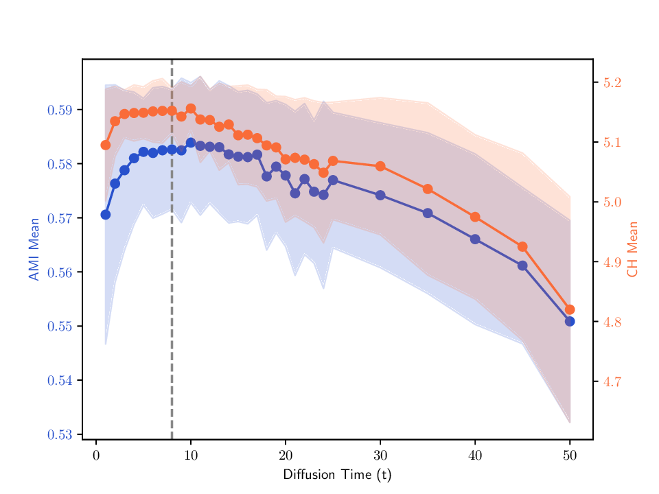
Singular entropy of the expected random trajectory. As we use the elbow of the singular entropy curve to select the t parameter, we provide in Fig. B.8 the singular entropy curves for the expected random trajectory on two different datasets used in Sec. 5. The same exponential decay behavior is observed on all datasets, and the selected t parameter (elbow point) is indicated by a vertical dashed line.

Correlation between internal criterion and clustering quality. We examine two aspects of the relationship between the internal criterion (CH index) and clustering quality as measured by AMI. First, Tab. A.5 reports the CH scores for the groundtruth labels alongside those produced by the evaluated methods, allowing inspecting how closely the internal criterion matches the actual clustering structure. Second, Fig. B.9 shows how the CH and AMI vary with trajectory length, where we plot both metrics for randomly selected MDTs in P cvx and track how their averages evolve over time. This showcases how optimizing CH may impact AMI, and reveals how MDTs’ clustering quality is affected by the choice of trajectory length. The figure also marks the time parameter adopted in Sec. 5.3, which typically falls in a region where both AMI and CH are high. Although not always optimal, this tuning is a reasonable compromise that clearly avoids ranges associated with low AMI.

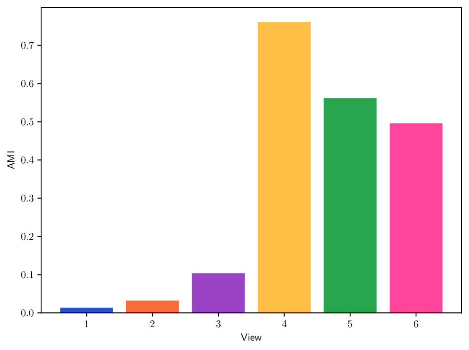
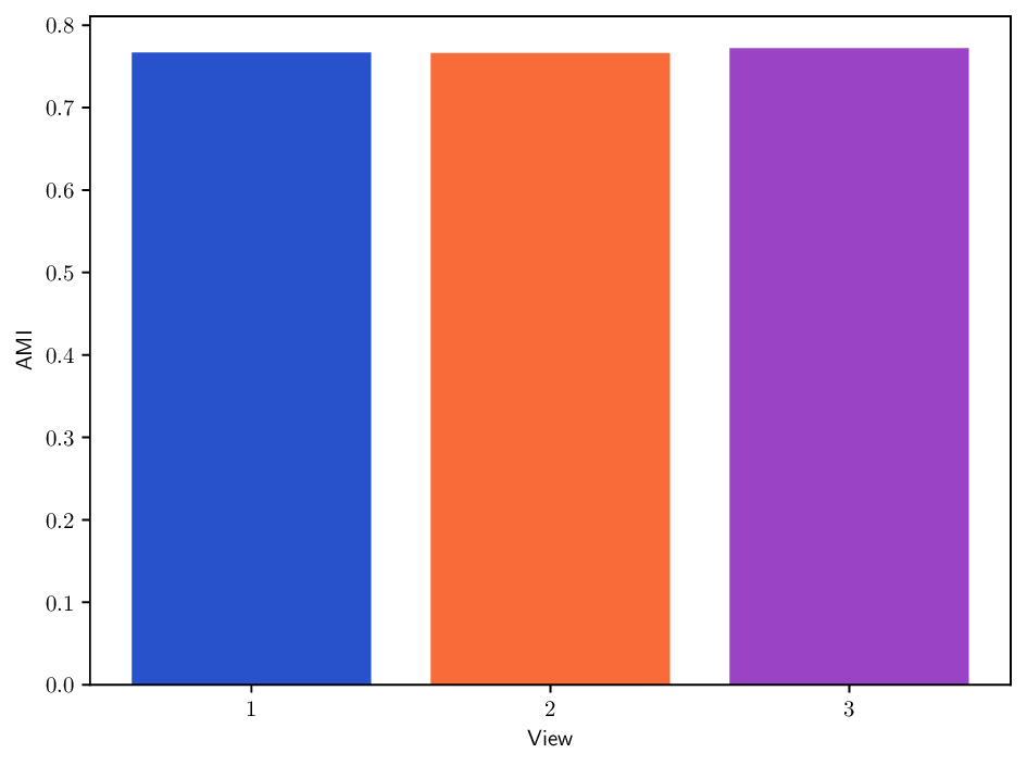
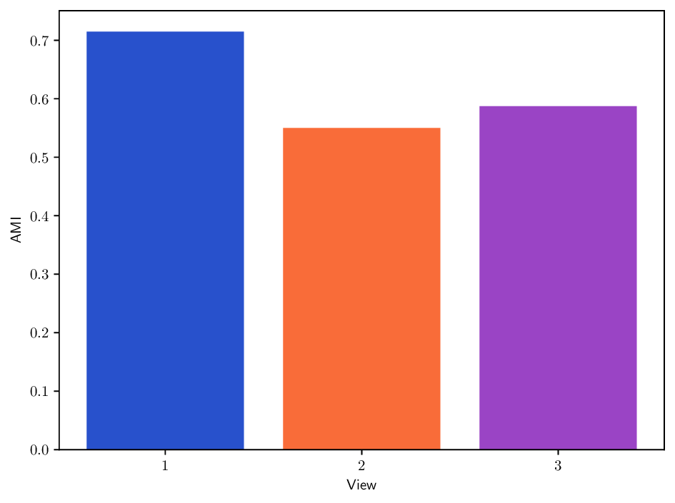
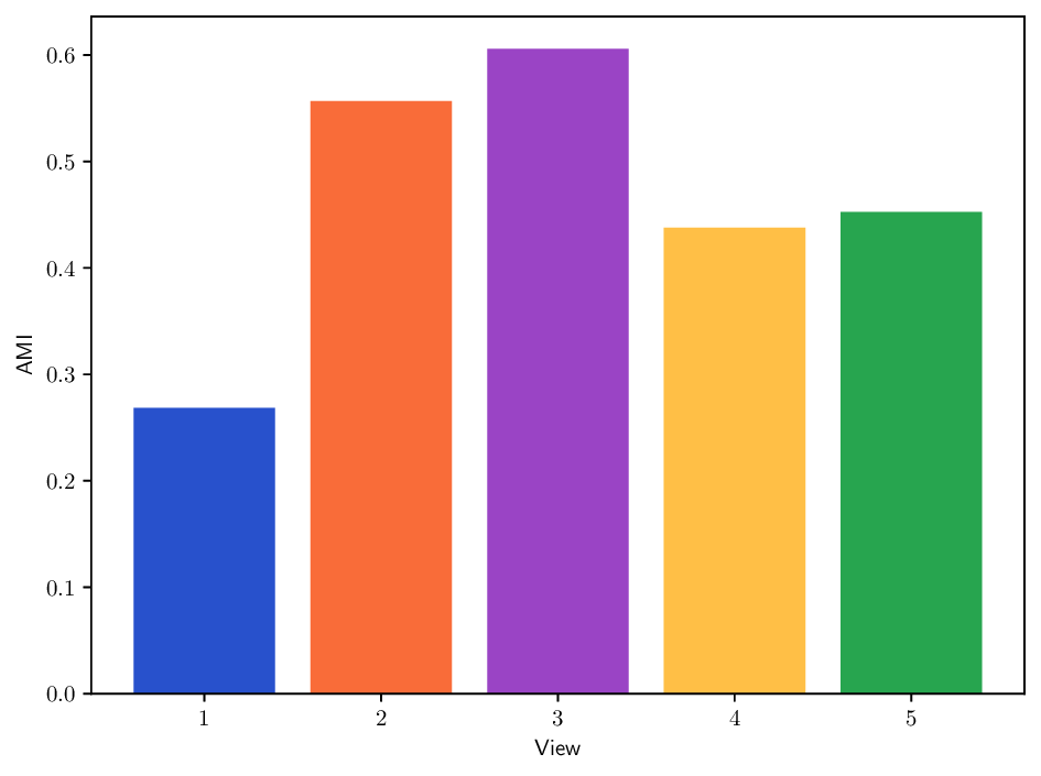
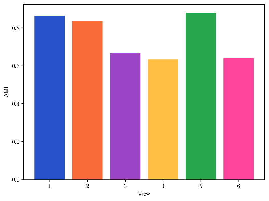
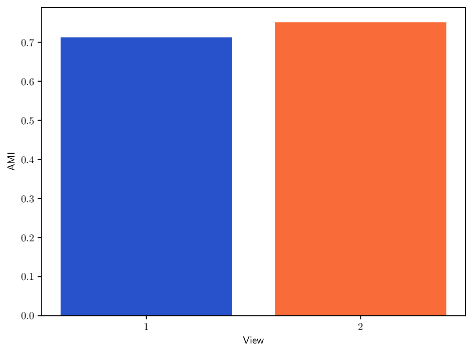
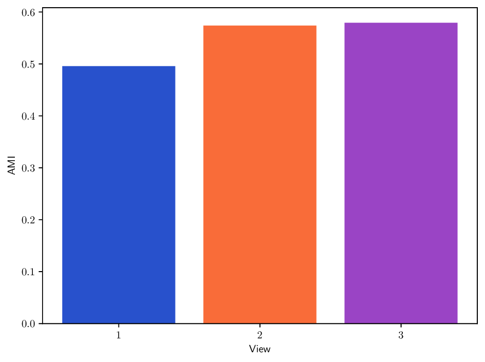
Reference clustering quality per view. To better understand the clustering performance of different methods on multi-view datasets, we report in Fig. B.10 clustering results (AMI) achieved when using each individual view separately. This analysis provides insights about how informative each view is and how it may contribute to the overall clustering performance for each method. In particular, we can see that the Caltech101 dataset admits a strong heterogeneity in view quality, with view 1-3 being significantly less informative. Similarly, in K-MvMNIST

  , and Φ 2 (x) = 4

2 = (e ie j ) T Π -1/2 t MΣ t N T 2 = (e ie j ) T U t Σ t 2

Iterating row-stochastic matrices: If P and Q are two row-stochastic matrices, the product PQ T is not generally stochastic: j (PQ T ) ij = j,k P ik Q jk = k P ik ( j Q jk ), which sums to 1 only if j Q jk = 1 for all k. This holds only when Q is doubly stochastic, which is not assumed here.

The repo is available at: https://github.com/Gwendal-Debaussart/mixed-diffusion-trajectory

Olivetti is available online at: https://www.cl.cam.ac.uk/research/dtg/attarchive/facedatabase.html; the four other datasets are available at: https://github.com/ChuanbinZhang/Multi-view-datasets/

📄 Read Full PDF on ArXiv

This content is AI-processed based on open access ArXiv data.