Differentiable Weightless Controllers: Learning Logic Circuits for Continuous Control

1 ISTA (Institute of Science and Technology Austria), 3400 Klosterneuburg, Austria. Correspondence to: Fabian Kresse fabian.kresse@ist.ac.at. However, policies implemented as neural networks rely on large numbers of compute-intensive multiply and accumulate operations, making their applications on resourceconstrained hardware platforms, such as UAVs and mobile robots, difficult. In such cases, policies implemented as small and discrete-valued functions are preferable, as these allow efficient implementation on embedded hardware, such as FPGAs.

Because low-precision floating point or integer-only operations have efficiency advantages even on high-end GPUs, several prior works have studied either converting standardtrained deep networks into a quantized representation (posttraining compressions, PTQ), or learning deep networks directly in quantized form (quantization-aware training, QAT), see e.g. Gholami et al. (2022) for a recent survey. However, most such works target a static supervised or next-wordprediction setting, in which the input and output domains are discrete to start with, and the task involves predicting individual outputs for individual inputs.

The setup of continuous control, i.e. learning control policies for cyber-physical systems such as autonomous robots or wearable devices, is more challenging, because input states and output actions can be continuous-valued instead of categorical, and the controller is meant to be run repeatedly over long durations, such that even small errors in the control signal might accumulate over time.

Consequently, only few methods for quantized policy learning have been proposed so far. Krishnan et al. (2022) discuss PTQ from a perspective of reducing resources during training in RL and, in QAT ablations, find that low-bit quantization often does not harm returns. Ivanov et al. (2025) investigate both QAT and pruning (i.e., reducing the number of weights) jointly, finding that the combination of high sparsity and 8-bit weight quantization does not reduce control performance. Very recently, Kresse & Lampert (2025) showed that controllers can be trained using QAT with neurons that have weights and internal activation values of only 2 or 3 bits; we evaluate our approach against this baseline in the experiment section.

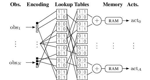
In this work, we challenge the necessity of relying on weightbased neural networks, i.e., those that rely on large matrix multiplications during inference, for learning continuous control policies. Instead, we introduce DWCs (Differentiable Weightless Controllers), a symbolic-differentiable architecture for continuous control in which dense matrix multiplication is replaced with sparse boolean logic. Figure 1 illustrates the inference pipeline.

At their core lie differentiable weightless networks (DWNs) (Bacellar et al., 2024), an FPGA-compatible and alternative variant of logic-gate networks (LGNs) (Petersen et al., 2022) that were originally proposed for highthroughput, low-energy classification tasks. We extend the DWN architecture to the continuous RL domain, enabling synthesis of control policies that are digital circuits instead of real-valued functions. Specifically, we introduce a dataadaptive input encoding that converts real-valued input signals into binary vectors, and a trainable output decoding that converts binary output vectors into real-valued actions of suitable range and scale. The resulting DWCs are compatible with gradient-based RL, and we demonstrate experimentally that the learned DWCs match weight-based neural network baselines (full precision or quantized) on standard MuJoCo benchmarks, including the high-dimensional Humanoid task.

At deployment time, DWCs process continuous observations by quantizing them using quantile binning and thermometer encoding, resulting in a fixed-width bitvector representation for each observation dimension. The bitvectors are concatenated and processed by a DWN, which consists of sparsely-connected layers of boolean-output lookup tables (LUTs) (Bacellar et al., 2024). The final layer produces a fixed number of bit outputs per action dimension. These are summed using a popcount operation and converted to a final action value using a single-cycle (SRAM) memory lookup.

As a consequence, DWCs are compatible with embedded hardware platforms, especially FPGA platforms that explicitly support LUT operations. Here, DWCs can run with fewor even single-cycle latency and minuscule (e.g. Nanojoulelevel) energy per operation, as we demonstrate for the case of an AMD Xilinx Artix-7.

Besides their efficiency, DWCs also have high potential for interpretability, because they cconsist of sparse, discrete, and symbolic elements instead of dense, continuous, matrix-multiplications in standard networks. For instance, the sparse connectivity in the first layer allows for direct identification of the input dimensions and thresholds utilized by the controller.

Contributions. To summarize, our main contribution is the symbolic-differentiable DWC architecture that extends previous DWNs from classification to continuous control tasks. We demonstrate that • DWCs can be trained successfully using standard RL algorithms, reaching parity with floating-point policies (full precision or quantized) in most of our experiments.

• DWCs are orders of magnitude more efficient than previously proposed architectures, achieving few-or even single-clock-cycle latency and nanojoule-level energy cost per action when compile to FPGA hardware.

• DWCs allow for straightforward interpretation of some aspects of the policies they implement, specifically which input dimensions matter for the decisions, and what the relevant thresholds are.

We briefly review deep reinforcement learning for continuous control, and provide background details on DWNs.

Reinforcement learning studies how an agent can learn, through trial and error, to maximize return (cumulative reward) while interacting with an environment (Sutton & Barto, 2018). There exist various reinforcement learning algorithms that are compatible with our setting of continuous control (continuous actions and observations). In the main body of this work we investigate the performance of DWCs with the state-of-the-art Soft-Actor Critic (SAC) method (Haarnoja et al., 2018). Results for Deep Deterministic Policy Gradient (DDPG) (Lillicrap et al., 2016) and Proximal Policy Optimization (PPO) (Schulman et al., 2017) can be found in Appendix B.

SAC is an off-policy method, which keeps a buffer of previous state transitions and taken actions. It updates the parameters of the policy network based on this buffer with advantage estimations from two auxiliary networks (called critics). Actions during training are sampled stochastically from a normal distribution, parametrized as N (µ θ , σ θ ), with θ being learned parameters. During deployment, the mean action is used deterministically.

Weightless networks (Aleksander, 1983;Ludermir & de Oliveira, 1994) Thermometer encoding. DWNs operate on binary signals, so any real-valued observation has to be discretized. For any input x ∈ R and predefined thresholds τ 1 < • • • < τ B , define the thermometer encoding (Carneiro et al., 2015), Logic Layers. A DWN with L layers comprises binary activation maps b (ℓ) ∈ {0, 1} D ℓ , ℓ = 0, . . . , L. Where D 0 is the size of the encoded input, and for ℓ > 0, D ℓ denotes the number of LUTs in layer ℓ. Each LUT is a boolean function with arity k. For LUT i we form an address

They are learned via straight-through estimation during training, as described in Bacellar et al. (2024). While Bacellar et al. (2024) only train the first layers interconnect, we also make the later ones learnable. This is inspired by results in Kresse et al. (2025b), where training accuracy consistently improves if later-layer interconnects are learnable. Each LUT stores a table, T , of 2 k binary values. The output bit is the addressed entry, where addr(•) maps the k-bit vector to its integer index. Concatenating all output bits yields b (ℓ+1) .

Group aggregation. To allow for multi-dimensional outputs, the final binary features b (L) of a DWN are partitioned into disjoint groups. For a group G, a group sum is computed,

with a temperature τ > 0 used as a scale during training.

For classification, these s G serve as logits for a softmax; at inference, the operation reduces to efficient popcount and argmax operations.

Gradient surrogate. Because the forward pass is discrete, DWNs rely on surrogate gradients for training. We follow Bacellar et al. (2024), who propose an extended finitedifference (EFD) estimator that perturbs the LUT address and aggregates contributions from all possible addresses with weights proportional to their Hamming distances.

We now provide details on how DWCs extend DWNs to continuous control tasks. In terms of architecture, we adapt the input quantization, such that it can deal with changing input distributions during training, and we adapt the output layer to allow for multi-dimensional continuous actions. Subsequently, we describe the RL training procedure.

We map observations to binary inputs via clipped normalization and thermometer encoding. For each dimension j, we normalize with running mean and standard deviation, subsequently clipping: xj = clip (x jµ j )/σ j , -10, 10 . While in deep RL, normalization is often considered optional, we employ it always, as we are projecting from R to a restricted, a priori known interval, for which we can subsequently choose thermometer thresholds E j . After normalization, we employ the same thermometer thresholds for all dimensions d in .

Using an odd number of bits B, we place thresholds at stretched-Gaussian quantiles: let q m = m/B for m = 1, . . . B -1 and an additional quantile at 1 2 , and set a stretch factor

, where Φ -1 is the inverse cumulative probability distribution of the standard Gaussian. Define τ j,m = s Φ -1 (q m ) for m = 1, . . . , B so that the first/last thresholds land exactly at ±10, and the additional threshold at 0. The thermometer code is 0) for the first DWN layer. Figure 2 illustrates the resulting input thresholds.

To produce continuous actions we reinterpret the group aggregation as a bank of scalar heads, one per action dimension. Let {G 1 , . . . , G dact } be a partition of the final bits b (L) .

For dimension d we first normalise the group sum:

We then apply a per-dimension affine transformation:

with learnable scales α d > 0 and bias β d ∈ R. To ensure positive α d , we parameterize α d = e α d,p . This head is fully differentiable and integrates with policy-gradient objectives. The emitted l d is the generated logit, which is passed through an additional tanh in the case of SAC before computing the final action. The initialization value of α d restricts the initial policy actions to a subinterval of the possible action space. This is comparable to initializing the final layer parameters with a low standard deviation, a strategy that has been shown to improve learning in RL (Andrychowicz et al., 2020).

At deployment, the initial threshold operations required for the thermometer encoding should be implemented in a platform-dependent way. Commonly, actual sensor readings are obtained as integers from an analog-to-digital converter (ADC), in which the initial bitvector b (0) can be computed as fixed integer-to-thermometer lookup per sensor channel (the constants used for normalization and clipping are fixed after training, so they can be folded into the threshold values).

Subsequently, actions can be computed using only LUT evaluations, popcounts and SRAM memory lookups: starting with b (0) , the bitvectors propagate through L LUT layers to produce b (L) . For each action head d, we popcount its group G d to obtain the integer s G d . An SRAM then implements the mapping from this popcount to the emitted control word, i.e., s

and, e.g. for SAC, the subsequent tanh. In practice, the table would output an integer actuator command. Note that, unlike the standard DWN classification head, no temperature parameter τ is required, simplifying hyperparameter tuning.

The learnable components of DWCs are the LUT entries, their connectivity, and the mapping from popcounts to action values. The latter are parameterized as an affine transformation, potentially followed by an additional hyperbolic tangent, so standard gradient-based learning is applicable.

To learn the former two in a differentiable way, we rely on the connection learning and the extended finite difference surrogate gradients of Bacellar et al. (2024), making DWCs overall compatible with any gradient-based reinforcement learning algorithm.

Note that, similar to previous work on quantized neural networks (Kresse & Lampert, 2025), during RL training we only parametrize the policy networks as DWCs, because only these are required at deployment time. All auxiliary networks, such as the critic networks and the σ θ head for SAC can remain as standard floating-point networks.

We evaluate the proposed Differentiable Weightless Controllers on five MuJoCo tasks (Todorov et al., 2012): Ant-v4, HalfCheetah-v4, Hopper-v4, Humanoid-v4 and Walker2d-v4, using SAC for training. We also investigate returns for DDPG and PPO in Appendix B.

Baselines. As baselines, we use two weight-based neural network setups: First, we use full-precision (FP) models trained with the CleanRL implementation (Huang et al., 2022) of SAC, as reported in Kresse & Lampert (2025).

Here, the network has 256 neurons in the hidden layer. In contrast to the original CleanRL implementation, the networks use running input normalization, as this has been found to improve return for SAC for our tasks. Second, we compare against the QAT-trained low-precision models (2or 3-bit weights and activations) from Kresse & Lampert (2025), which were designed to match the FP baselines at more compact network sizes.

DWC. We adopt the same architectures as in the baseline implementations, except that we use DWCs for the policy networks. Unless stated otherwise, DWCs are instantiated with two layers of k=6 input LUTs. We employ 1024 LUTs 0 0.5M 1M 0 2,000 4,000 6,000 per layer, padding the last layer with LUTs to be divisible by the action dimension. Observations are discretized to 63 thermometer thresholds per dimension, as described in Section 3. Ablation studies on these choices are available in Section 5.

Hyperparameters. We adopt the protocol used in CleanRL, hence we use the same hyperparameters across each algorithm for all investigated tasks. For training the DWCs we use the same hyperparameters as for the baselines, as specified in Appendix C.

Training and Evaluation. For each configuration, we train 10 models with different random seeds. Each model is trained for 1 million environment steps and then its undiscounted return is estimated from 1000 rollouts of the fixed policy from random starting states. Compared to the default CleanRL implementation, we perform all evaluation rollouts without exploration noise.

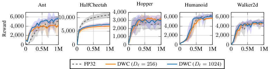
Figure 3 shows the training dynamics of DWCs versus the FP baseline. Table 1 shows the resulting returns after training, also including results for quantized networks. Clearly, DWCs learn policies of comparable quality to the floating point networks, and hence they can readily serve as more drop-in replacements, from a reward perspective. An exception is the HalfCheetah environment, where we observe a substantial return gap. Note that models with a cumulative reward of 7.5k on HalfCheetah are not performing badly at all, indeed they learn to run, i.e. master the environment. However, they do so at a slower pace than, e.g., the FP models with 11.5k reward.

Our findings confirm the observation from Kresse & Lampert (2025) that HalfCheetah is the task most resistant to network reduction and quantization, presumably because the task is capacity-limited. We study this phenomenon further in Section 5 and the Appendix.

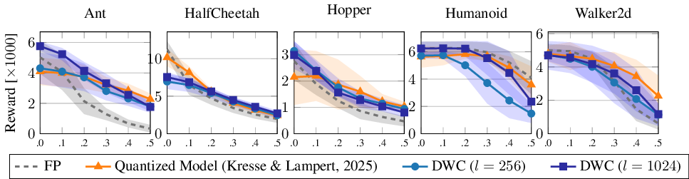
Following Duan et al. (2016), we also assess the robustness of DWCs to observation noise. We inject zero-mean Gaussian noise with standard deviations σ ∈ {0.1, 0.2, 0.3, 0.4, 0.5} into normalized observations (unit variance) and compare DWCs to the FP baseline and the quantized noise robustness results from Kresse & Lampert (2025). Figure 5 reports the results, which show that DWCs achieve noise robustness profiles comparable to that of the quantized network, and generally on the same level as or even better than floating point networks. The only exceptions are the compact (D ℓ = 256) models, which perform worse on Humanoid under high noise.

The main advantage of DWCs over standard deep controllers is that they consist exclusively of elements that have direct representations on low-energy hardware platforms. To demonstrate this, we perform synthesis and implementation (place-and-route) of the resulting networks for an FPGA, reporting required resources and energy estimates based on the manufacturer-provided tools.

We run out-of-context (OOC) synthesis and implementation with the AMD Vivado toolchain (2022.2), targeting an AMD Xilinx Artix-7 XC7A15T (speed grade -1), see Table 10 in Appendix F for the available device resources. Note that the selected FPGA only has a total of 10,400 LUT-6s and twice this amount of flip-flops (FFs), which is a much smaller FPGA than previous investigations of DWNs (Bacellar et al., 2024). Instead, our setup is directly comparable to Kresse & Lampert (2025), who used the same reference FPGA platform and tool chain.

We target a clock frequency of 100 MHz, inserting up to two pipeline stages-the first one between the two LUT layers, and the second one before the popcount-until we meet the desired timing. As our design is implemented OOC we do not consider any overhead due to I/O interfaces. Furthermore, we assume that all observation normalization steps and the final BRAM lookup for the action scaling take place outside of the FPGA, because these depend on the specific application (e.g. the input format depends on the type of ADCs, the output format on the type of DACs).

Table 2 reports Reward, LUTs, FFs, BRAMs (B), Latency (Lat), Power (P), Throughput (TP), and Energy per Action (E.p.A) for each setup. Since full precision policies are not practical on the selected hardware, we compare to the quantized networks from Kresse & Lampert (2025). The only difference to their setup is that our values for power estimation are based on the toolchain’s post-implementation power report, rather than the less accurate Vivado Power Estimator.

The results show that DWCs exhibit orders of magnitude lower latency and energy per action compared to the lowbitwidth quantized networks. For our standard D ℓ = 1024 setup, latency is only 2 or 3 clock cycles, the throughput is the maximal possible of 10 8 actions per second, and the energy usage is in the range of 2 Nanojoule per action. In contrast, Kresse & Lampert (2025) reports orders of magnitude higher and much more heterogeneous resource usage: their latencies range from 21 cycles to over 162,000 cycles, their throughput between 4.1 × 10 3 and 4.8 × 10 6 actions per second, and their energy usage per action between 2.8 × 10 -5 and 6.5 × 10 -8 Joule.

Additionally, in contrast to the quantized models, the computational core of DWCs does not require any BRAM or DSP resources, making them deployable on even more limited hardware than the already small FPGA investigated here.

To illustrate the scaling behavior, we include results for even smaller DWCs with layer width D ℓ = 256 in Table 2. This results in single-clock-cycle latency, still maximum throughput, and energy usage per action reduced further by a factor of approximately 2.

In this section we report ablation studies on the scaling behavior of DWCs with respect to their layer widths and the input size to the LUTs. Subsequently, we demonstrate how the sparse binary nature of DWCs allows for insights into their learned policies.

We first investigate the effect of different network capacities.

Concretely, we study the effect of varying the layer sizes (widths) and the number of inputs to each LUT. Further ablations on the impact of input resolution and number of layers are available in Appendix E.

Layer Width. Assuming that the number of layers is fixed, a large impact on the network capacity comes from the layer width, D ℓ , i.e. the number of LUTs. We run experiments in the previous setting with layer width varying across {128, 256, 512, 1024, 2048, 4096}, where the last layer is padded to be divisible by the action dimension, and report the results in Figure 4. For four of the tasks, the quality is relatively stable with respect to layer widths, with per-layer sizes above 256 generally exhibiting returns similar to the floating-point baseline. This indicates that these learning tasks are not capacity limited, but that at the same time no overfitting effects seem to emerge. As previously observed, HalfCheetah is an exception, where we observe that the quality of the policy increases monotonically with the width of the layers. There are two possible explanations for this phenomenon observed on HalfCheetah: 1) smoother actions, due to a higher output layer width, resulting in more possible actions, as each action head has a resolution of the size of the partition G d ; and 2) higher representation capacity and input layer resolution, as more LUTs can connect to different bits in the first layer. In light of the results in Kresse & Lampert (2025) that a 3-bit resolution suffices for HalfCheetah in the output actions; and hidden capacity appears to be the major bottleneck in quantized neural networks, we hypothesize that 2) is the case.

To explore this further, we investigate a significantly larger DWC with D ℓ = 16, 384 LUTs per layer and inputs quantized to 255 levels (instead of 63). Due to the larger layer size, we do not train the second layer interconnect, but initialize it randomly and keep it fixed; the remaining training setup remains unchanged. Results are depicted in Figure 4 (dashed light gray entry). With a median return value above 10.3k, this setup now matches the returns of the quantized baseline (median return 10.4k) and falls within the region of uncertainty of the floating-point policy (median return 11.5k). Notably, even at the increased layer width, DWCs requires only 32k lookups (and six popcounts, in the case of HalfCheetah)-substantially fewer than 70k+ multiplyaccumulate operations by the two baselines. We take this result as evidence that DWNs can scale to such tasks, if required.

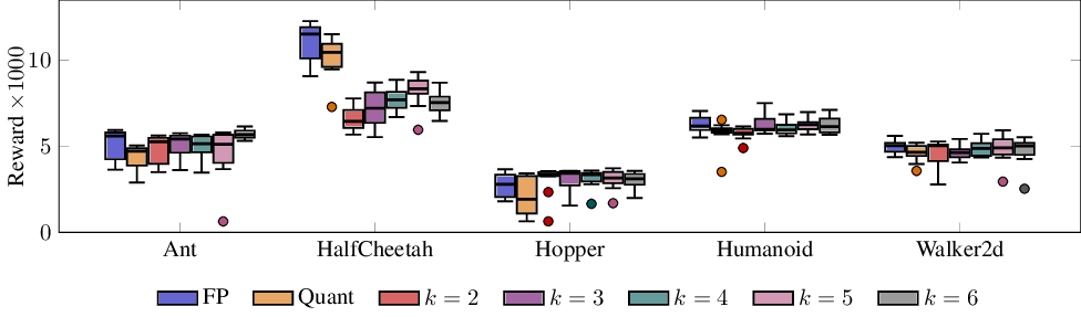
LUT Size Besides the number of LUTs, also the number of inputs per LUT, k, impacts the network capacity, as more inputs imply that layers are more densely connected, and that the LUTs themselves can express more complex relations.

In Figure 8 in the appendix, we report average returns for all tasks with k varied from {2, 3, 4, 5, 6} and constant layer width D ℓ = 1024. In line with the previous experiments, we observe capacity effects limiting returns only for HalfCheetah, while the other returns remain largely unaffected. This suggests that in practice, the number of LUT inputs can be chosen based on what matches the available hardware. For FPGAs, built-in support for k = 6 is common, whereas on custom ASICs, any k larger than 2 could be prohibitively expensive.

Deep networks are often criticized as black boxes (Molnar, 2020;Vouros, 2022), where the trained policy offers little insight into which feature values drive specific actions.

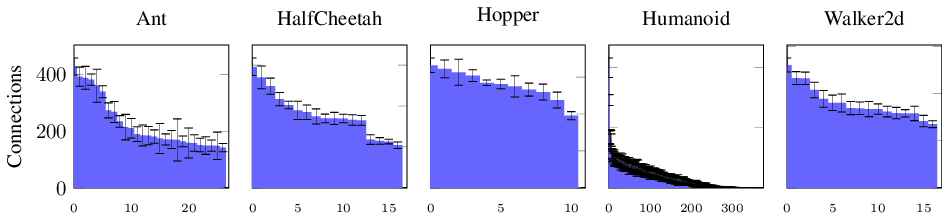
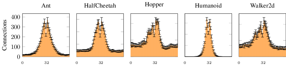
Here, we demonstrate how binary sparse DWCs can potentially contribute to overcoming this issue to some extent. Because input bits correspond to specific input thresholds and connections to processing LUTs are both sparse and learned, we can infer feature importance simply by counting outgoing connections. Figure 6 illustrates the number of connections received per observation dimension, averaged over the ten trained models (D ℓ = 1024). The entries are sorted after aggregation according to the mean number of connections. The data shows that connectivity is nonuniform: some input dimensions receive substantially more connections than others, especially for higher-dimensional observation tasks, i.e. Ant and Humanoid. The low standard deviations across independent models indicate that the network consistently identifies the same specific dimensions as relevant for solving the task.

Interestingly, for Humanoid, a large number of observation dimensions receive no connections at all (on average 275 out of 376 receive a connection). Because the trained model nevertheless attains performance comparable to the FP model, we conclude that the unconnected dimensions are not necessary for good control. In contrast, torso velocity observations receive the highest number of connections for Humanoid. As the reward function is heavily dependent on forward velocity, this suggests the DWC has identified the features most directly correlated with the reward signal.

Figure 7 shows the distribution of connections across input threshold bits, averaged over dimensions and over trained models. Recall that the input bit with index 31 out of 63 corresponds to the normalized observation value of 0, index 0 corresponds to the normalized value of -10 and index 63 to 10 (Section 3).

Perhaps unsurprisingly, the highest connectivity density is typically found around the normalized observation value of zero. However, instead of a Normal distribution, we observe two distinct modes left and right of the center. This is potentially explained by the reduced probability density captured by the 0 threshold, which is artificially inserted between the two thresholds to its left and right. Furthermore, some tasks (Hopper, Walker, and HalfCheetah) show heavier tails than the others (Ant, Humanoid). We hypothesize that the heavier tails are explainable by the lower observation dimensionality of their respective tasks, and not due to an increased importance of extreme observation values. This hypothesis is supported by Figure 11 in Appendix E, showing the same plot for DWCs with D ℓ = 128, which generally exhibit similar return performance (see Figure 4). Here, the tails are lighter, with the maximal number of possible first-layer connections having been significantly reduced to just k × D ℓ = 768, indicating that the heavier tails observed for the larger models are indeed due to the higher number of possible connections, suggesting that many connections might not be contributing significantly.

In

Table 4 and Table 5 show SAC and DDPG hyperparameters, respectively. Table 6 shows the PPO floating-point hyperparameters used in our experiments, while Table 7 shows the PPO hyperparameters used for DWCs.

Major differences between FP and DWCs PPO hyperparameters are a ×10 learning rate for DWCs, a lower entropy coefficient, and a lower max gradient norm. The initial log α is conceptually similar to the floating-point std parameter, which corresponds to the initialization of the policy network’s output variance.

Tables 8 shows the search space for the PPO hyperparameter tuning for DWCs, while Table 9 shows the search space for the PPO hyperparameter tuning for the FP baseline. Remaining hyperparameters were set to the values in Table 6, which correspond to CleanRL (Huang et al., 2022) defaults. Hyperparameter tuning was performed jointly across Ant, Hopper, Walker, and HalfCheetah, optimizing for return after 1M timesteps over 3 seeds. Hyperparameter search was performed with Optuna (Akiba et al., 2019) using the Tree-Structured Parzen Estimator with 100 trials. The hyperparameter search for DWCs took 25 days of compute, which we distributed over 10 GPUs.

Figure 8 shows an ablation over the LUT input size k from 2 to 6 inputs. Larger k increases the expressivity of each LUT, but also exponentially increases the number of parameters per layer.

Clearly, already k = 2 achieves good results across all tasks, being comparable for all except for HalfCheetah. For LGN 1

LGN 2

LGN 3

-synthesis resource utilization for one synthesized model, BRAM (B), end-to-end latency (Lat) in microseconds, power estimated by the Xilinx Power Estimator (P) in Watts, peak throughput (TP) in actions per second, and energy per action (E.p.A.) in Joule on a Artix-7 XC7A15T-1 at 100 MHz. Shown reward is the median over all ten models.