Accelerated Execution of Bayesian Neural Networks using a Single Probabilistic Forward Pass and Code Generation

While DNNs are among the most effective methods for learning and predicting under uncertainty, they fundamentally lack the ability to quantify any uncertainty in a principled, mathematical manner. In classification tasks, for example, the softmax function is commonly used to produce class-wise output scores that are interpreted as probabilities. However, these softmax-derived values do not possess a rigorous probabilistic interpretation; they are best understood as confidence scores without a theoretical foundation grounded in probability theory. This limitation becomes particularly apparent when models are exposed to data samples that differ significantly from the training distribution. These are commonly referred to as out-of-domain (OOD) data. In such cases, neural networks often produce highly confident yet incorrect predictions, without any mechanism to signal elevated uncertainty or to indicate that the input lies outside the model’s domain of competence.

A theoretical framework to allow neural architectures to say “I don’t know” is cast by Bayesian statistics, resulting in a class of probabilistic models called Bayesian neural networks (BNNs). They provide predictions in the form of a formal probability distribution, in which, in an simple setting, the mean would correspond to the prediction itself while the uncertainty is coded as variance or standard deviation of this distribution.

BNNs, while providing a mathematically rigorous framework for uncertainty estimation, incur an even greater computational burden than standard DNNs, which are already exceedingly expensive in both training and inference.

Their high computational cost for predictions arises from the need to sample weights from posterior distributions and perform multiple forward passes to estimate predictive uncertainty. These repeated sampling and forward pass operations during prediction significantly increase latency, posing challenges for deploying BNNs in resource-constrained environments such as Internet of Things (IoT) devices and embedded systems.

In general, probabilistic modeling has gained significant interest within the ML community, leading to extensive related work [22,42]. However, relatively little research addresses probabilistic modeling from a hardware perspective.

Notable exceptions exist regarding hardware-efficient probabilistic circuits [37,57]. Furthermore, a hardware-aware cost metric for probabilistic models has been introduced within tractable learning [21]. Specialized hardware accelerators for BNNs employing numerous on-chip pseudo-random number generators have also been proposed [9,11,54].

Probabilistic inference based on BNNs is a problem of exceptional complexity due to the inherent complexity of random variable algebra. At the same time, uncertainty is of high importance when bringing ML models into the “wild”, where sensors are hindered by noise, occlusions, and previously unseen settings. 1 To successfully deploy BNNs on resource-constrained devices requires to combine multiple methods to bridge the gap among BNN requirements on memory and compute and the corresponding hardware capabilities.

One approach to mitigate this challenge is using partially Bayesian neural networks, treating only a subset of weights probabilistically [52]. This significantly reduces training complexity compared to full Bayesian models. Determining the appropriate number of probabilistic parameters remains an open question, as excessive reduction can degrade predictive performance. Moreover, partial BNNs typically still require multiple forward passes for uncertainty estimation, limiting efficiency on resource-constrained devices. In contrast, last-layer methods avoid multiple forward passes by encoding probabilistic samples into multi-headed architectures [53]. Steger et al. demonstrates that a function-space-based repulsive loss effectively enables probabilistic inference even for pretrained models by only training an ensemble of probabilistic output layers [53].

A widely used approach to enable probabilistic reasoning in neural networks is Stochastic Variational Inference (SVI), which approximates the posterior distribution of weights by assuming a parameterized family of distributions [42], typically Gaussians. While SVI provides a tractable framework for Bayesian inference and is more efficient and GPUfriendly compared to Markov Chain Monte Carlo (MCMC) due to its reliance on gradient-based optimization and backpropagation, it still incurs substantial computational costs from weight sampling and the need for multiple forward passes [28]. An alternative solution is to adopt an analytical approximation, such as the Probabilistic Forward Pass (PFP) [47], which represents an extreme case of simplification by assuming not only Gaussian-distributed weights but also Gaussian-distributed activations. This approximation enables a closed-form solution for uncertainty estimation.

While still treating all weights in a probabilistic manner, PFP requires only a single, albeit more complex, forward pass for both prediction and uncertainty estimation, eliminating the need for weight sampling and multiple forward passes.

Uncertainty in probabilistic machine learning is categorized as either aleatoric or epistemic [29]. Aleatoric uncertainty originates from inherent noise in the data and is irreducible, while epistemic uncertainty reflects model uncertainty due to limited knowledge and can be reduced with more data or better modeling. For classification problems, aleatoric uncertainty is typically quantified using Softmax Entropy (SME), while epistemic uncertainty-including out-ofdistribution (OOD) samples-is measured using Mutual Information (MI). We refer to Section 2.3 for a detailed discussion.

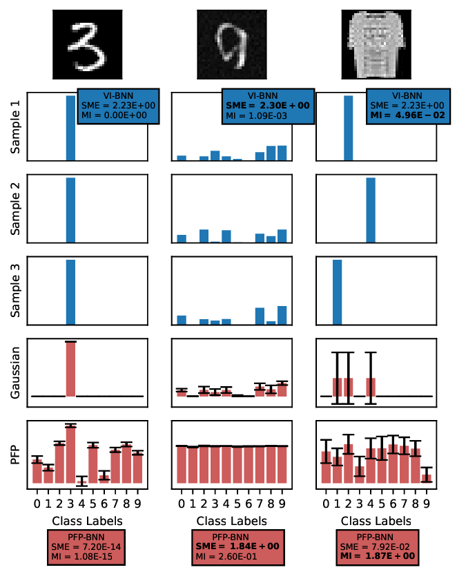
Figure 1a illustrates the performance of a SVI-based BNN on images from three representative datasets. The training dataset MNIST [36] represents in-domain data, while Ambiguous-MNIST [41] introduces aleatoric uncertainty through samples between classes, and Fashion-MNIST [56] contains OOD images of fashion items. In the following, we will refer to these datasets in combination as “Dirty MNIST”. Aleatoric uncertainty, quantified via SME, appears for ambiguous samples seen within one sample between classes; OOD images trigger confident but mutually disagreeing predictions.

For each SVI sample, the raw unnormalized outputs, called logits, are typically normalized using a softmax function, and the most likely class is predicted by selecting the maximum value. Disagreement across predictions, quantified by MI, signals epistemic uncertainty, indicating potential OOD data.

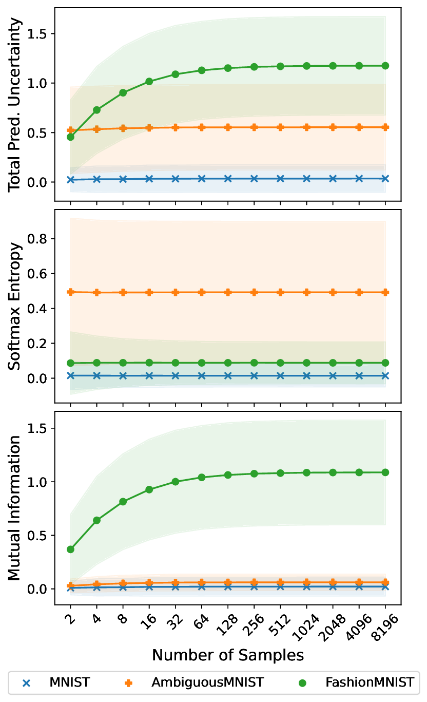
Figure 1b demonstrates that reliable uncertainty quantification requires many samples, causing significant computational demands in traditional BNNs. For illustrative purposes, only three samples are shown in Figure 1a. The Figure also includes a Gaussian approximation that summarizes the logit samples using their mean and standard deviation.

While this approach somewhat obscures detailed aleatoric and epistemic distinctions, it offers significant compactness benefits. PFP consistently utilizes this strategy through a single distribution-propagating forward pass. In practice, it effectively predicts and distinguishes both uncertainty types. However, since PFP uses non-standard probabilistic operators, an efficient hardware-specific implementation of these operators is required before the method can be used in practice. These custom operators can be implemented using deep learning compilers, such as TVM [13], which enable automatic code generation and performance tuning [51]. By leveraging these tools, the rather complex operations of the Probabilistic Forward Pass can be optimized for specific hardware architectures, allowing BNNs to run more efficiently in resource-limited environments while maintaining robust uncertainty estimation.

In detail, this work makes the following contributions: showcasing MNIST [36] and Ambiguous-MNIST [41] as in-domain examples, and Fashion-MNIST [56] as an out-of-domain sample. Variability in class predictions demonstrates aleatoric uncertainty (higher Softmax Entropy, SME), whereas variability across predictive samples indicates epistemic uncertainty (higher Mutual Information, MI). SVI and PFP effectively quantify these uncertainties. Note: Only three SVI samples shown, insufficient for robust estimation. (b) Influence of predictive sample count on uncertainty metrics. Softmax Entropy (aleatoric uncertainty) remains stable, while Total Predictive Uncertainty and Mutual Information (epistemic uncertainty), especially for out-of-domain data (Fashion-MNIST), require more samples for reliable OOD detection.

• We propose a training pipeline based on Stochastic Variational Inference and demonstrate that the Probabilistic Forward Pass achieves comparable performance in uncertainty estimation and out-of-domain detection, validated on the “Dirty MNIST” dataset.

• We extend the deep learning compiler TVM by integrating essential probabilistic operators for multi-layer perceptron (MLP) and convolutional neural network (CNN) architectures, enabling the efficient execution of PFP-based models on ARM processors.

• We implement optimized execution schedules as well as manual and automatic tuning strategies for computationally intensive PFP operators, ensuring high performance on resource-constrained ARM CPUs.

• We evaluate the practical feasibility of our approach through benchmarks on embedded ARM processors, demonstrating significant performance improvements that facilitate the deployment of BNNs for uncertaintyaware edge and IoT applications.

As we will see, although the PFP concept relies on highly non-standard operators, casting the problem within a mapping framework such as TVM enables deployment without specialized libraries while also allowing performance optimizations with reasonable effort. In more detail, we address the following research questions and aim to provide corresponding answers in what follows:

(1) How good is the quality of PFP-based Bayesian neural architectures?

(2) How well does TVM support custom operator implementation?

(3) How fast is the PFP approach, when employing various optimization techniques, compared to a SVI-based BNN?

The remainder of this paper is structured as follows. Section 2 reviews related work on efficient BNN implementations and their deployment on resource-constrained devices. Section 3 presents the theoretical foundation and Section 4 training, and uncertainty evaluation of PFP. Section 5 discusses the implementation of custom operators using TVM, highlighting the specific challenges associated with PFP operators. Section 6 covers operator tuning, profiling, and benchmarking, comparing PFP-and SVI-based BNNs on embedded ARM processors. Finally, Section 7 summarizes the key findings and conclusions of this work. The presented PFP operator library is publicly available. 2

This section provides a brief introduction to BNN methods, with a particular focus on related work concerning efficient BNN inference. We further clarify the distinction between different types of uncertainty and review methods for efficient inference on resource-constrained embedded systems, specifically in the context of BNNs.

Bayesian neural networks integrate Bayesian inference (BI) into neural networks by treating weights as random variables rather than fixed values [43]. Weights are sampled from distributions, enabling uncertainty estimation and improved generalization, particularly in data-scarce or noisy settings. BNNs place a prior distribution over the network’s weights, and then, given observed data, compute a posterior distribution. The prior reflects any previous knowledge about the weight values, while the posterior captures the updated beliefs after seeing the data [28,42]. This probabilistic framework quantifies predictive uncertainty, making BNNs valuable for uncertainty-sensitive and safety-critical tasks.

In BNNs, weight distributions can take various forms, but Gaussian approximations are common due to their mathematical properties and computational efficiency. Computing the posterior distribution of weights is in general analytically intractable due to the high-dimensional and non-convex nature of neural networks [28]. Training and prediction involve sampling weights from these distributions, unlike deterministic networks that use fixed point estimates. This sampling enables BNNs to produce a distribution of possible outcomes rather than a single prediction.

Such distributions facilitate uncertainty estimation and can help detect out-of-domain data.

The equivalent of training in this context is performing Bayesian inference to learn this weight distribution [28]. BI techniques are commonly categorized into two classes: sampling-based methods and variational methods that optimize an approximate posterior distribution. Markov Chain Monte Carlo (MCMC) methods, for instance, sample directly from the posterior distribution, making them particularly well-suited for BNNs [8]. These methods construct a Markov chain with the target posterior as its equilibrium distribution. Hamiltonian Monte Carlo (HMC) [44] in combination with the No-U-Turn-Sampler (NUTS) [26] is considered the gold standard in terms of quality and reliability. Although offering strong theoretical guarantees, MCMC methods suffer from high computational costs due to slow convergence in high-dimensional spaces and the requirement for a large number of samples.

Variational Inference (VI) reformulates BI as an optimization problem, improving scalability for large datasets and models [5,25] While MCMC offers a theoretically sound approach for posterior estimation but is computationally expensive and difficult to scale, SVI offers a more practical alternative, trading off accuracy for improved scalability and faster convergence, making it a popular choice for BNNs in modern deep learning applications.

Bayesian Neural Networks and Efficient Inference. Over the years, a wide range of methodologies for BNNs has been developed; for a comprehensive survey, we refer to [28,42]. In the following, we highlight some of the most pioneering works that focus on approximate inference techniques designed to enable efficient prediction with BNNs. While SVI and MCMC methods are mathematically grounded many alternative approaches only loosely relate to these foundational principles. This often enables improved computational efficiency, but comes at the cost of reduced theoretical rigor and degraded uncertainty estimation performance.

To reduce computational cost, Blundell et al. proposed an SVI-based approach that approximates the posterior using a simplified distribution [6]. This approach reduces computational costs compared to MCMC but remains challenging for deployment on resource-constrained platforms such as mobile devices. Gal and Ghahramani advanced BNN efficiency by proposing Monte Carlo Dropout [19,20], which approximates BNNs by applying dropout at inference. This method provides uncertainty estimates with minimal computational overhead, interpreting dropout as a probabilistic mechanism, making it well-suited for constrained environments. However, its approximation quality varies notably.

Deep Ensembles (DE) are another prominent example in this category of algorithms. They provide uncertainty estimates by training multiple independent neural networks and aggregating their predictions [34]. Due to their simplicity and effectiveness they are widely used. A fundamental limitation shared with MCMC methods is the substantial memory overhead at inference time, as both approaches require maintaining multiple sets of model parameters or posterior samples, making them impractical for deployment on resource-constrained embedded devices.

Repulsive ensembles [15] extend Deep Ensembles by promoting diversity among ensemble members. Steger et al. [53] show that a function-space repulsive loss enables probabilistic inference even for pretrained models by training only an ensemble of probabilistic output layers.

Overall MCDO and ensemble methods have all improved efficient Bayesian inference significantly. However, as a common theme they all discard the formal theoretical foundations, found in SVI and MCMC methods. While these foundational works have advanced efficient Bayesian inference, direct applications to mobile processors remain limited. Accelerated Execution of Bayesian Neural Networks using a Single Probabilistic Forward Pass and Code Generation7

In the probabilistic ML context uncertainty is categorized into aleatoric and epistemic uncertainty [29]. Aleatoric uncertainty stems from inherent noise in the data, making it irreducible even with unlimited data. It arises when input features contain measurement noise or the output variable is intrinsically unpredictable. Aleatoric uncertainty can be homoscedastic (constant across inputs) or heteroscedastic (input-dependent).

Epistemic uncertainty arises from a lack of knowledge, such as missing data or suboptimal models. It is reducible and decreases with more data or model refinement. This uncertainty is prominent in underrepresented input regions, including OOD data. The key distinction is that aleatoric uncertainty is data-driven and irreducible, while epistemic uncertainty is model-related and can be reduced.

BNNs distinguish between aleatoric and epistemic uncertainty in both regression and classification tasks. In regression, aleatoric uncertainty is modeled via a heteroscedastic head that predicts data-dependent noise. For classification, aleatoric and epistemic uncertainty are commonly estimated via Softmax Entropy and Mutual Information, respectively [41].

Both MCMC and SVI require sampling from the posterior weight distribution. If 𝑁 predictive samples are needed, 𝑁 complete weight sets must be drawn, and 𝑁 forward passes executed. As shown in Figure 1a, each predictive sample in classification yields distinct predicted logits. For classification, total predictive uncertainty is quantified using Shannon Entropy [50]:

Here 𝑝 (𝑦 = 𝑐 |𝑥, 𝑤 𝑛 ) denotes the probability of prediction 𝑦 and ground-truth class 𝑐 being identical, given input 𝑥 and weight sample 𝑤 𝑛 from the 𝑛-th sample. D denotes the full dataset, 𝐾 the number of classes, and 𝑁 the number of samples. This total predictive uncertainty is decomposed into their aleatoric and epistemic components, measured by the Softmax Entropy,

and Mutual Information [14]

For the Shannon Entropy the samples are summed first, while the Softmax Entropy sums first over classes 𝐾, and thereby encodes the mean of the aleatoric uncertainty.

Resource-efficient uncertainty estimation in neural networks, particularly BNNs, has become an increasingly important area of research, especially given the growing demand for deploying sophisticated machine learning models on resource-constrained devices such as mobile processors.

Resource-Efficient Deployment on Mobile Devices. Deploying machine learning models on mobile processors requires careful optimization for computational and memory constraints. Chen et al. introduced TVM [13], an automated deep learning compiler that optimizes models for diverse hardware backends, including mobile ARM processors. TVM facilitates efficient deployment of deep neural architectures by automating optimizations and supporting hardwarespecific enhancements such as quantization and model pruning.

Quantization [27] reduces the precision of neural network weights and activations, significantly lowering inference resource requirements. Deep compression methods, including pruning and quantization [23,49], reduce the resource footprint, enhancing applicability to mobile processors. Neural architecture search and automatic compression, combined with reinforcement learning [10,12,24,32], automate architecture refinement and compression parameter selection, optimizing bit width and sparsity, and enabling compression at the layer, channel, or block level. For a more detailed overview of resource-efficient neural network inference on embedded systems, including a comparison of various compression methods and hardware architectures, we refer to [48].

Considering the intersection of Bayesian methods and neural networks from a different perspective, Louizos et al.

propose Bayesian compression techniques for DNNs [40], leveraging priors to guide pruning while using posterior uncertainties to determine optimal fixed-point precision. Although relevant for mobile DNN deployments, this approach does not address the efficiency of BNNs.

Bayesian Neural Networks on Resource-Constrained Devices. Although direct research on deploying BNNs on mobile processors is limited, several works address related areas. A closely related effort is by Banerjee et al., who propose AcMC2, a compiler that transforms probabilistic models into optimized MCMC-based hardware accelerators, such as FPGAs or ASICs [3]. However, this work targets general probabilistic models, which differ significantly in scale and underlying principles from BNNs.

For specialized accelerators based on standard CMOS technology, ShiftBNN [54], 𝐵 2 𝑁 2 [2] and VIBNN [11] leverage ASICs and FPGAs, respectively, to accelerate BNN training and inference using large-scale Gaussian random number generators. Beyond CMOS, early research explores alternative technologies, such as analog computing and resistive memory, to introduce stochasticity as a source of uncertainty in Bayesian methods. Examples include BNNs on probabilistic photonic hardware [9], custom hardware for probabilistic circuits [57], and Bayesian networks utilizing resistive memory and its inherent operational uncertainty [7,38,39]. However, these studies remain in early stages with limited experimental validation, leaving the feasibility of these technologies uncertain.

In summary, the intersection of BNNs and mobile processors remains an emerging area of research. While foundational methods such as MCDO and SVI offer pathways toward efficient uncertainty estimation, the challenge of deploying these methods on resource-constrained devices like mobile ARM processors is still largely unexplored. Tools like TVM, combined with techniques such as quantization and model partitioning, provide promising avenues for bringing the benefits of Bayesian inference to mobile platforms. Our work aims to build on these foundations by mapping efficient Stochastic Variational Inference methods to mobile ARM processors using TVM, thereby addressing the unique challenges posed by this constrained environment.

The Probabilistic Forward Pass [46,47] efficiently implements BNNs by propagating probability distributions through the network, eliminating the need for repeated sampling and multiple forward passes. This approach significantly reduces computational overhead while preserving predictive uncertainty estimation.

BNNs typically assume Gaussian-distributed weights with a mean-field independence assumption, PFP extends this to Gaussian-distributed activations. This assumption leverages the central limit theorem, which states that the sum of many independent random variables tends toward a normal distribution. Unlike general SVI, which can model complex activation distributions, PFP constrains activations to a Gaussian form.

Thereby the second raw moment E(𝑥 2 ) = 𝜇 2 + 𝜎 2 is used. Moreover, 𝑑 𝑙 -1 denotes the width of the previous layer, which is the input activation tensor width of the current layer. Reformulation to use means and variances instead of second raw moments is possible,

illustrated here in tensor notation. Later implementations support both variants, selecting the one with lower computational overhead. To avoid unnecessary conversions, the output of one layer and the input of the next must be consistently represented, either as mean and variance or as mean and second raw moment tuples.

A key challenge in propagating distributions arises from non-linear activation functions. For the widely used Rectified

Linear Unit (ReLU), PFP approximates post-activation outputs by matching the first two moments (mean and variance) of the original output distribution. Figure 2 illustrates this moment-matching process, where an input truncated Gaussian is transformed back into a proper Gaussian distribution. Thus, the PFP-specific ReLU operator, while still an element-wise operation, is more complex than its deterministic counterpart, 𝑅𝑒𝐿𝑈 (𝑥) = max(0, 𝑥),

where erf denotes the error function erf(u) = 2 √ 𝜋 ∫ 𝑢 0 exp(-𝑧 2 )𝑑𝑧 [46]. As distributions propagate through successive layers, the output layer generates the final predictive distribution.

A key advantage of PFP is its ability to compute the expected log-likelihood in closed form, eliminating the need for sampling. At test time, predictions require only a single forward pass, directly computing expected outputs and uncertainties without costly sampling or model averaging. By reformulating neural network computations to operate on distributions, PFP offers a scalable and efficient approach for deploying BNNs in practical settings.

As discussed in Section 2.3, classification tasks typically quantify total uncertainty using Shannon Entropy, while Softmax Entropy and Mutual Information estimate aleatoric and epistemic uncertainty, respectively. PFP, with its singleforward-pass computation, predicts the means and variances of the logits, eliminating the need for multiple stochastic samples. However, this approach inherently assumes Gaussian distributions for the logits, which imposes a limitation.

If the true predictive distribution exhibits high variability or deviates significantly from a Gaussian distribution, the approximation becomes inaccurate.

While Shannon Entropy, as an average over samples, remains largely unaffected due to its dependence on mean predictions, Softmax Entropy is more sensitive. Since Softmax Entropy relies on the full distribution of sampled predictions, inaccuracies in the Gaussian approximation can propagate, affecting Mutual Information estimation.

In an artificially constructed high epistemic uncertainty scenario, generated by assigning random one-hot encoded class predictions, the total uncertainty remains identical between the Gaussian approximation and the sample-based estimate reflecting the true distribution. However, the Gaussian approximation underestimates Mutual Information by 44 %, illustrating a substantial deviation in epistemic uncertainty quantification. While this constitutes an extreme case, it fundamentally highlights the limitation of the Gaussian assumption in accurately disentangling epistemic and aleatoric uncertainty when the underlying predictive distributions deviate substantially from a Gaussian.

A key advantage of PFP is its compatibility with pretrained SVI models. It benefits from SVI’s relatively fast training while leveraging established tools for creating SVI-based BNNs. Probabilistic Programming Languages (PPLs) such as Pyro [4], Stan3 , and TensorFlow Probability4 excel in designing, training, and inferring probabilistic models. In this work, BNNs are trained using Pyro SVI and exported for use with PFP.

Two neural architectures were used in the experiments: a simple multi-Layer perceptron (MLP) with one hidden layer of 100 neurons and a LeNet-5 [36] architecture. In both cases, all weights are treated probabilistically. Gaussian priors are used for the learnable parameters. Additionally, the mean-field assumption [16] simplifies learning by neglecting correlations between Gaussian weight distributions. SVI, as a BNN training method, closely resembles standard neural network training using gradient descent with a specialized loss terms. However, its complexity exceeds that of non-probabilistic training. Due to the multi-objective nature of the optimization, training time tends to be longer, and selecting appropriate hyperparameters and initial values is crucial. The SVI-BNNs are trained for 1000 epochs using Adam [30] with a constant learning rate of 0.001. The variational posterior weights are initialized with 𝜇 = 0.08 and 𝜎 = 0.0001, and a mini-batch size of 100 is used.

Balancing the expected log-likelihood term and the KL-divergence term in the ELBO using a constant factor 𝛼 is challenging. However, dynamically increasing the KL term over epochs, known as KL annealing [1,58], has proven more effective and robust. The dynamically adapted ELBO,

uses a linearly increasing KL factor 𝐴(𝑒) that scales from 0 to 𝛼 max = 0.25 over the training epochs 𝑒. KL annealing mitigates sensitivity to initialization values and removes the need for non-probabilistic pretraining.

The trained means and variances of each weight can be directly utilized by PFP, requiring only a conversion from logarithmic to normal representation, followed by an uncertainty calibration-a common procedure when transferring distributions between probabilistic methods. This calibration involves a global reweighting of the variances. We refer to the heuristically determined scaling parameter as the calibration factor.

To evaluate the BNNs’ ability to report both high and low uncertainties while distinguishing between aleatoric and epistemic uncertainty, we use the dataset introduced by Mukhoti et al., which extends MNIST with Ambiguous-MNIST for aleatoric uncertainty and Fashion-MNIST for epistemic uncertainty. We refer to this combined dataset as Dirty-MNIST. Following their argument that aleatoric uncertainty is unavoidable in real-world scenarios, we train on a combined dataset of MNIST and Ambiguous-MNIST, while the OOD dataset Fashion-MNIST remains unseen [41].

To assess the effectiveness of PFP-based BNNs as an approximation to sampling-based SVI-BNNs, we compare their predictions on the same datasets. Figure 1a illustrates the performance on individual inputs, while Figure 3 compares key uncertainty metrics: Shannon Entropy for total uncertainty, Softmax Entropy for aleatoric uncertainty, and Mutual Information for epistemic uncertainty. These metrics aggregate over the sample dimension, and as shown in Figure 1b, the number of samples significantly impacts Shannon Entropy, thereby influencing Mutual Information. Unlike SVI-BNNs, PFP does not inherently provide a sample dimension. To ensure a fair comparison, we introduce an artificial sampling dimension using PFP-predicted means (𝜇 PFP ) and variances (𝜎 2 PFP ) of the logits. Assuming a Gaussian distribution, logit samples 𝑙 PFP are generated as:

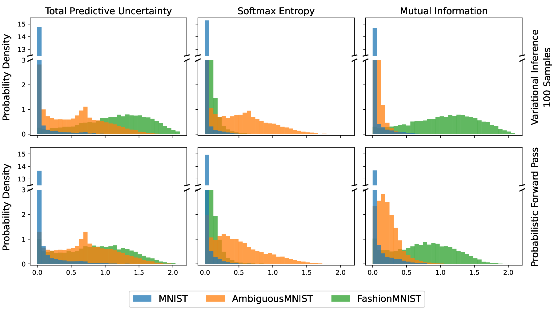
This logit sampling approach is computationally efficient, as it avoids sampling within the network and eliminates the need for multiple forward passes. It serves as a post-processing step, enabling standard uncertainty metrics typically used for sampling-based BNNs. In resource-constrained applications, directly leveraging PFP-predicted variances (𝜎 2 PFP ) for decision-making is an efficient alternative. MNIST AmbiguousMNIST FashionMNIST Fig. 3. Comparison of SVI and PFP uncertainty predictions. For MNIST, both uncertainties are expected to be low; Ambiguous-MNIST exhibits higher aleatoric uncertainty (Softmax Entropy), and Fashion-MNIST, as OOD data, shows higher epistemic uncertainty (Mutual Information). Both methods effectively assign the majority of images to their respective domains. Figure 3 shows that both methods yield higher total predictive uncertainty for Ambiguous-MNIST and Fashion-MNIST compared to the lower uncertainties observed for standard MNIST. Similarly, both exhibit elevated Softmax Entropy for Ambiguous-MNIST, indicating increased aleatoric uncertainty, and higher Mutual Information for the out-of-distribution Fashion-MNIST dataset, reflecting greater epistemic uncertainty. Overall, both approaches provide uncertainty estimates consistent with expectations and desired behavior.

A detailed analysis of Softmax Entropy and Mutual Information across all images, shown in Figure 4, indicates that SVI outperforms PFP in disentangling aleatoric and epistemic uncertainty, as theoretically expected. However, from a practical standpoint, PFP still provides sufficient separation in most cases. Only in certain edge cases do both uncertainties exhibit high values, resulting in less distinct separation.

The Area Under the Receiver Operating Characteristic Curve (AUROC) quantifies a model’s ability to distinguish between in-domain and out-of-domain samples. It is defined as the area under the ROC curve, which plots the true positive rate (TPR) against the false positive rate (FPR) across various thresholds, i.e., AUROC = ∫ 1 0 TPR(FPR -1 (𝑥)) 𝑑𝑥. Thereby a AUROC of 1.0 indicates perfect discrimination, while a score of 0.5 corresponds to random guessing. For a detailed discussion on AUROC computation, refer to [17]. Table 1 presents a comparative analysis of SVI and PFP using AUROC as a metric to evaluate their effectiveness in OOD detection. The results indicate that both methods exhibit comparable performance in terms of predictive accuracy and OOD detection capability.

Furthermore, the influence of the neural architecture is evident, as both methods demonstrate improved predictive performance and OOD detection when utilizing a more expressive convolutional neural network. In summary, PFP achieves prediction quality closely aligned with SVI in both accuracy and OOD detection.

TVM provides multiple internal languages and intermediate representations, including TensorIR [18], TensorExpression (TE), TVMScript, and Relax [33], which are essential for implementing custom operators. While TE defines computational rules in a very succinct way, TensorIR defines the interaction of computations more fine-grained as modular blocks, enabling flexible scheduling and optimizations. 5 Relax [33], the successor to Relay [45], serves as a high-level intermediate representation, supporting dynamic shapes, control flow, and seamless integration with TensorIR. 6 TVMScript, a Python-based frontend, allows the direct definition and modification of TensorIR and Relax.

To implement a custom operator, developers define its computation in TE and create IRModules via the BlockBuilder-API. BlockBuilder creates primitive functions from TE expressions that are connected via Relax and can be optimized using TensorIR scheduling. 7 This workflow facilitates efficient execution of specialized operators across diverse hardware platforms while minimizing implementation complexity.

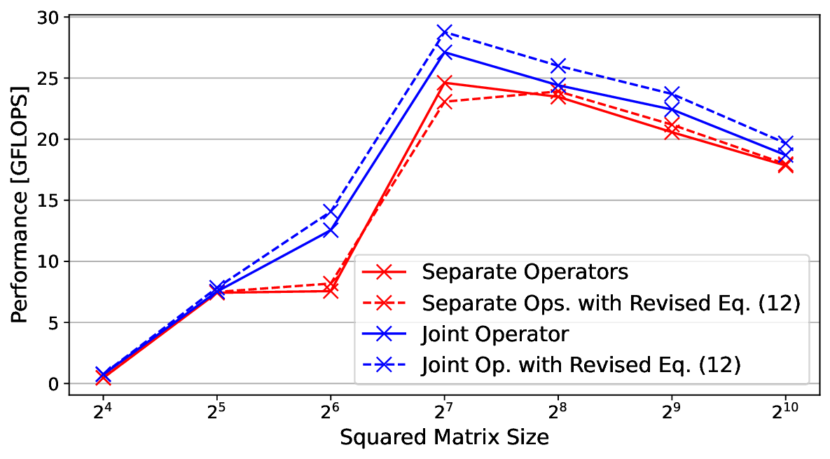
Operating on Tuples. Operators with multiple input tensors are common in neural networks, whereas those producing multiple output tensors are relatively rare. Typically, operators perform a single core computation uniformly across all data. However, PFP introduces a unique requirement, as it maintains separate compute paths and outputs for mean and variance. TVM follows the one operator = one compute rule principle, ensuring that each operator executes a single, sequential stream of instructions without divergence. Consequently, logical PFP operations may be split into separate Separate Operators Separate Ops. with Revised Eq. ( 12) Joint Operator Joint Op. with Revised Eq. ( 12)

Fig. 5. Performance comparison of operator implementations, evaluating the reformulation from Equation 5to 12 and the use of separate vs. joint operators for mean and variance paths on a ARM Cortex-A72.

TVM operators, e.g., one for means and another for variances. However, this approach increases the complexity of interconnecting sub-operators, adds overhead, and complicates the implementation of new network architectures.

Moreover, from a resource efficiency perspective, this separation is undesirable, as mean and variance calculations share common sub-terms. Achieving this integration requires extensions to TVM’s basic operations such as summation over tuples, however, it enables data reuse and eliminates redundant computations. Figure 5 demonstrates that network architectures employing joint operators, as opposed to separate computational paths for mean and variance, consistently benefit from enhanced data reuse. This structural advantage translates into superior performance across all evaluated cases, indicating the efficacy of the joint formulation in leveraging shared intermediate representations.

Variance and Second Raw Moment. The original formulation of PFP operators is based on mean and variance, with inputs and outputs defined accordingly. However, reformulating Equation 5 to operate on second raw moments for activations and weights enhances data reuse and reduces computational overhead. Using second raw moments, the variance in the PFP dense layer can be computed as:

thereby reusing the means for the current layer 𝜇 𝑎 𝑙 𝑖 , the pre-computed second raw moments of the weights E[(𝑤 𝑙 𝑖 𝑗 ) 2 ] and avoiding conversions from previous activation function outputs E[(𝑥 𝑙 -1 𝑗 ) 2 ], which compute second raw moments by design. The locality of this tuple-based second raw moment operator improves cache efficiency and overall performance. When consecutive layers differ in their representation of second raw moments and variances, conversion is straightforward using E(𝑥 2 ) = 𝜇 2 + 𝜎 2 . However, converting second raw moments to variances and then back in subsequent layers introduces unnecessary computational overhead. To mitigate this, the operator implementation includes a conversion function as a configurable argument. Ensuring consistency between the inputs and outputs of connected layers remains the responsibility of the model designer. Moreover, the weights need to be expressed accordingly, either as means and variances 𝜎 2 𝑤 (see (7)) or as means and second raw moments E[𝑤 2 ] (see ( 5)). To minimize redundant computations and facilitate the reuse of intermediate statistical quantities, compute layers-such as dense and convolutional layers-by default expect second raw moments as inputs and produce variances as outputs. Conversely, activation functions expect variances as inputs and produce second raw moments. For architectures 77.5% composed solely of compute layers and activation functions, this default behavior remains consistent. However, when additional layers are introduced, such as Max Pooling layers that both accept and produce variances (e.g., in LeNet-5), the activation function’s output and the compute layer’s input must be converted to variances.

A special case arises in the first layer of the network, where activation uncertainty-and thus variance-is unavailable.

In this scenario, Equations 4 and 12 simplify to:

These equations depend on weight variances, requiring the first layer’s weight variances to be stored in variance format.

For all subsequent compute layers, weight variance information can be stored directly as second raw moments to reduce computational overhead. Additionally, compute layers support three bias configurations: no bias, deterministic bias, and probabilistic bias with variances.

This section analyzed the integration of custom operators into TVM, emphasizing design considerations specific to PFP operators. The evaluation of different implementation strategies demonstrated that the joint operator approach, combined with the second raw moment formulation, provides the highest efficiency in practice.

The PFP implementation presented in Section 5 provides a functional BNN framework capable of uncertainty prediction, as described in Section 4, and is already significantly faster than sampling-based BNNs. However, implementationand hardware-specific safe optimizations can further enhance performance. First, profiling techniques identify the most computationally expensive operators, followed by the application of common optimization strategies to develop a hand-tuned scheduling approach for the MLP. Additionally, we leverage automatic tuning frameworks developed by the TVM community [13,51,55,59]. Finally, we compare PFP implementations across various ARM processor architectures and against SVI-based BNNs. 2 All optimizations in use except tiling.

Efficient optimization requires focusing on the most computationally expensive operators, necessitating a detailed analysis of execution costs per operator. TVM provides three execution modes for compiled binaries: normal execution, benchmarking with advanced averaging for precise measurements, and profiling, which reports per-operator latencies.

These detailed latency reports enable the evaluation of optimization effects on specific operators, as shown in Table 4, and help visualize time distribution per operator, as illustrated in Figure 6.

Figure 6 illustrates the proportion of execution time spent per operator type. For the MLP, dense layers dominate computational costs, whereas in LeNet-5, latency is more evenly distributed across different layer types. This indicates that operators considered simple in a deterministic setting, such as activation functions or pooling layers, can become computationally complex when operating on distributions. This observation is further supported by detailed per-layer latency benchmarks and profiling results obtained with TVM on an ARM Cortex-A72, as shown in Table 4.

The MLP is primarily constrained by the latency of dense layers, making the PFP dense operator the most promising target for optimization. We apply the following techniques, commonly used to accelerate matrix-matrix multiplication, to enhance the efficiency of probabilistic dense operators:

• Tiling: Partitioning matrices into smaller tiles to optimize memory access patterns. Tile sizes must be tuned.

• Loop Reordering: Adjusting loop order to improve vectorization, parallelization, and memory access efficiency.

• Loop Unrolling: Unrolling smaller loops to enhance vectorization and reduce loop overhead.

• Vectorization: Utilizing SIMD instructions efficiently, requiring careful selection of the appropriate dimension.

• Parallelization: Distributing computations across multiple cores while minimizing synchronization and communication overhead.

Table 2 compares the impact of different optimization techniques, evaluating cases where only one optimization is active and where all optimizations except tiling are applied. This allows for an isolated analysis of each technique’s Tiling requires a separate evaluation. When applied independently with hand-tuned tile sizes, it proves highly effective. However, it is the only optimization that does not support stochastic tuning. Since the other optimizations benefit from stochastic tuning, enabling tiling disables this option. As a result, applying all optimizations, including tiling but without stochastic tuning, performs worse than basic tiling alone. The best performance is achieved by combining all other optimizations with stochastic tuning while excluding tiling. Thus, the effectiveness of optimizations is assessed without explicit tiling.

Loop unrolling and parallelization emerge as the most critical optimizations for the PFP dense operator. Combining these techniques results in a substantial speedup of 5× compared to the untuned network.

Max Pool Operator. For LeNet-5, the Max Pooling operator by Roth [46] is formulated as a generic reduction, which is suboptimal in performance. We implement a specialized, vectorized Max Pool operator with fixed kernel size for improved efficiency. As evidenced in Table 3, the application of automatically generated schedules fails to enhance performance and, in fact, results in a substantial deterioration in runtime efficiency. Consequently, this hand-optimized operator is excluded from further automatic tuning.

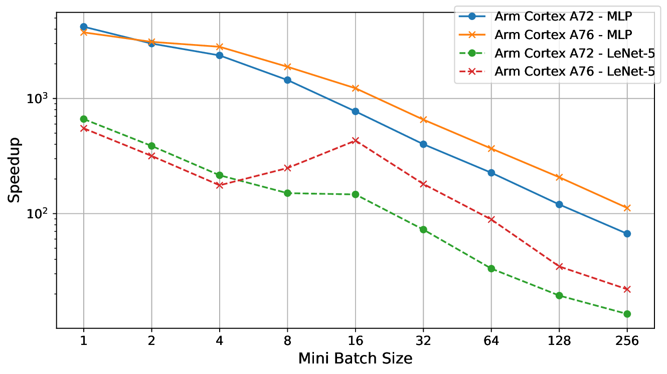
While implementing custom schedules for operators remains common, significant advancements in automatic tuning frameworks have been made by the TVM community [13,51,55,59]. The Meta Scheduler [51] automates schedule generation, eliminating the need for manual implementations. Conceptually, the Meta Scheduler is a domain-specific probabilistic programming abstraction that explores a large optimization search space. Auto-tuning then navigates this space, benchmarking different implementation variants on the target hardware. While this process is slower than expert-crafted schedules, it typically achieves comparable performance and does not require manual effort from domain experts. Applying all optimizations from Table 2, we achieve nearly identical latencies: 0.743 𝑚𝑠 with handwritten schedules and 0.742 𝑚𝑠 with the Meta Scheduler. Thus, the Meta Scheduler proves highly effective, even for specialized PFP operators, and is used for further experiments. 7. Speedup and latency in relation to mini-batch size. The SVI-BNN, evaluated using 30 samples, exhibits high latency and poor scalability for small mini-batch sizes, resulting in significantly higher per-image latency. In contrast, the PFP implementation maintains consistent performance across all mini-batch sizes due to targeted tuning. The observed speedup highlights the advantages of PFP, particularly for small mini-batch sizes, which are critical for low-latency processing in embedded systems.

In resource-constrained embedded systems, real-time and low-latency requirements often necessitate the use of small mini-batch sizes. Figure 7 shows that SVI-based BNNs scale poorly with decreasing mini-batch sizes, incurring substantial computational overhead and high latency per image. To reflect realistic constraints where minimal sample counts are preferred, the SVI-BNN-implemented using Pyro-is evaluated with only 30 samples, which is at the lower bound of the range (see Figure 1b). In contrast, the PFP implementation is optimized per mini-batch size, maintaining relatively stable latency. Only minor latency increases occur when mini-batch sizes misalign with cache or SIMD instruction sizes.

Overall, the performance gap is substantial, reaching multiple orders of magnitude, as illustrated by the speedups in Figure 7b. For a mini-batch size of 256, speedups range from 13× to 112×, while for mini-batch size 1-common in embedded systems-they increase dramatically, reaching 550× to 4200×. On average, PFP is 4.4× slower for the MLP and 11.3× slower for LeNet-5 compared to their deterministic counterparts.

This slowdown is expected due to the increased computational complexity and the doubling of both parameters and activations. However, compared to a state-of-the-art SVI-based BNN with only 30 samples, PFP achieves substantial average speedups of 574× for the MLP and 101× for LeNet-5.

These results highlight the efficiency gains of an approximate SVI approach combined with code generation, demonstrating the feasibility of deploying such models on resource-constrained embedded systems.

Bayesian neural networks empower neural networks with probabilistic reasoning, enabling them to issue warnings when confidence in a prediction is low. Distinguishing between aleatoric and epistemic uncertainty allows identification of inherent stochasticity versus uncertainty due to insufficient training data. In safety-critical applications, such as transportation systems, embedding BNNs in devices enables them to trigger warnings under high uncertainty, allowing human operators to intervene when needed. However, despite these advantages, BNNs are rarely deployed in resource-constrained embedded systems due to their substantial computational and memory overhead compared to non-probabilistic models.

This work advances the deployment of probabilistic machine learning models on embedded systems. We demonstrate how a Stochastic Variational Inference-based BNN can be efficiently executed on embedded ARM CPUs by leveraging the Probabilistic Forward Pass approximation. To achieve this, we extend TVM, a deep learning compiler, to support essential probabilistic operators and optimize them for target hardware architectures.

The Probabilistic Forward Pass mitigates the primary computational bottleneck of BNNs-the need for multiple forward passes per prediction-by assuming Gaussian-distributed weights and activations, enabling a single analytical forward pass. This approach extends the core assumption of SVI-based BNNs, which model weights as parametric distributions, to the activation domain. While this limits the network’s ability to capture complex, non-Gaussian activation distributions, it significantly reduces computational costs when Gaussian approximations are sufficient.

A key advantage of PFP is its compatibility with SVI-trained BNNs, enabling seamless conversion. Our comparative analysis on MNIST, Ambiguous-MNIST, and Fashion-MNIST shows that both approaches achieve comparable predictive performance. While the SVI baseline slightly outperforms PFP in distinguishing aleatoric from epistemic uncertainty, the latter remains equally effective in out-of-domain image detection.

Efficient hardware implementation is essential for deploying probabilistic models on embedded systems. Since they rely on specialized operators for Gaussian distributions-unsupported by standard vendor libraries for machine learning acceleration-we utilize the deep learning compiler TVM. It’s flexibility in implementing and optimizing custom operators across hardware architectures makes it an ideal choice.

Our evaluation of multiple implementation variants shows that joint operators, which compute mean and variance in a single operation, yield greater efficiency. Further optimizations, such as eliminating unnecessary variance conversions and simplifying the first network operators for deterministic inputs, further reduce computational costs.

Following manual optimizations, additional performance gains were achieved through profiling-based operator tuning. We applied targeted optimizations to probabilistic dense operators, developed a more efficient Max Pool operator, and leveraged TVM’s Meta Scheduler for auto-tuning. As a result, our optimized Probabilistic Forward Pass implementation achieved a two-order-of-magnitude speedup over the SVI-based BNN baseline on ARM processors.

For small mini-batch sizes, which are critical for low-latency embedded applications, speedups of up to 4200× were achieved.

To our knowledge, this work presents the first end-to-end demonstration of training, optimization, and deployment of Bayesian neural networks on resource-constrained embedded systems. Our findings illustrate that integrating Bayesian approximations with deep learning compilers enables the deployment of otherwise computationally prohibitive probabilistic models. We hope this work marks the beginning of further research bridging the gap between resourceintensive probabilistic models and constrained embedded hardware-bringing uncertainty-aware neural networks into everyday devices and enabling them to acknowledge uncertainty by saying, “I don’t know. "

In San Francisco

a driverless car just got stuck in wet concrete, since it was unaware of the situation that wet concrete exists. https://www.nytimes . com/2023/08/17/us/driverless-car-accident-sf.html

The code is available at: https://github.com/UniHD-CEG/PFP-Operator-Library

https://mc-stan.org/

https://github.com/tensorflow/probability

https://tvm.apache.org/docs/deep_dive/tensor_ir/tutorials/tir_creation.html

https://tvm.apache.org/docs/deep_dive/relax/learning.html

https://mlc.ai/docs/get_started/tutorials/quick_start.html