A Fast and Flat Federated Learning Method via Weighted Momentum and Sharpness-Aware Minimization

FL in edge computing has several unique attributes. To reduce communication costs, the number of local iterations must increase. Concurrently, partial participation is often used due to the unstable connectivity of IoT devices. These two factors exacerbate the harmful effects of data heterogeneity [8][9][10] in real-world applications, intensifying client drift [11], where local updates deviate significantly from the global objective, degrading model performance and generalization.

Local multi-round training increases the drift caused by data heterogeneity, while partial participation further magnifies its effects. Based on where the drift originates, current methods for mitigating client drift can be categorized into the following levels: Methods at the data level attempt to balance data distribution through techniques such as data augmentation [12,13] or resampling [8,14], but these methods may incur high computational costs and risk overfitting. Gradient-level approaches, including proximal methods [9], gradient correction [11], and regularization terms [15], aim to adjust local gradients, but gradient distortion may hinder convergence. Techniques for model aggregation [16][17][18] alter the server’s aggregation strategy, requiring the collection of additional information that may conflict with the privacy principles central to FL. At the same time, cryptographic PPFL (e.g., HE) offers an alternative at the cost of efficiency [19,20].

Moreover, on the one hand, these methods focus solely on addressing client drift, with little consideration for convergence speed, while fewer training rounds could enhance real-world applicability. On the other hand, when heterogeneity is high, the loss surface resulting from aggregating models trained with Empirical Risk Minimization (ERM) becomes sharp, limiting the models’ generalization in practical applications. Moreover, in non-IID FL, we observe two structural failure modes when simply porting SAM and/or momentum: (i) localglobal curvature misalignmentlocal SAM directions need not reflect the global loss geometry; (ii) momentum-echo oscillationlate-stage instability caused by accumulated momentum. These motivate a design that can both align local updates to the global geometry and adaptively damp momentum as training progresses.

To solve this problem, we aim to design a fast and flat FL algorithm. Two mainstream lines address the twin goals in FL: momentum [21][22][23][24][25] for speed and SAM [26][27][28] for flatness. However, under non-IID data, each line has structural drawbacks: momentum can amplify late-stage instability/overfitting [29], while SAM requires an extra backward pass and, more importantly, its local perturbation directions need not reflect the global loss geometry (the localglobal curvature misalignment diagnosed above). Momentum-only designs tailored to long-tailed heterogeneity (e.g., FedWCM [24,25]) improve robustness but do not enforce global flatness.

A straightforward combination existsMoFedSAM inserts SAM into FedCM [26,22]yet naively plugging SAM into a momentum pipeline leaves the two failure modes unresolved in non-IID settings (misalignment persists, late-stage momentum oscillation is not damped). This motivates a design that both aligns local updates to the global geometry and adaptively damps momentum as training progresses, we instantiate this next as FedWMSAM.

To address the aforementioned issues and achieve fast and flat training in FL, we propose Fed-WMSAM (Federated Learning with Weighted MomentumSAM), which integrates momentum with SAM in a principled way.

• Firstly, we introduce personalized momentum and use the server-aggregated momentum as a global geometric carrier to build a momentum-guided global perturbation, aligning local SAM directions with the global descent geometry; the perturbation is implemented with a single backpropagation (no extra backward pass).

• Secondly, we dynamically adjust the perturbation along this global direction during local steps (e.g., xr b = x r + b ∆ r ), enabling each client to explore globally flatter regions without increasing per-round cost.

• Thirdly, we couple momentum and SAM via a cosine-similarity adaptive weight α r , which yields an early-momentum / late-SAM two-phase schedulespeeding up early progress while damping late-stage momentum oscillations under non-IID data.

Our main contributions are summarized as follows:

• Mechanism. We identify and formalize two failure modes in non-IID FLlocalglobal curvature misalignment and momentum-echo oscillationand correct them via a momentum-guided global perturbation and a cosine-adaptive coupling. 2 Related Work

Federated learning (FL) often encounters the challenge of client drift. Existing solutions can be divided into three levels: data, gradient, and aggregation. At the data level, resampling strategies [14] adjust local sampling probabilities to balance class distributions, generative models like GANs [12] and VAEs [13] synthesize balanced datasets, and data-sharing approaches [8] distribute small portions of global data to clients. At the gradient level, methods such as SCAFFOLD [11] reduce variance using control variates, FedDyn [15] applies dynamic regularization, FedProx [9] stabilizes updates with proximal terms, and FedCM [22] aligns updates via momentum correction. At the aggregation level, Hierarchical FL [17] applies multi-level aggregation for large-scale networks, Clustered FL [16] groups clients with similar data distributions for localized optimization, and works like Client Selection [30] and Client Weighting [18] adjust the influence of clients based on their contribution to the global model. However, these works focus solely on addressing heterogeneity data, neglecting speed and model generalization.

Utilizing historical gradient information via momentum has proven effective for accelerating convergence and handling data heterogeneity in FL. The fundamental idea is to constrain current updates by past directions, smoothing out oscillations. MIME [21] and FedCM [22] compute a global momentum on the server and distribute it for stricter consistency, while AdaBest [31], FedADC [32], and ComFed [33] adaptively calculate local momentum on clients and synchronize each round. Methods like MFL [34] and FedMIM [23] entirely apply momentum on-device to reduce communication. In parallel, momentum-based designs specifically tailored for long-tailed non-IID heterogeneity, such as FedWCM [24,25], provide an efficient complementary approach. Although momentum mechanisms significantly improve early-stage convergence in non-IID scenarios, they can sometimes hinder late-stage fine-tuning, causing notable performance fluctuations.

Model generalization is closely tied to finding flatter regions of the loss surface, motivating Sharpness-Aware Minimization (SAM) [35]. SAM actively seeks flatter optima and reduces overfitting risks by perturbing the model around local minima. In the federated setting, works like Fed-SAM [26], MoFedSAM [26], and FedGAMMA [27] plug SAM optimizers into FedAvg, FedCM, or SCAFFOLD but do not explicitly refine the global flatness search. FedSMOO [28] integrates FedDyn regularization to minimize local-global bias, whereas FedLESAM [36] estimates global perturbations based on local-server discrepancies. More recently, FedGloss [37] extends FedSMOO by leveraging the global pseudo-gradient from the previous round to reduce communication costs, while FedSFA [38] selectively applies SAM perturbations using historical information to lower computational cost. While these approaches enhance generalization, exploring flat minima inevitably slows convergence, and SAM’s two backward passes increase computational overhead, further complicating its practical deployment in heterogeneous FL.

Federated Learning (FL) [1] enables multiple clients to train a global model collaboratively while preserving data privacy. The objective is

, where v r k is the momentum at client k in round r, α is the momentum factor, g r k is the local gradient, and ∆ r is the global momentum. Methods like MIME and FedCM employ this scheme to coordinate and stabilize local optimization under non-IID conditions.

Sharpness-Aware Minimization (SAM) [35] improves generalization by identifying flatter regions of the loss function. Its objective is:

Implementation typically involves two steps: (1) compute δ = ρ ∇F (w) ∥∇F (w)∥ and (2) update model parameters w based on the perturbed gradient L(w + δ). This forces the model to converge to flatter minima by explicitly considering the worst-case local perturbation.

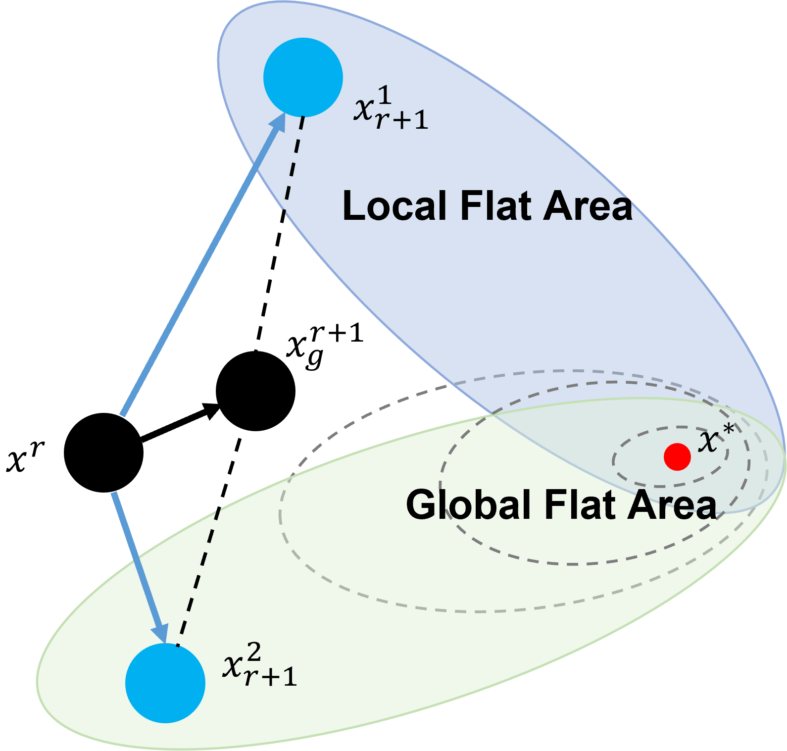
The core challenge of applying SAM in federated learning lies in a fundamental mismatch: SAM computes perturbations based on local data, but aims to find flat minima in the global landscape (Figure 1). Due to data heterogeneity, these local perturbations often fail to accurately reflect the global geometry, thereby limiting the effectiveness of SAM in federated settings.

To resolve this contradiction, existing methods attempt to either reduce the discrepancy between local and global models or improve the estimation of global-aware perturbations using local information. However, as analyzed in Appendix A, these approaches still fall short in fully bridging the local-global gap, motivating the need for a more unified and efficient solution. This motivates us to propose a new approach that more effectively integrates SAM with federated optimization. This section presents our FedWMSAM algorithm, which fuses personalized momentum and SAM for federated optimization. Section 4.1 highlights our methodology and illustrates the three key components (personalized momentum, global perturbation estimation, and dynamic weighting). Section 4.2 then details the implementation, including pseudocode, the computation of personalized momentum ∆ k r and dynamic weight α r .

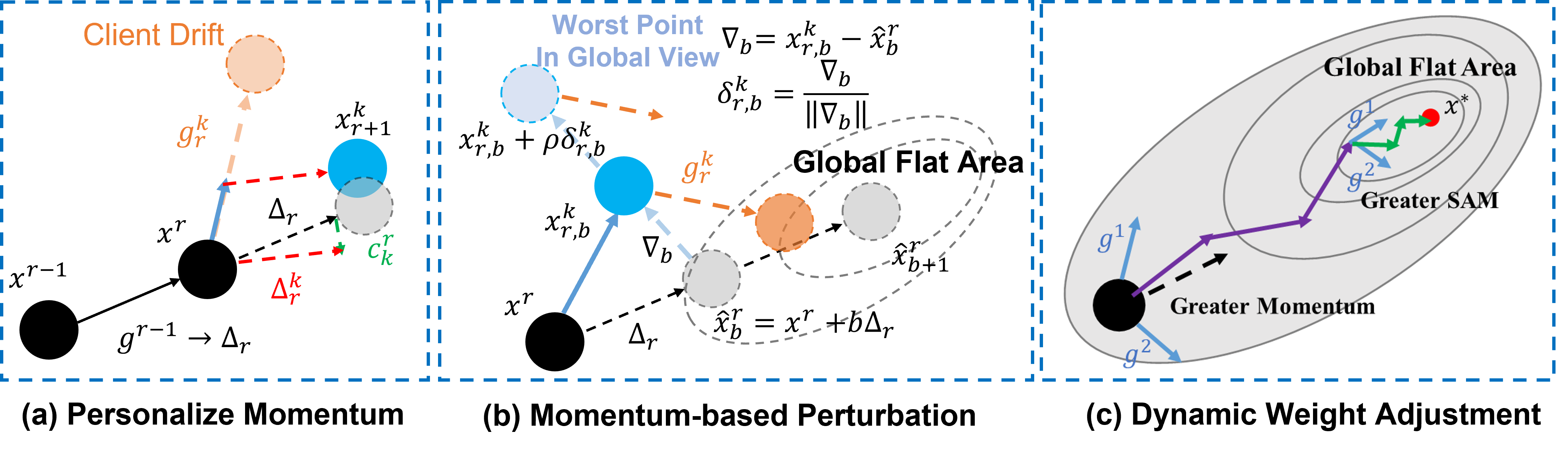
(a) Personalized momentum for local-global discrepancy. We use the diagram in Figure 2 (a) to illustrate the concept of personalized momentum. In FedCM [22], momentum utilizes the previous gradients to guide the next round of local training, which can effectively accelerate model convergence, as the black dashed line shows. However, it is worth noting that although each client has different data distributions, they share the same momentum. Although momentum mitigates part of the bias introduced by local gradients, the drift caused by data heterogeneity recurs in every communication round and cannot be fully corrected by momentum alone. Based on this, we introduce a correction term c from SCAFFOLD to estimate the bias caused by local data using historical experience. Unlike the original SCAFFOLD [11], which requires uploading local correction terms in each round for global averaging and redistribution, our approach only requires the server to compute the correction term based on the differences in gradients uploaded by clients. This correction term c r k in the green dashed line is then aggregated with the momentum ∆ r to form personalized momentum ∆ k r , as shown in the red dashed line, effectively saving communication bandwidth. At each step, we calculate the difference between the current model and the inferred global model, using ∇ b in light blue dashed line as the perturbation direction, based on the analysis that the direction of deviation from the global model indicates regions of higher loss. By doing this, we eliminate the need for an additional backpropagation step to compute the perturbation while improving the estimation of the global perturbation.

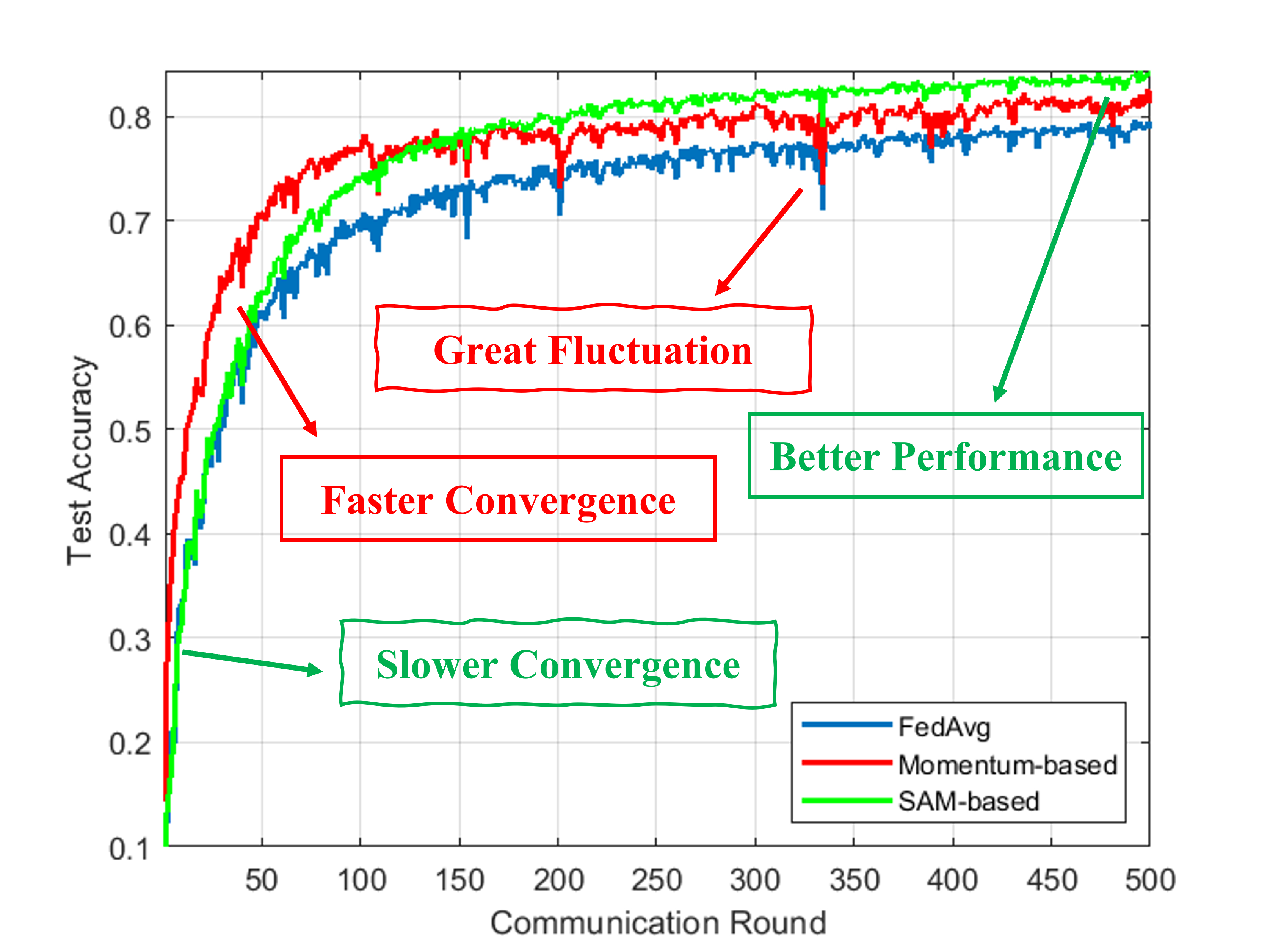
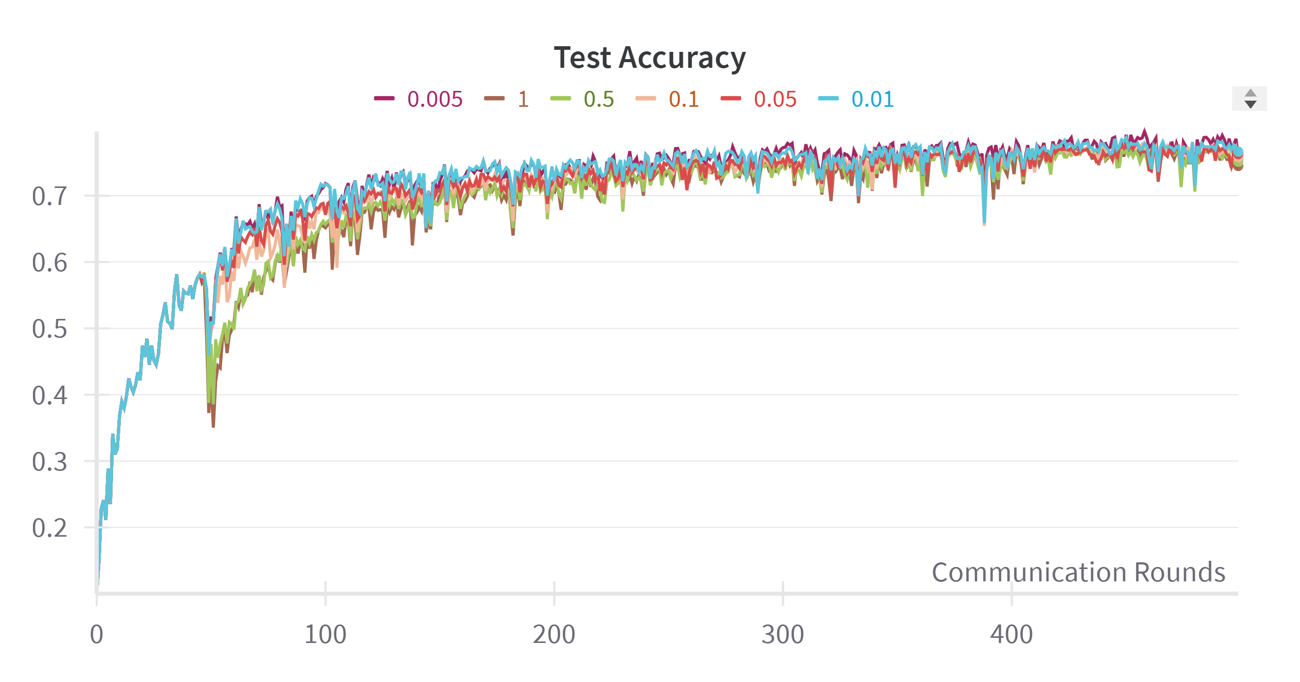
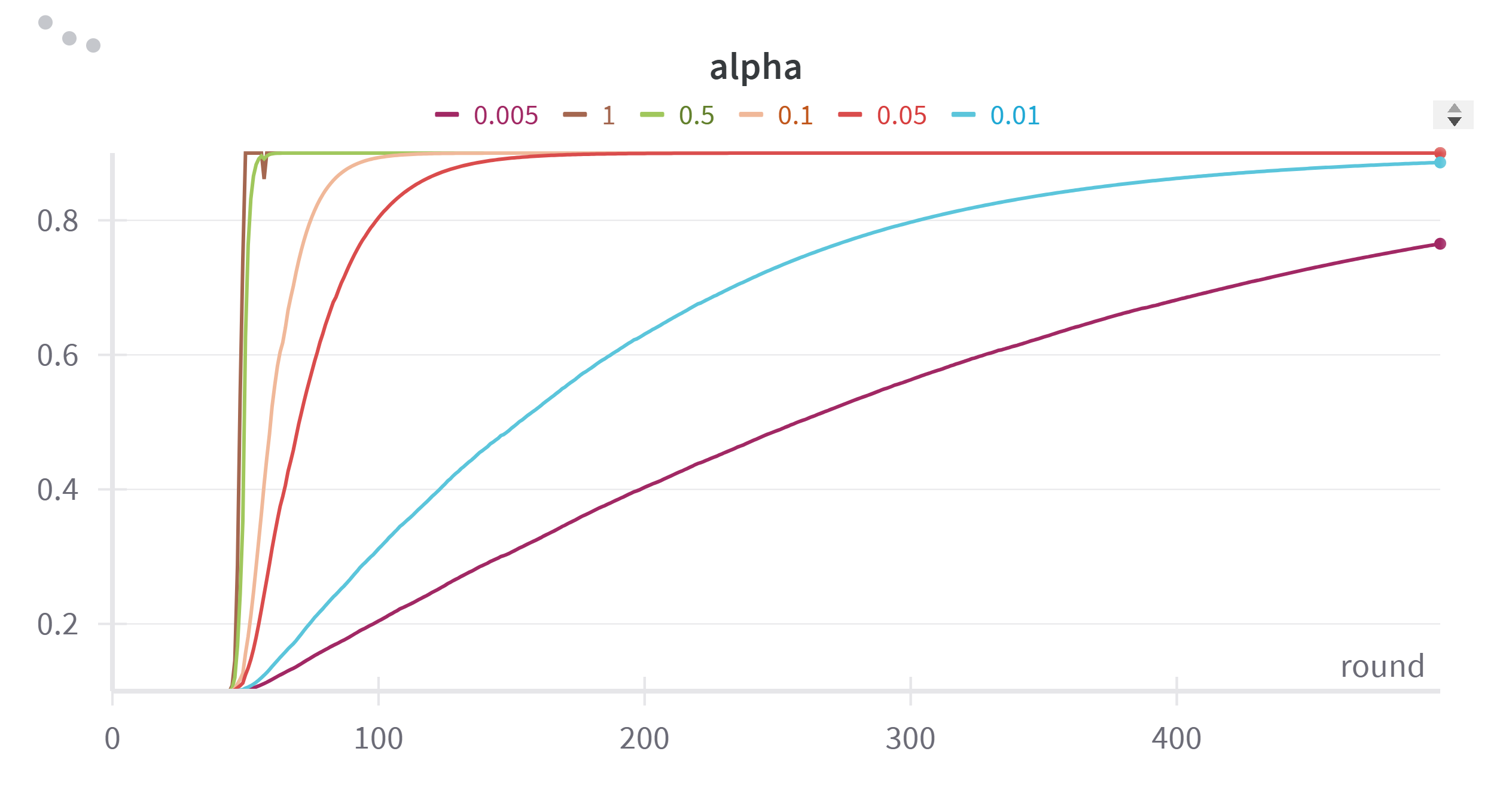
(c) Dynamic Weighting via GradientMomentum Similarity. Although momentum accelerates early convergence and SAM improves final accuracy, their roles vary throughout the training process. An overly significant momentum can hinder late-stage fine-tuning, while pure SAM is relatively slow, as shown in Figure 3. Inspired by experiments conducted by Andriushchenko et al. [39], which show that switching from ERM to SAM at different epochs can lead to varying test errors, we realized that it is crucial to determine the optimal time to increase the weight of SAM. We observe that the cosine similarity between clients’ directions and the global signal increases early and stabilizes later (see Appendix B), so we increase α r monotonically with the similarity-yielding early-momentum, late-SAM. This allows us to rely more on momentum during the early stages and gradually weaken its influence to better explore the global flat region in the final stages. Figure 2 (c) shows how momentum is helpful to speed up initially in the purple line, then gradually yields to SAM for robust final convergence in the green line.

In this section, we describe the components and procedures of the FedWMSAM algorithm. First, we provide an overview of the method, followed by detailed explanations of each component. Algorithm 1 summarizes the overall procedure.

At each communication round r, the server selects a subset of clients P r and computes each client’s personalized momentum. The server then broadcasts the global model x r , the personalized momentum ∆ k r , and the momentum factor α r to the selected clients. Each client updates its model using the global momentum and performs local updates with SAM perturbation. The momentum factor is adapted based on cosine similarity, and personalized corrections are refined following the SCAFFOLD-like method to reduce local-global drift. Next, we explain each of these steps in detail.

At each round r, the server computes the personalized momentum for each selected client k by:

where ∆ r is the global momentum, α r is the momentum factor, and c k is the local correction for client k. This step ensures the alignment of the global and local updates. The coefficient αr 1-αr arises because, during the local updates, the momentum term is combined with the gradient as:

We want the correction term c k to affect the gradient g r b,k directly, so the coefficient αr 1-αr is used to scale c k in the global momentum computation. This adjustment ensures that c k has the same effect on the gradient as it would in the local update, enabling a consistent blend of global and local dynamics in the personalized momentum. This transformation decouples the correction term from momentum, reducing the need to transmit separate vectors for momentum and correction and saving bandwidth.

After each round, we update the momentum factor α r+1 based on the cosine similarity between the global momentum and each client’s personalized momentum. For efficiency, we compute the similarity using sim(∆ r , ∆ k r ), which we empirically find to be a good proxy for the gradientmomentum similarity without incurring extra backpropagation (see Appendix B). The updated momentum factor is:

and the final update is:

where λ controls the speed of adaptation. The choice of the bounds for α r+1 , specifically within the range [0.1, 0.9), is motivated by several factors. Based on the analysis in [22], a momentum factor of 0.1 yields the best performance. This setting ensures that the momentum gradually decreases over time, allowing the SAM perturbation to become more prominent in later rounds. Therefore, the upper bound of 0.9 ensures that momentum remains sufficiently large, maintaining its influence on the calculation of SAM, which relies on the momentum term. The lower bound 0.1 prevents the momentum weight 1 -α r from vanishing too early, while the upper bound 0.9 avoids over-reliance on momentum so that SAM can dominate in later rounds. More discussion of this choice of the value can be found in Appendix B.

Finally, the server updates the personalized correction terms c k and c g using a SCAFFOLD-inspired strategy [11]. These updates help reduce local-global drift and refine the correction offsets for each client and are calculated as:

Algorithm 1 FedWMSAM Require: Initial model x 0 , global momentum ∆ 0 , correctors c g , c k , momentum factor α 0 = 0.1, learning rates η l , η g , perturbation magnitude ρ, communication rounds R, local iters B

for each client k ∈ P r in parallel do

Compute ∆ k r using Eq. ( 1)

4:

end for 6:

Compute α r+1 using Eq. ( 3) and ( 4)

Update c g , c k using Eq. ( 5) 10: end for Ensure:

We provide a non-IID convergence guarantee for FedWMSAM, with a rate of

. Our analysis builds upon the SCAFFOLD-M framework [40], and explicitly accounts for the perturbation-induced variance σ 2 ρ = σ 2 + (Lρ) 2 , with two key extensions: an adaptive personalized momentum term and the integration of SAM. Notably, we show that the variance induced by SAM is bounded by the perturbation strength ρ. The complete proof and comparisons with related convergence rates are presented in Appendix A.

We propose FedWMSAM and compare it with existing SOTA federated SAM methods, including FedSAM [26], MoFedSAM [26], FedGAMMA [27], and FedSMOO [28], as well as FedLE-SAM [36] and its two variants, FedLESAM-S and FedLESAM-D. Since our method incorporates momentum and correction terms, we also compare it with classical federated optimization baselines such as FedAvg [1], FedCM [22], and SCAFFOLD [11]. By default, we set p k,c ∼ Dir(β), where p k,c denotes the class distribution of client k over class c, and β = 0.1. The main experiments are conducted with 100 clients, 10% participation per round, a batch size of 50, a local learning rate η l = 0.1, a global learning rate η g = 1, and five local epochs, running for 500 communication rounds. For Fashion-MNIST [41], we use a Multi-Layer Perceptron (MLP) architecture. For CIFAR-10 [42], we use ResNet-18 [43] as the backbone, ResNet-34 [43] for CIFAR-100 [42], and ResNet-50 [43] for OfficeHome. Each domain in OfficeHome is divided into one client with 10% data sample rate and 100% active ratio. The perturbation magnitude ρ is set to 0.01 for FedSAM, FedGAMMA, FedLESAM, and our FedWMSAM, while FedSMOO and MoFedSAM use ρ = 0.1 by default. Additional experimental settings are detailed in the corresponding figures and tables. All experiments were implemented in PyTorch and conducted on a workstation with four NVIDIA GeForce RTX 3090 GPUs.

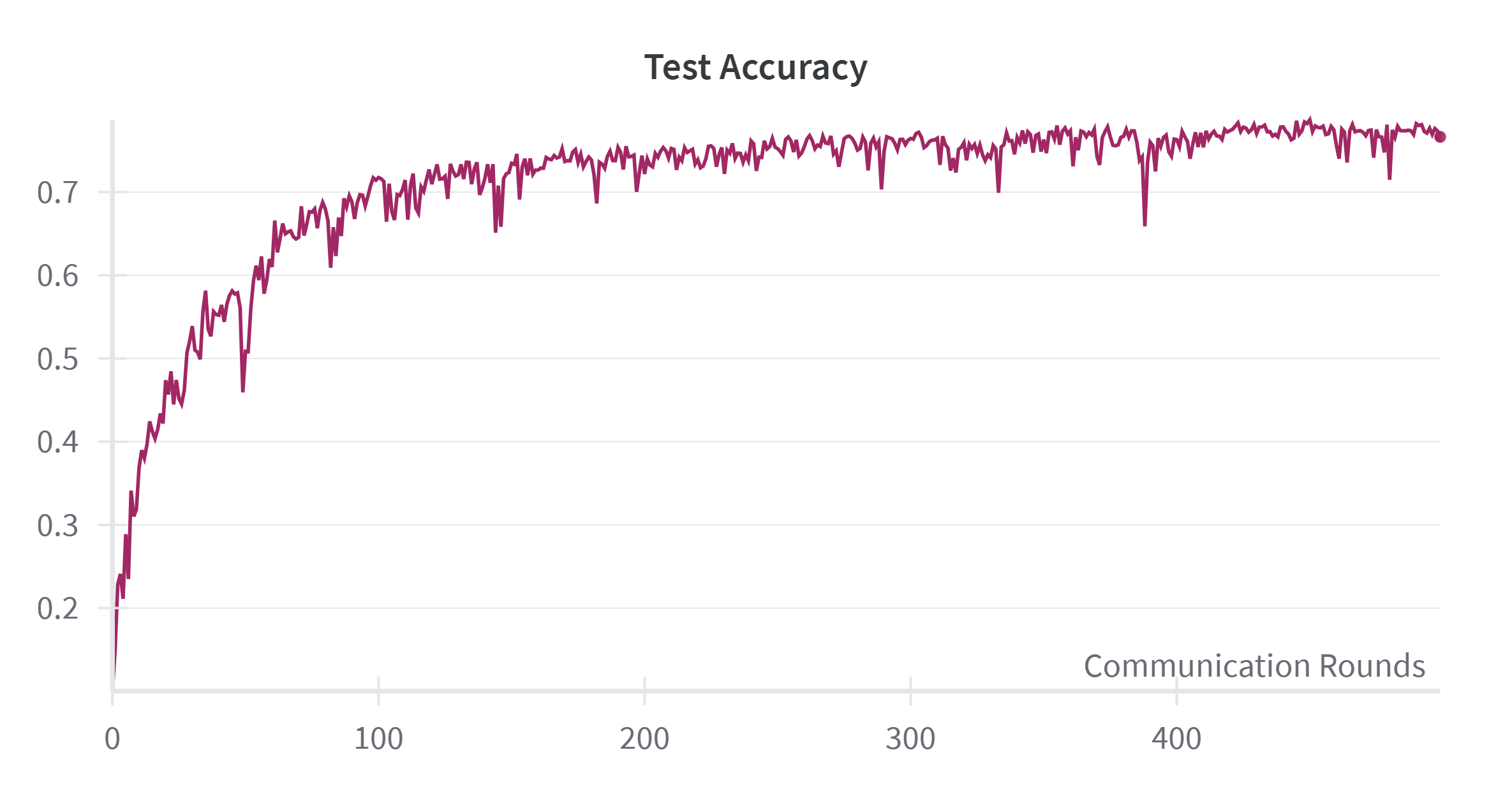
Accuracy Evaluation. Table 1 summarizes results across three datasets and twelve heterogeneity settings. FedWMSAM is best or second-best in most cases, with the advantage most pronounced under stronger non-IID settings (β=0.1 and pathological splits). Specifically, on CIFAR-10/100 at β=0.1 we achieve 76.64%/46.46%, improving over baseline FedAvg by +6.59/+8.31 points. Similarly, under scenarios where γ = 3 for CIFAR-10 and γ = 10 for CIFAR-100, FedWMSAM attains accuracies of 74.46% and 43.83%, surpassing FedAvg by +10.2 and +7.52 points, respectively. Mechanistically, the cosine-similarity adaptive coupling induces an early-momentum, late-SAM two-phase behavior that dampens momentum-echo oscillation, yielding the observed fast-then-flat trajectories.

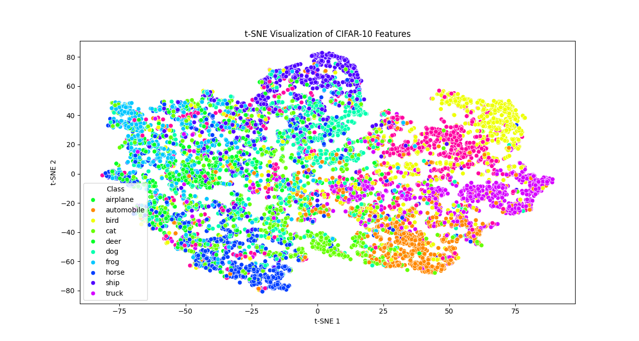
Generalization Illustration. To intuitively illustrate the generalization ability of our method, we present the t-SNE visualization of the global models trained by four FL algorithms on CIFAR-10: FedAvg, FedSAM, MoFedSAM, and our FedWMSAM. As shown in Figure 5

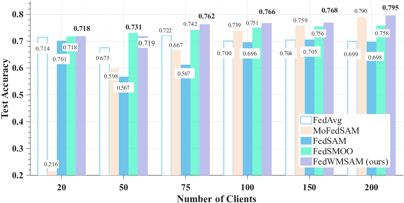
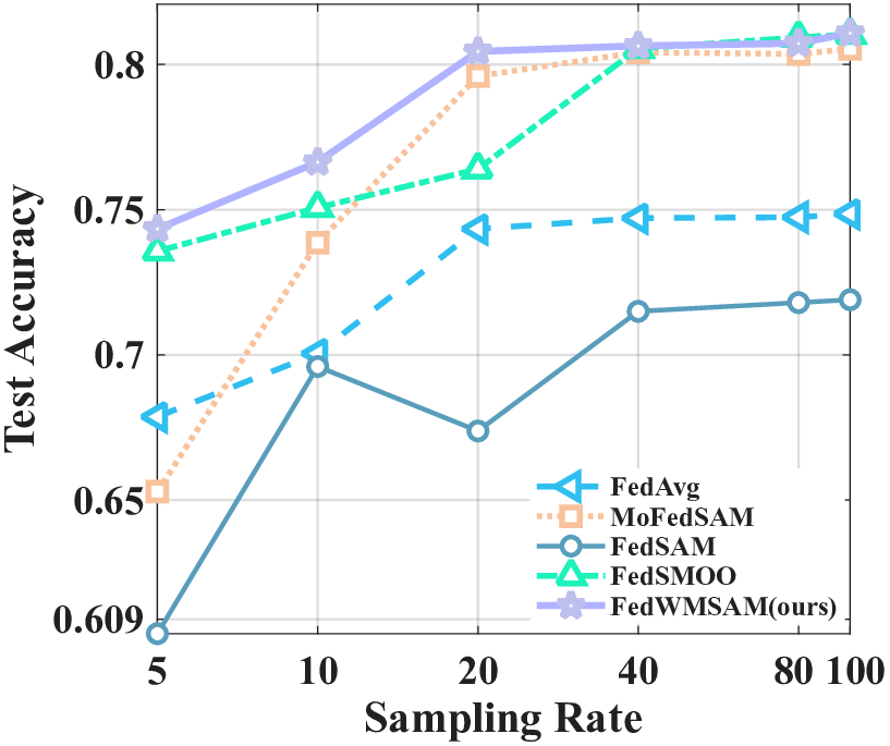
To validate the adaptability of our method to various experimental settings, we study sensitivity along three axes: (i) local epochs, (ii) number of clients, and (iii) client sampling rate, comparing it with FedAvg and SAM-family baselines ( MoFedSAM, FedSAM, and FedSMOO). We conducted ablation studies on our method and the perturbation coefficient ρ to validate its systematic design and parameter choices. We ablate three modules: personalized momentum (Mom.), momentum-guided SAM (SAM, single backprop), and the cosineadaptive weight (Weighted; α r ). The bottom row (×/×/×) corresponds to FedCM (no personalized momentum, no SAM, no adaptive coupling), and the Imp. is computed over FedCM.

Table 5 presents the performance of different component combinations. The personalized momentum primarily reduces local-global bias, which accounts for the significant gains observed with the Mom.-only approach.

The cosine-adaptive rule serves as a data-driven damping mechanism. When both Mom.& SAM exist, it facilitates an early-Mon. and late-SAM schedule. This combination helps suppress momentum echo and enhances the final performance plateau. In contrast, when SAM is not present, the same gate may diminish the momentums acceleration and bring only marginal benefit. Overall, the three modules work together complementarily: Mom. fixes bias, SAM supplies flatness, and Weighted harmonizes the two. We further vary the perturbation magnitude ρ. Table 6 shows that accuracy peaks around ρ=0.01, and FedWMSAM degrades gracefully as ρ increases (0.7664 → 0.7563 → 0.7244 → 0.5905 from 0.01 → 0.05 → 0.1→ 0.5), whereas MoFed-SAM collapses at large ρ (0.7102 → 0.5562 → 0.1000).

Our momentum-guided perturbation aligns the SAM direction with the global geometry. The cosineadaptive weight reduces SAM’s contribution when there is misalignment or noise. This results in a milder effective perturbation during noisy rounds, which corresponds to the bounds dependence on σ 2 ρ = σ 2 + (Lρ) 2 . As ρ increases, the noise term also rises, but the adaptive gate mitigates its effect, preventing the catastrophic failure observed in MoFedSAM.

We provide additional experiments in Appendix B and Appendix C. Appendix B includes studies on the cosine-based computation of α r and the effect of decay coefficient λ. Appendix C presents additional results and visualizations across datasets and partitioning settings, offering more detailed comparisons that support the robustness of FedWMSAM.

In this paper, we addressed why naively combining momentum and SAM under non-IID FL underperforms by identifying and formalizing two failure modes: localglobal curvature misalignment and momentum-echo oscillation. We introduced FedWMSAM, which (i) builds a momentum-guided global perturbation to align local SAM directions with the global descent geometry (single backprop), and (ii) couples momentum and SAM via a cosine-similarity adaptive rule that yields an early-momentum / late-SAM two-phase schedule. On the theory side, we gave a non-IID convergence bound that explicitly models the perturbation-induced variance σ 2 ρ =σ 2 +(Lρ) 2 and its dependence on (S, K, R, N ). Empirically, across three datasets and twelve heterogeneity settings, FedWMSAM is best or on-par in most cases, with the largest gains in strong non-IID, and it reaches target accuracies in fewer rounds while maintaining near-FedAvg per-round cost, realizing the intended fast-and-flat optimization. Throughout the proofs, we use i to represent the sum over i ∈ {1, . . . , N }, while i∈Sr denotes the sum over i ∈ S r . Similarly, we use k to represent the sum over k ∈ {0, . . . , K -1}. For all r ≥ 0, we define the following auxiliary variables to facilitate proofs:

Throughout the appendix, we let

]. We will use the following foundational lemma for all our algorithms. Assumption 1 (Standard Smoothness). Each local objective f i is L-smooth, i.e., ∥∇f i (x) -∇f i (y)∥ ≤ L∥x -y∥, for all x, y ∈ R d and 1 ≤ i ≤ N .

There exists σ ≥ 0 such that for any x ∈ R d and

Lemma 1. Under Assumption 1, if γL ≤ 1 24 , the following holds for all r ≥ 0:

Since x r+1 = x r -γg r+1 , using Young’s inequality, we further have

where the last inequality is due to γL ≤ 1 24 . Taking the global expectation completes the proof.

If they are correlated in the Markov way such that E

, the variables {X i -µ i } form a martingale. Then the following tighter bound holds:

Proof. Letting {i ∈ S} be the indicator for the event i ∈ S r , we prove this lemma by direct calculation as follows:

Lemma 4 (Perturbation-Induced Gradient Variance). Suppose each local objective f i is L-smooth (Assumption 1), and the stochastic gradient ∇F (x; ξ i ) is unbiased with variance at most σ 2 (Assumption 2). Then for any x ∈ R d , any client i, and any perturbation vector δ with ∥δ∥ ≤ ρ, we have

Proof. By definition, the random gradient can be decomposed as

We denote these two terms by A and B, respectively. Then

From Assumption 2 (Stochastic Gradient), we know

and

By Assumption 1 (L-smoothness), we have

Hence,

Since B is deterministic w.r.t. ξ i , we have

Thus in expectation,

Putting it all together gives

as claimed.

Following the sketch of SCAFFOLD-M [40], we proceed to prove the convergence of FedWMSAM. We begin by considering the following lemma: Lemma 5. If γL ≤ 1 2αr , the following holds for r ≥ 1:

where σ 2 ρ denotes σ 2 + (L ρ) 2 . In addition,

Proof. According to the definition of personalized momentum in FedWMSAM, denoting g i r as the personalized momentum of client i in round r, we have

Note that 1 N N i=1 c r i = c r holds for any r ≥ 0. Using Lemma 3, E r can be expressed as:

To simplify, we define:

Thus, E r can be rewritten as:

For r ≥ 1, expand Λ 1 we can get,

Note that {∇F (x r,k i +δ r,k i ; ξ r,k i )} 0≤k<K are sequentially correlated. Applying the AM-GM inequality, Lemma 2 and 4, we have

Let σ 2 ρ denote σ 2 + (L ρ) 2 , which corresponds to the variance of the client’s gradient after the perturbation is added. Using the AM-GM inequality again and Assumption 1, we have

Finally,

where we plug in ∥x r -x r-1 ∥ 2 ≤ 2γ 2 (∥∇f (x r-1 )∥ 2 + ∥g r -∇f (x r-1 )∥ 2 ) and use γL ≤ αr 6 in the last inequality. Similarly for r = 0,

Besides, by the AM-GM inequality and Lemma 1 and 4,

Since

The case is similar for r = 0,

Then, from the definition of U r as the expected squared difference between each local model after K local updates and the averaged model, we have:

where the bound follows by analyzing the variance and bias accumulation over K local steps.

Next, we estimate Ξ r , the average squared norm of the update direction:

Substituting the bound of Ξ r back into the expression for U r , we obtain: 2 , which proves the lemma. Lemma 7. Under the same conditions as Lemma 6, if α r ηKL ≤ 1 24K 1/4 and ηK ≤ 5γ N S , then we have

Proof. Since

Using Youngs inequality repeatedly, we have

Here we apply Lemma 1 to obtain the second inequality. Combining this with Lemma6, we have

Finally,

where we apply the upper bound of η. Therefore, we finish the proof by summing up over r from 0 to R -1 and rearranging the inequality.

Theorem 1. Under Assumption 1 and 2, if we take g 0 = 0,

then FedWMSAM converges as

Proof. By Lemma 5, summing over r from 0 to R -1 and plugging Lemma 6 and 7 in, we have

Here, the coefficients in the last inequality are derived by the following bounds:

which can be guaranteed by

Combining this inequality with Lemma1, we obtain

Finally, noticing that g 0 = 0 implies E -1 ≤ 2L∆ and

Table 7 summarizes the theoretical convergence rates of FedWMSAM and several representative federated optimization algorithms under non-convex settings. These methods differ in their design focusessome emphasize global convergence guarantees, while others incorporate mechanisms for bias correction or perturbation modeling.

Our proposed FedWMSAM achieves the following convergence bound:

where the first term captures the influence of gradient noise introduced by sharpness-aware perturbations, and the second term reflects the effects of client sampling and system heterogeneity.

This result highlights three key aspects of FedWMSAM:

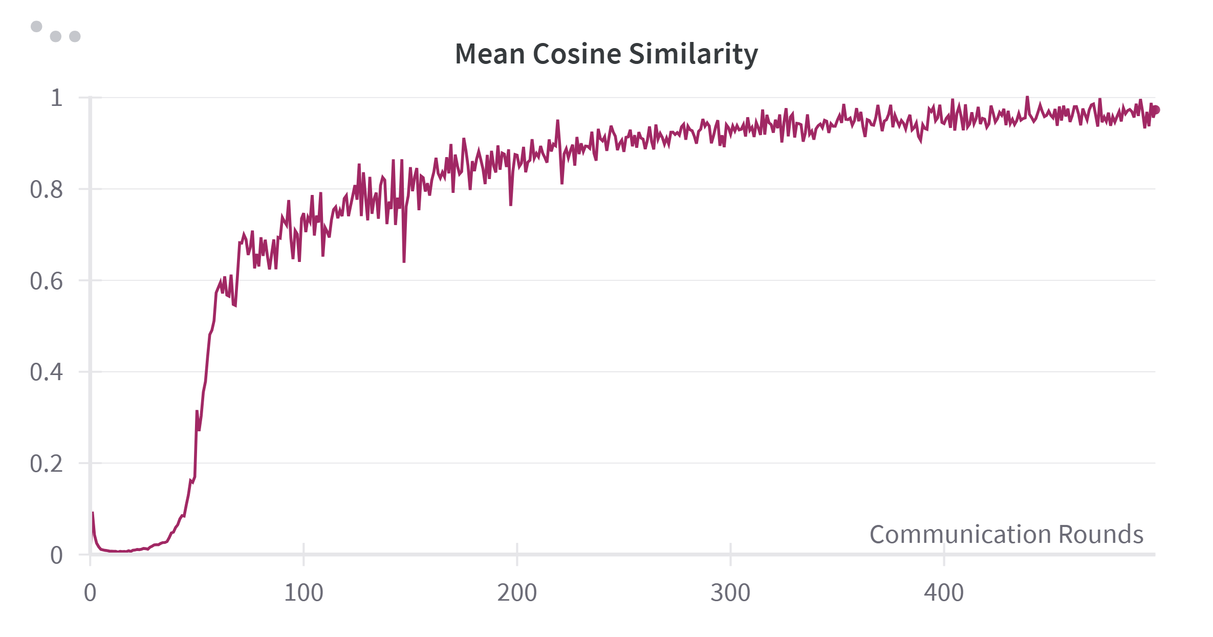
1. It explicitly models the impact of perturbation-induced gradient variance σ 2 ρ , improving robustness in sharp-loss regions; The training process typically enters its later stages when the test accuracy stabilizes. We examined the relationship between the cosine similarity and accuracy by plotting their respective trends. As shown in Figure 7, the cosine similarity increases rapidly around the 50th round and reaches a steady state after around 200 rounds. This aligns with the accuracy curve shown in Figure 8, where accuracy also rises quickly before 50 rounds, decelerates between 50 and 200 rounds, and then stabilizes after 200 rounds.

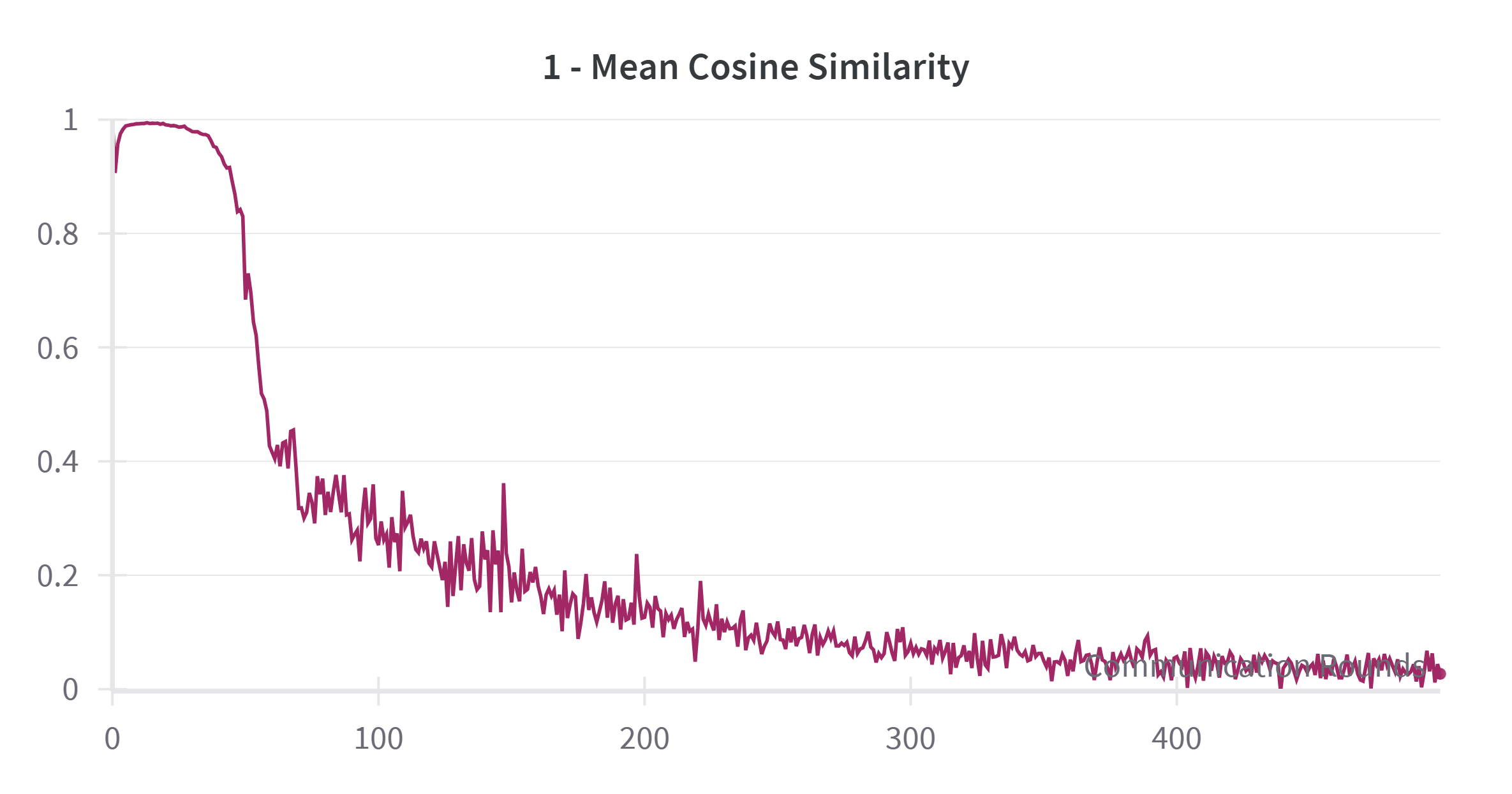
From this analysis, we observe a negative correlation between the Mean Cosine Similarity and the speed of accuracy improvement. Specifically, the slope of the accuracy curve appears to be approximately one minus the cosine similarity. To further explore this relationship, we plotted one minus the cosine similarity value in Figure 9. The plot clearly demonstrates that a higher cosine similarity corresponds to a more rapid increase in test accuracy, while lower similarity values indicate slower accuracy growth.

Based on these findings, we established a clear connection between test accuracy and cosine similarity, which can be used to estimate the training period. As discussed previously, the momentum should have a more substantial influence in the earlier stages of training and diminish in importance later. Therefore, we chose the Mean Cosine Similarity as the basis for calculating the weighting factor α r , thereby enabling us to dynamically adjust the role of momentum during training.

The decay factor λ plays a pivotal role in controlling the rate of change for α r during the update process: We further evaluated the performance by calculating the number of rounds required to reach various accuracy levels for each λ value. As shown in Table 9, the value λ = 0.01 consistently required fewer rounds to reach higher accuracy levels, making it the most efficient choice in most cases.

Dataset-Specific Sensitivity of λ. The choice of the decay factor λ, which governs the update dynamics of α r , plays a critical role in training stability and performance. However, our findings suggest that the optimal value of λ may vary across different datasets and distribution settings. This sensitivity could pose challenges for practitioners seeking to apply the method in diverse real-world scenarios, as it introduces an additional layer of hyperparameter tuning.

Instability Caused by Cosine Similarity Fluctuations. The use of Mean Cosine Similarity as an indicator of training-phase progression enables adaptive momentum adjustment. Nevertheless, this metric exhibits significant short-term fluctuations, which may lead to unstable or overly aggressive updates in α r , particularly in early training rounds. While we mitigate this using a smoothing mechanism via λ, the inherent volatility of cosine similarity remains a potential source of instability.

Limited Scope of Experimental Evaluation. Our experimental validation primarily focuses on image classification tasks under IID and non-IID settings. While the proposed method demonstrates strong performance in these benchmarks, its applicability to other types of federated learning problemssuch as natural language processing or graph learningremains unexplored. Broader validation across tasks and modalities would strengthen the generalizability of our approach.

Lack of Theoretical Justification for Momentum-Guided SAM. Although our work introduces a novel use of momentum to guide the SAM update direction and empirically validates its effectiveness, we fall short of providing a rigorous theoretical analysis to substantiate the superiority of this strategy. The current theoretical contribution is limited to convergence guarantees, without a formal justification of how momentum-driven perturbations improve generalization or optimization efficiency in federated settings.

To gain deeper insight into the representations learned by different methods, we visualize the feature embeddings of the global models using t-SNE [44]. Specifically, we compare FedAvg [1], FedCM [22], Scaffold [11], FedSAM [26], MoFedSAM [26],FedLESAM [36], FedSMOO [28] and our proposed FedWMSAM across different training stages. To further assess the quality and stability of the learned representations at convergence, we visualize the embeddings after 1000 communication rounds in Figure 13. The clusters produced by FedWMSAM remain well-separated and exhibit relatively uniform spatial distribution, indicating enhanced inter-class separability and flatter decision boundaries. We attribute this behavior to the momentum-driven adaptive reweighting and perturbation-aware updates, which help guide the optimization toward flatter, more generalizable minima. It is worth noting that although FedSMOO [28] achieves comparable cluster separation, this advantage comes at over twice the computational and communication overhead as our method.

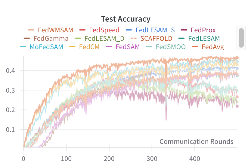
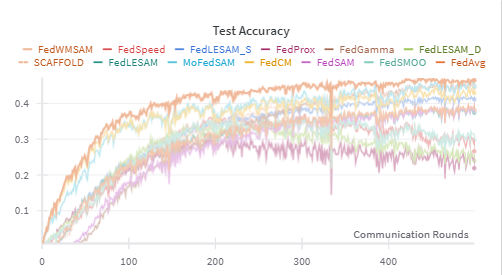
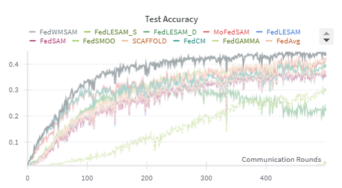
In this section, we present a detailed analysis of the experimental results, accompanied by visualizations to compare the performance of our proposed FedWMSAM method against several state-ofthe-art approaches.

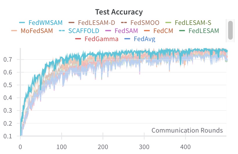
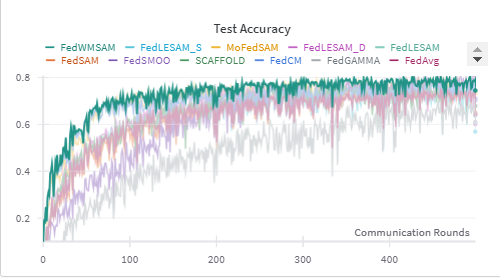
We begin by presenting the results on CIFAR-10, as shown in Figures 14 and15. The blue and green lines represent the FedWMSAM method, which demonstrates superior performance, with faster convergence and higher accuracy than other methods. The experiments were conducted with Dirichlet distribution parameters β = 0.1 and pathological heterogeneity γ = 3. This analysis highlights the effectiveness of FedWMSAM, particularly under heterogeneous conditions, and demonstrates its ability to achieve faster convergence and superior accuracy compared to alternative methods across a range of datasets.

S and greater heterogeneity). Under stronger non-IID conditions, our improvements become more significant, indicating that alignment, rather than sheer capacity, drives these enhancements.To demonstrate the adaptability of our method to the heterogeneity of real-world data, we conducted experiments on the OfficeHome dataset. As shown in Table2, FedWMSAM is best on 3/4 domains (Art/Clipart/Product) and achieves the best average, slightly trailing SCAFFOLD on Real-World. This suggests that aligning local updates to a global direction transfers across domains, complementing variance-reduction methods under specific domains.

S and greater heterogeneity). Under stronger non-IID conditions, our improvements become more significant, indicating that alignment, rather than sheer capacity, drives these enhancements.To demonstrate the adaptability of our method to the heterogeneity of real-world data, we conducted experiments on the OfficeHome dataset. As shown in Table2

S and greater heterogeneity). Under stronger non-IID conditions, our improvements become more significant, indicating that alignment, rather than sheer capacity, drives these enhancements.To demonstrate the adaptability of our method to the heterogeneity of real-world data, we conducted experiments on the OfficeHome dataset. As shown in Table

S and greater heterogeneity). Under stronger non-IID conditions, our improvements become more significant, indicating that alignment, rather than sheer capacity, drives these enhancements.