Waveform-Based Probabilistic Seismic Hazard Analysis Using Ground-Motion Generative Models

Within this framework, numerous studies have been conducted on each of its major components, including seismic source characterization (SSC; e.g., Field et al. (2014); Morikawa and Fujiwara (2016); Papadopoulos et al. (2021)), ground-motion characterization (GMC; e.g., Morikawa and Fujiwara (2013); Bozorgnia et al. (2014); Abrahamson et al. (2018)), and aleatory variability and epistemic uncertainty (e.g., Senior Seismic Hazard Analysis Committee (SSHAC) Florez et al. (2022). Florez et al. (2022) developed a cGAN model based on the Wasserstein GAN (WGAN) framework (Gulrajani et al., 2017), which we hereafter refer to as the conditional Wasserstein GAN-based GMGM (CW-GMGM). As the third GMGM, we develop a model by modifying the S-GMGM into a cGAN framework, utilizing a DNN architecture similar to that of Florez et al. (2022). This model is referred to as the conditional StyleGAN-based GMGM (CS-GMGM). These three GMGMs are trained on the same dataset based on the strong-motion observed records in Japan compiled in our previous study (Matsumoto et al., 2024), and their performance is evaluated by checking the waveforms as well as the distributions of generated data. We also propose a method for objectively determining the optimal number of training epochs based on quantitative evaluation metrics. Then, numerical experiments of PSHA using the trained three GMGMs are conducted. We demonstrate that the proposed methods can represent the seismic hazard as a set of ground-motion waveforms, and the hazard curves of IMs calculated from the evaluated waveforms are consistent with those of the PSHA results based on conventional GMMs. Furthermore, to demonstrate the engineering applicability of the proposed PSHA framework, we perform nonlinear dynamic response analyses of a building inputting ground-motion waveforms evaluated through the proposed method. In addition to demonstrating that the exceedance probabilities of EDPs can be evaluated in a straightforward manner, by applying hazard disaggregation (Bazzurro and Cornell, 1999) to the hazard curves of the EDPs, we show that the relationship between the EDPs and the seismic sources can be clearly analyzed.

In this section, we first present the proposed waveform-based PSHA formulation for evaluating the distribution of ground-motion waveforms. We then describe the computational methods used to perform the integration in waveformbased PSHA. Furthermore, we demonstrate a method for calculating the exceedance probabilities of IMs from the hazard analysis results.

In conventional PSHA, seismic hazard is expressed in terms of exceedance probability. However, defining the exceedance probability of ground-motion waveforms is challenging, as the target level for exceedance cannot be clearly specified. We propose to evaluate the seismic hazard in the form of probability distribution of ground-motion waveforms as follows:

in which g ∈ R M ×L is an M -component ground-motion waveform with L sampled time steps. m, r, and s are vectorvalued random variables representing information regarding source, path, and site, respectively. In conventional PSHA, magnitude and distance are used as the source and path characteristics, respectively. Here, to provide a more general formulation, we define m and r as vectors of random variables that include multiple attributes to be considered, for example, m = [magnitude, hypocenter coordinates, focal mechanism]. Although the feasibility of actually modeling such probability distributions is uncertain, this issue is not considered here, as the focus is on presenting a generalized formulation.

In equation 1, the probability distribution p(g | s) represents the distribution of ground-motion waveforms at a site of interest. The vector of random variables s is assumed to include not only site characteristics such as V S30 , but also deterministic information such as the geographic location of the site. Accordingly, p(m | s) represents the seismicity around the site, and p(r | m, s) represents information related to attenuation properties and geographic relationships between the sources and the site. The term p(g | m, r, s) represents the distribution of ground-motion waveforms conditioned on the source, path, and site characteristics. This can be modeled by constructing a GMGM whose conditional labels include m, r, and s. It should be noted that a GMGM is not the only possible approach; for example, simulation-based models capable of representing ground-motion variability could also be employed, but such considerations are left for future work. Based on this setting, a set of ground-motion waveforms following the distribution p(g | s) can be interpreted as representing the seismic hazard at the site of interest.

When using GMGMs to evaluate the distribution p(g | m, r, s), it is generally possible to obtain samples that follow this distribution, but not to evaluate the probability density p(g | m, r, s) itself. Therefore, the analytical evaluation of equation ( 1) is intractable, and equation (1) is evaluated using Monte Carlo integration (Assatourians and Atkinson, 2013).

Algorithm 1 presents the details of the Monte Carlo integration of the proposed method. The overall flow of the Monte Carlo simulation (MCS) is presented here, whereas more specific formulations for practical applications are described in the Numerical experiments section for each problem setting. The MCS is generally performed in three steps. The first step is the generation of an earthquake catalog for given source geometries and seismicity parameters. In this step, to provide a more general formulation, not only the stationary Poisson distribution but also time-dependent Algorithm 1 Sampling ground-motion waveforms based on equation (1) Require: Time period t; number of seismic sources N s ; target site condition s * ; target number of waveforms N w ;

generator G (joint or conditional); distance metric d(•, •); tolerance ϵ; and earthquake occurrence models for each source. Ensure: Set of ground-motion waveforms G wav ; total number of Monte Carlo cycles c sim ; cumulative event counts (c i ) Ns i=1 , in which c i is the total number of earthquakes from source i across all Monte Carlo cycles. Ensure: Ground-motion waveform g i,j,k ∈ G wav , denoting the k-th waveform from source i in Monte Carlo cycle j;

at generation time j = c sim and k

Sample the event counter s i for source i from its occurrence model 8:

earthquake occurrence models such as the Brownian passage time (BPT) distribution (Matthews et al., 2002) are considered. Therefore, seismic hazard is evaluated directly over a time period of t years, rather than as an annualized hazard. For each seismic source E i (i = 1, • • • , N s ), the number of earthquake occurrences s i within the t-year period is simulated based on the specified earthquake occurrence model. Subsequently, s i samples are drawn from the distribution p(m | s * ) for the given site condition s * , and an earthquake catalog is constructed.

The second step is the sampling of r. Based on the sampled source characteristics m * and given site condition s * , a sample following the distribution p(r | m, s) is obtained. Here, we assumed that samples can be drawn from the distributions p(m | s) and p(r | m, s). Such an assumption is common in probabilistic modeling and, as shown in the Numerical experiments section, also holds in practical implementations of PSHA.

The final step is the sampling of ground-motion waveforms based on the sampled m * , r * , and the given site condition s * . In the case of the GMGMs based on GANs, sampling is performed through the generator of the GAN. Let the generators of the S-GMGM, CW-GMGM, and CS-GMGM be denoted as G s , G cw , and G cs , respectively. For the S-GMGM, which models the joint distribution, a noise vector z ∼ p Z (z) is used as the input to generate data as follows:

in which y is the conditional labels and is a vector containing m, r, and s. Although the generator in a GAN is a deterministic function, it is trained as a mapping function that transforms the prior distribution p Z (z) into the data distribution. Therefore, the distribution of the generated samples follows a distribution approximates the distribution of the observed records. The conditional distribution is evaluated using rejection sampling (Tavaré et al., 1997), as described in Matsumoto et al. (2024):

ϵ > 0 is a tolerance. In practice, a sample that follows the conditional distribution is obtained by repeatedly generating ground-motion waveforms using equation ( 2) until the condition d(y, y * ) ≤ ϵ is satisfied.

For the CW-GMGM and CS-GMGM, the ground-motion waveforms are generated using the noise vector z and conditional label y as inputs:

As in the case of the S-GMGM, the distribution of the noise vector is transformed into the data distribution through the generator, and the ground-motion waveforms generated by equation 4 follow the distribution p(g | m, r, s).

Accordingly, in the CW-GMGM and CS-GMGM, a ground-motion waveform following the conditional distribution p(g | m, r, s) can be obtained simply by sampling one noise vector and inputting it into the generator together with m * , r * , and s * .

The above three steps are repeated until the target number of ground-motion waveforms, N w , is obtained. To maintain consistency among the sampled conditions, the MCS is not terminated immediately when c = N w , but rather after completing the entire MCS cycle in which c = N w is reached. Consequently, the total number of sampled groundmotion waveforms does not necessarily equal N w , and it holds that |G wav | ≥ N w . The resulting set of ground-motion waveforms:

represents an ensemble of ground-motion waveforms following the distribution p(g | s) in equation 1. The groundmotion waveforms with the same subscript i represent the waveforms associated with source i. The subscript k indicates the MCS cycle in which each waveform was obtained. The number of waveforms g i,j,k with the same subscripts i and k corresponds to the number of earthquakes that occurred from the source i during the k-th MCS cycle. By keeping track of the number of MCS cycles c sim , weighting information that accounts for the earthquake occurrence probability associated with each waveform is also retained. For example, the earthquake occurrence rate ν i of the source i over the t-year period can be evaluated as:

in which c i is the total number of earthquakes from the source i. These three quantities, G wav , c sim , and c i , together provide the basis for the waveform-based PSHA proposed in this study.

Hazard curves for IMs can be computed from the sampled waveforms G wav . Let IM i,j,k be the IM calculated from the ground-motion waveform g i,j,k ∈ G wav , and let P i (IM > x; t) be the t-year exceedance probability that the IM exceeds an intensity level x for source i We assume that {IM i,j,k } csim k=1 are independent and identically distributed (i.i.d.) across k. The estimator Pi (IM > x; t) for P i (IM > x; t) can be obtained as:

in which J i (k) is the set of indices j corresponding to waveforms with the same subscripts i and k. Since we consider both the Poisson and time-dependent earthquake occurrence models here, the t-year exceedance probability P (IM > x; t) for all target sources can be computed using the complementary event formulation as:

in which P (IM > x; t) is the estimator for P (IM > x; t). The coefficient of variation (COV) is a widely used metric for evaluating the uncertainty of exceedance probability estimates obtained from MCS (e.g., Au and Beck (2003); Houng and Ceferino (2025)). It is well known that MCS estimator P (IM > x; t) is unbiased, and its expectation is given by:

Therefore, the COV is calculated as:

In the numerical experiments conducted in this study, the true value of P (IM > x; t) cannot be evaluated. Therefore, equation ( 11) is evaluated by using the value of P (IM > x; t) instead.

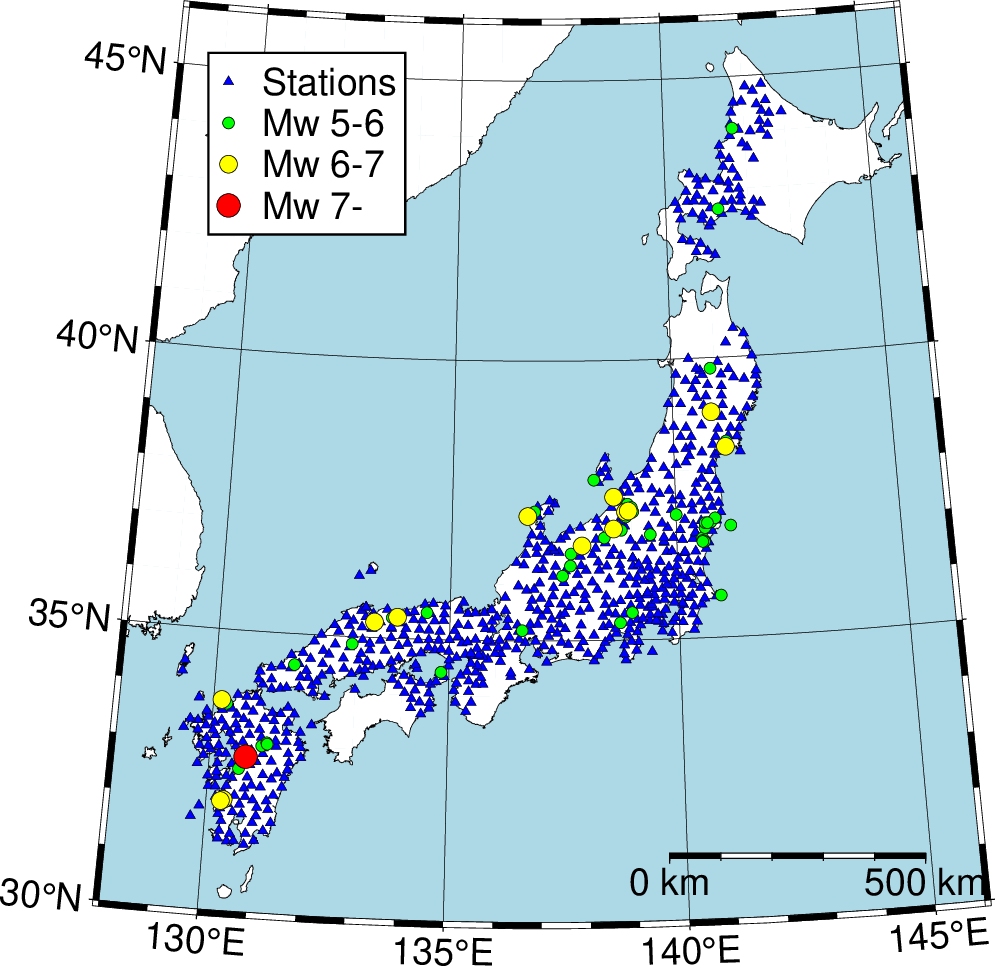
For training the three GMGMs (S-GMGM, CW-GMGM, and CS-GMGM), we use the dataset of crustal earthquakes in Japan compiled in our previous studies (Matsumoto et al. (2023) R RUP was calculated as the shortest distance from the rupture area to the station. When M W was sufficiently small that the earthquake could be considered a point source, R RUP was calculated as the hypocentral distance. The two horizontal components of ground motions were treated independently. To increase the amount of training data, the ground-motion time histories were rotated in the horizontal plane at 45-degrees intervals, and the separated components were used after removing duplicates. As a result, a total of 21,696 one-component horizontal ground-motion waveforms from 62 earthquakes were obtained. As a proxy for site characteristics, V S20 was calculated from the P-S logging results provided in the K-NET database, and V S30 was then estimated using the empirical formula proposed by Kanno et al. (2006):

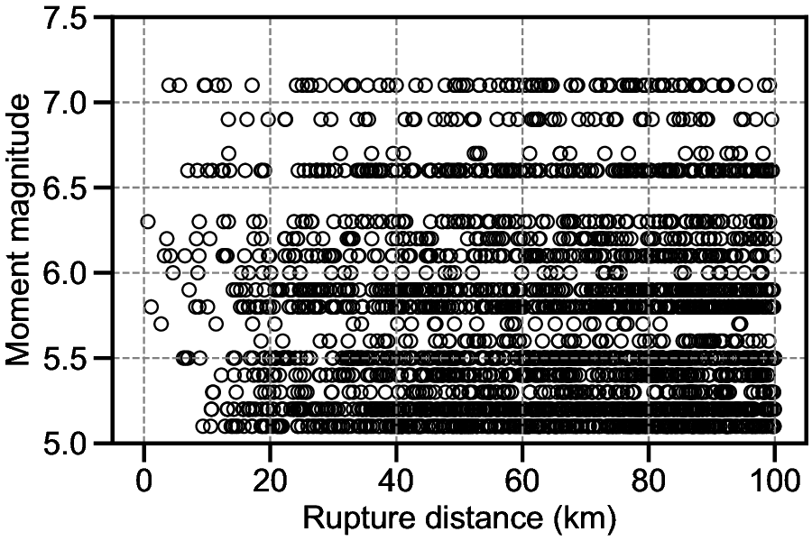
The locations of the earthquake epicenters and stations are shown in Figure 1, and magnitude-distance distribution is shown in Figure 2. Further details on the training dataset are provided in Matsumoto et al. (2023) and Matsumoto et al. (2024).

Several preprocessing steps were applied to the ground-motion waveforms. Each record was aligned with respect to the P-wave arrival time, and signals caused by aftershocks were removed by visually inspecting the waveforms. The S-GMGM and CS-GMGM (Matsumoto et al., 2024) were modeled using ground-motion data with a length of L = 8192 time steps, whereas the CW-GMGM (Florez et al., 2022) used data with a length of L = 4000. For each case, the end of the record was truncated, a cosine taper was applied to the final 100 steps, and 100 zeros were appended to both the beginning and the end of the record to match the required data length. The sampling frequency was kept at 100 Hz, and no bandpass filter was applied. Each waveform amplitude was normalized by its PGA, and the PGA value was included as one of the conditional label elements. Accordingly, the conditional label is defined as the four-dimensional vector y = [M W , R RUP , V S30 , PGA] T , in which the natural logarithm is applied to R RUP , and the base-10 logarithm to V S30 and PGA. Finally, each component of y was normalized so that the mean and standard deviation across the entire dataset were 0 and 0.1, respectively.

An overview of the DNN architectures of the S-GMGM, CW-GMGM, and CS-GMGM is shown in Figure 3. The DNN architecture of Matsumoto et al. (2024) was employed for the S-GMGM, with only the dimensionality of the conditional label modified. The generator of the S-GMGM takes a noise vector z ∈ R 512 as input and generates a ground-motion waveform g ∈ R 1×8192 and its conditional label y ∈ R 4 . The discriminator takes both g and y as input and outputs a scalar value.

The CW-GMGM adopts the same DNN architecture as Florez et al. (2022). We constructed the DNN using the program code provided in their GitHub repository. The only modification was to the number of ground-motion components: while the original model handled three components, the CW-GMGM was adjusted to handle a single component by modifying the corresponding DNN parameters. The generator of the CW-GMGM takes a noise vector z ∈ R 100 and conditional label y ∈ R 4 as inputs and generates a ground-motion waveform g ∈ R 1×4000 . The discriminator takes both the g and y as input and outputs a scalar value. Although the discriminator in a WGAN is generally referred to as a critic, it is referred to as a discriminator in this study for consistency.

The CS-GMGM was constructed by modifying the generator of the S-GMGM into a cGAN framework. Following Florez et al. (2022), the conditional labels were embedded and concatenated with the noise vector before being input into the generator. The discriminator architecture was identical to that of the S-GMGM. The generator takes a noise vector z ∈ R 512 and conditional label y ∈ R 4 as inputs and generates a ground-motion waveform g ∈ R 1×8192 , while the discriminator takes g and y as inputs and outputs a scalar value.

The theoretical background of these GAN models can be found in Florez et al. (2022) and Matsumoto et al. (2024), and more detailed DNN configurations are available in our GitHub repository.

The hyperparameters for the S-GMGM and CS-GMGM were set to the same values as those used in Matsumoto et al. (2024). The learning rate was 0.002, the batch size was 64, and the dimensions of both the noise vector and the intermediate latent variable were 512. A standard normal distribution was used as the prior distribution of the noise vector. The Adam optimizer (Kingma and Ba, 2017) was used for training.

For the CW-GMGM, several models were initially trained by modifying the hyperparameters proposed in Florez et al. (2022), and their performance was compared. As a result, only the batch size and the number of training epochs were changed, while the other hyperparameters were kept the same as in Florez et al. (2022). The learning rate was set to 1 × 10 -4 , the batch size to 64, and the noise vector dimension to 100. A standard normal distribution was used as the prior distribution of the noise vector. The Adam optimizer (Kingma and Ba, 2017) was also used for training.

All deep learning processes and the construction of DNNs were implemented using the Python library PyTorch (Paszke et al., 2019). Additional details on the hyperparameter settings are available in our GitHub repository. The discriminator of the CS-GMGM has the same architecture as that of the S-GMGM.

Since the loss function of GANs depends on the training state of the discriminator, it is difficult to use the loss for relative comparison of the model performance across epochs. When applying GMGMs to PSHA, it is therefore necessary to establish an objective method for determining the optimal number of epochs. In this subsection, we extend the model evaluation method proposed by Matsumoto et al. (2023) and propose a new approach for relative performance evaluation across different epochs. The model performance is assessed based on how well the generator approximates the distribution of the training dataset. Let the training dataset be

and the set of ground-motion waveforms generated by the GMGM at epoch l as

Each ground-motion waveform is assumed to be an i.i.d. sample drawn from the probability distributions of the observed records p o and the generator p g,l , respectively. Using a feature vector ξ that characterizes the ground-motion waveform, the similarity between p o and p g,l is approximately evaluated by the Sinkhorn divergence (Cuturi (2013); Feydy et al. (2019)) as follows:

in which po and pg,l are empirical measures represented by the set of feature vectors ξ calculated from D o and D g,l , respectively. The term OT ϵ is defined as:

in which X is the data space, ϵ > 0 is the temperature parameter for entropy regularization, and C is the cost function.

We set C as follows:

The Sinkhorn divergence is an optimal transport-based metric that enables statistically stable and computationally efficient evaluation even for high-dimensional data. The value S ϵ ≥ 0 becomes zero when p o = p g,l , and smaller values indicate better approximation of the distribution. Accordingly, by selecting the elements of ξ based on the purpose of the GMGM development and evaluating the approximation accuracy of their joint distribution, the model performance at a given epoch can be quantitatively assessed. (Malhotra, 1999) s ξ3 log 10 (ξ3) Instrumental seismic intensity (Japan Meteorological Agency, 2025) -ξ4 ξ4 Predominant frequency (Rathje et al., 1998) Hz ξ5 ξ5 Zero-level crossing rate (Rezaeian and Der Kiureghian, 2008) /s ξ6 ξ6 Negative maxima and positive minima (Rezaeian and Der Kiureghian, 2010) /s ξ7 ξ7 Significant duration, D5-95 (Trifunac and Brady, 1975) s D5-95 D5-95 Significant duration, D5-45 (Rezaeian and Der Kiureghian, 2010) s D5-45 D5-45 Arias intensity (Arias, 1970) cm/s IA log 10 (IA) Spectrum intensity (Housner, 1961) cm SI log 10 (SI) Mean period (Rathje et al., 1998) s Tm Tm

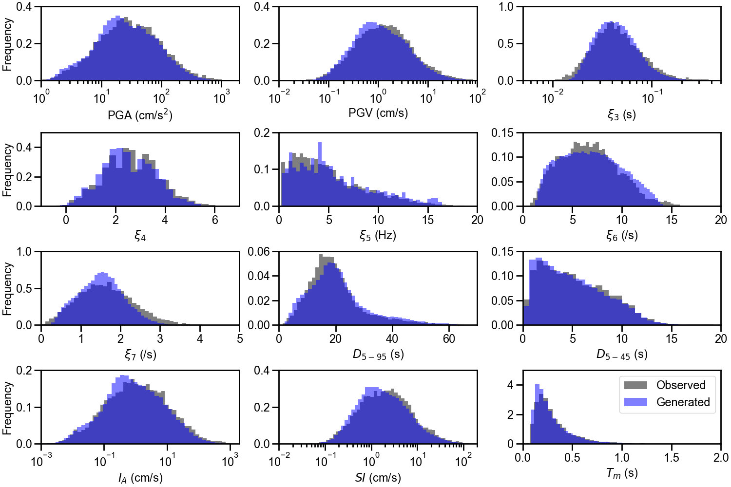
In this study, as an example, twelve indices that can be calculated from ground-motion waveforms were adopted as the elements of ξ. Table 1 shows the list of indices. These indices were selected to evaluate various characteristics of ground motions, including peak amplitude, power, duration, and frequency content. The specific definitions and calculation methods for each index are provided in Appendix A. The Sinkhorn divergence was computed using the Python library GeomLoss (Feydy et al., 2019), and details of the implementation are available in our GitHub repository.

We first evaluated the S-GMGM. The maximum number of training iterations was set to 100,000, and the generator parameters were saved every 100 iterations ( l = 100, 200, • • • , 100000), resulting in 1,000 models corresponding to different training states. Here, an iteration refers to a single completion of the training loop. Then, 100,000 random noise vectors z were sampled to generate the set D g,l and the corresponding set of conditional labels Y g,l . For both D o and D g,l , feature vectors {ξ

were computed. As shown in Table 1, several indices were transformed to the base-10 logarithmic scale, and each element was standardized using the mean and standard deviation of {ξ (o) i }. The similarity between distributions was then evaluated using equation ( 13). Among iterations with high similarity, we visually inspected the generated waveforms, spectra, and distributional characteristics following the procedure in Matsumoto et al. (2024), and finally selected the model at 35,300 iterations.

Next, the CW-GMGM and CS-GMGM were evaluated. To ensure consistent analysis conditions, the conditional labels Y g,l generated by the optimal S-GMGM were used for data generation. Thus, for both the CW-GMGM and CS-GMGM, N g = 100, 000. For the CW-GMGM, the maximum number of epochs was set to 1,000, and the model was saved every 10 epochs. For the CS-GMGM, the maximum number of iterations was set to 100,000, and the model was saved every 100 iterations. The same evaluation procedures as those used for the S-GMGM were applied, and the final models were selected at 250 epochs for the CW-GMGM and 42,900 iterations for the CS-GMGM.

In this subsection, we examine the generated results of the optimal GMGMs. Although verifying the performance of the GMGMs is important for their application to PSHA, a detailed examination is not the main focus of this paper. Therefore, only a portion of the generated results for the S-GMGM is presented in the main text, while additional results for the S-GMGM, as well as the results for the CW-GMGM and CS-GMGM, are provided in the supplemental material to this article.

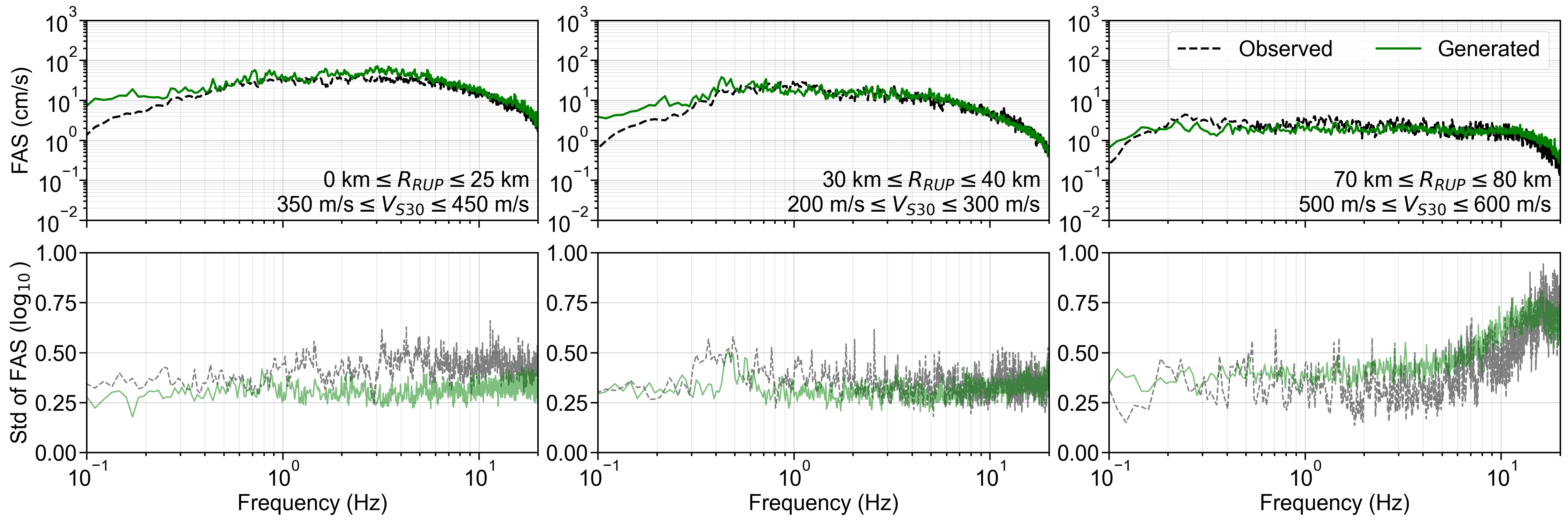
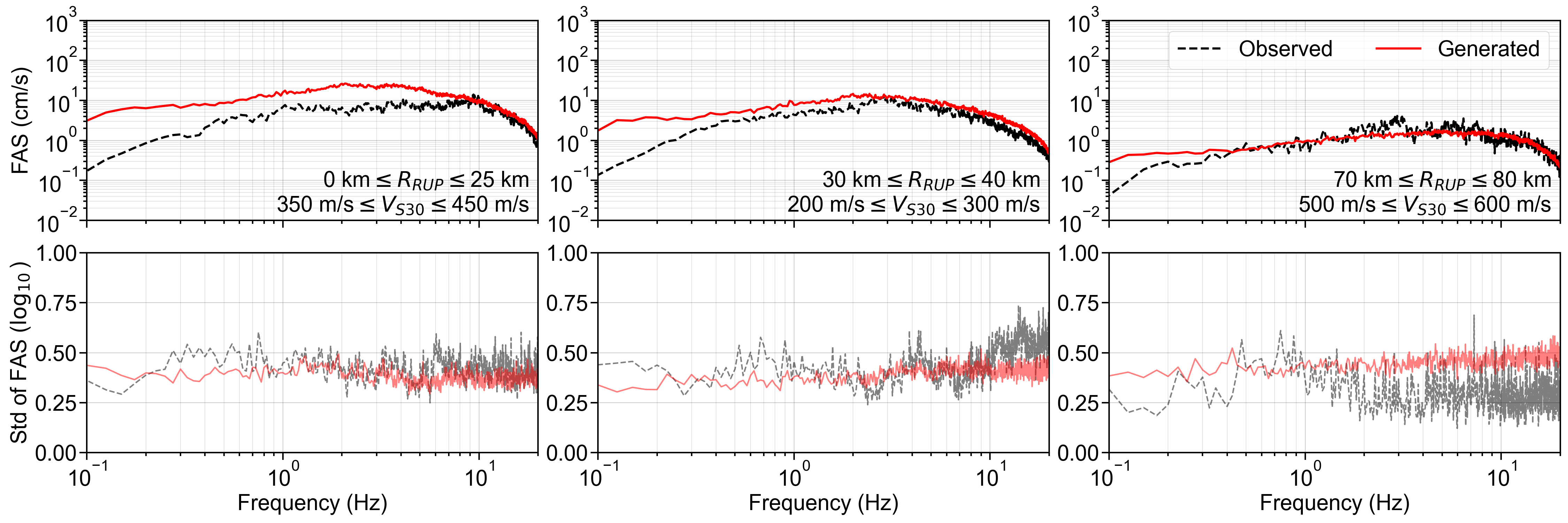
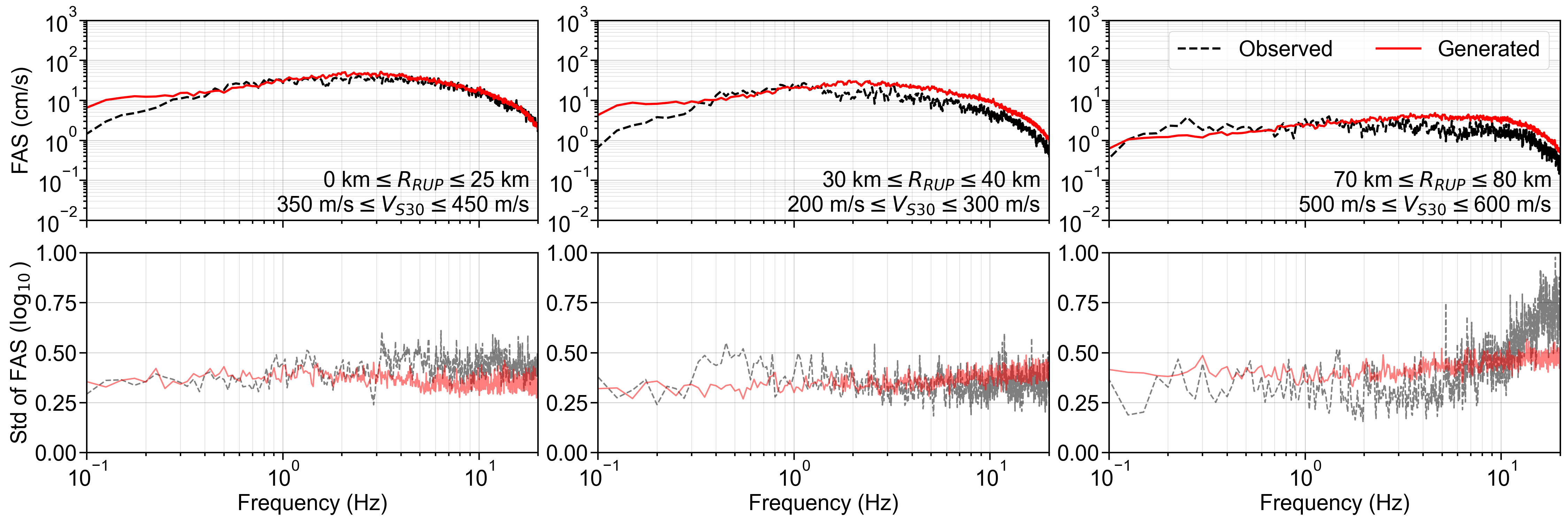
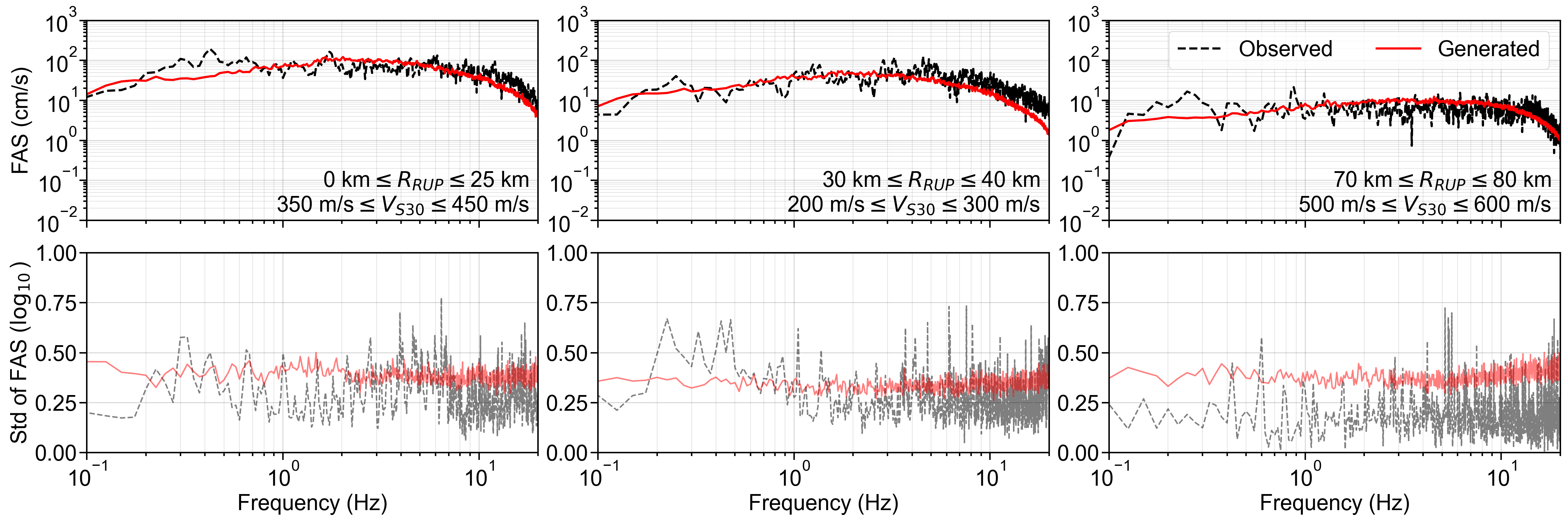
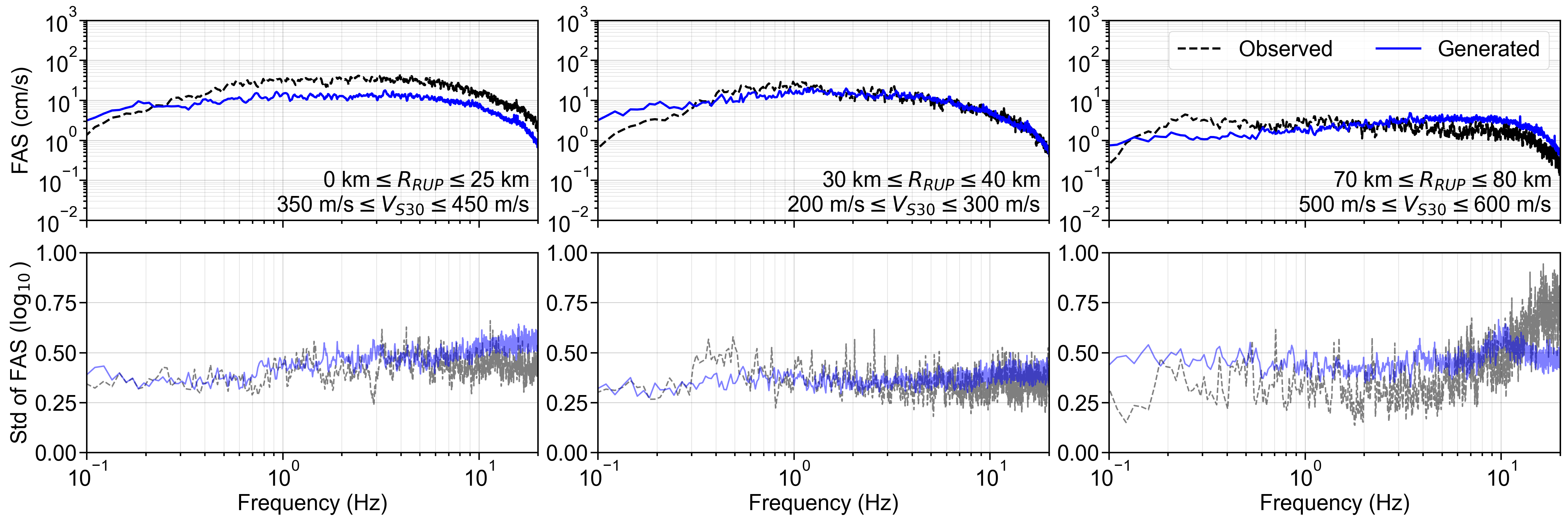
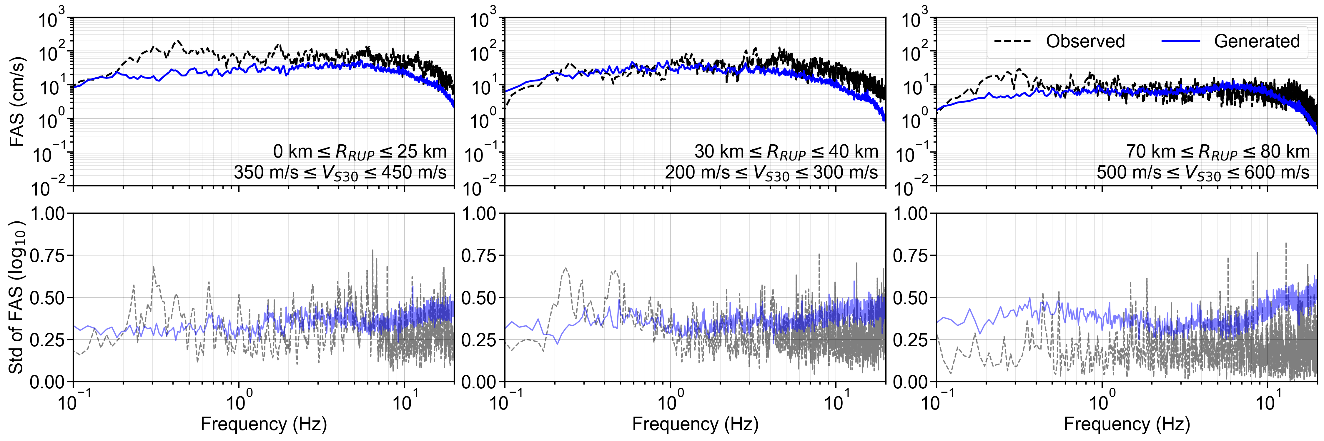
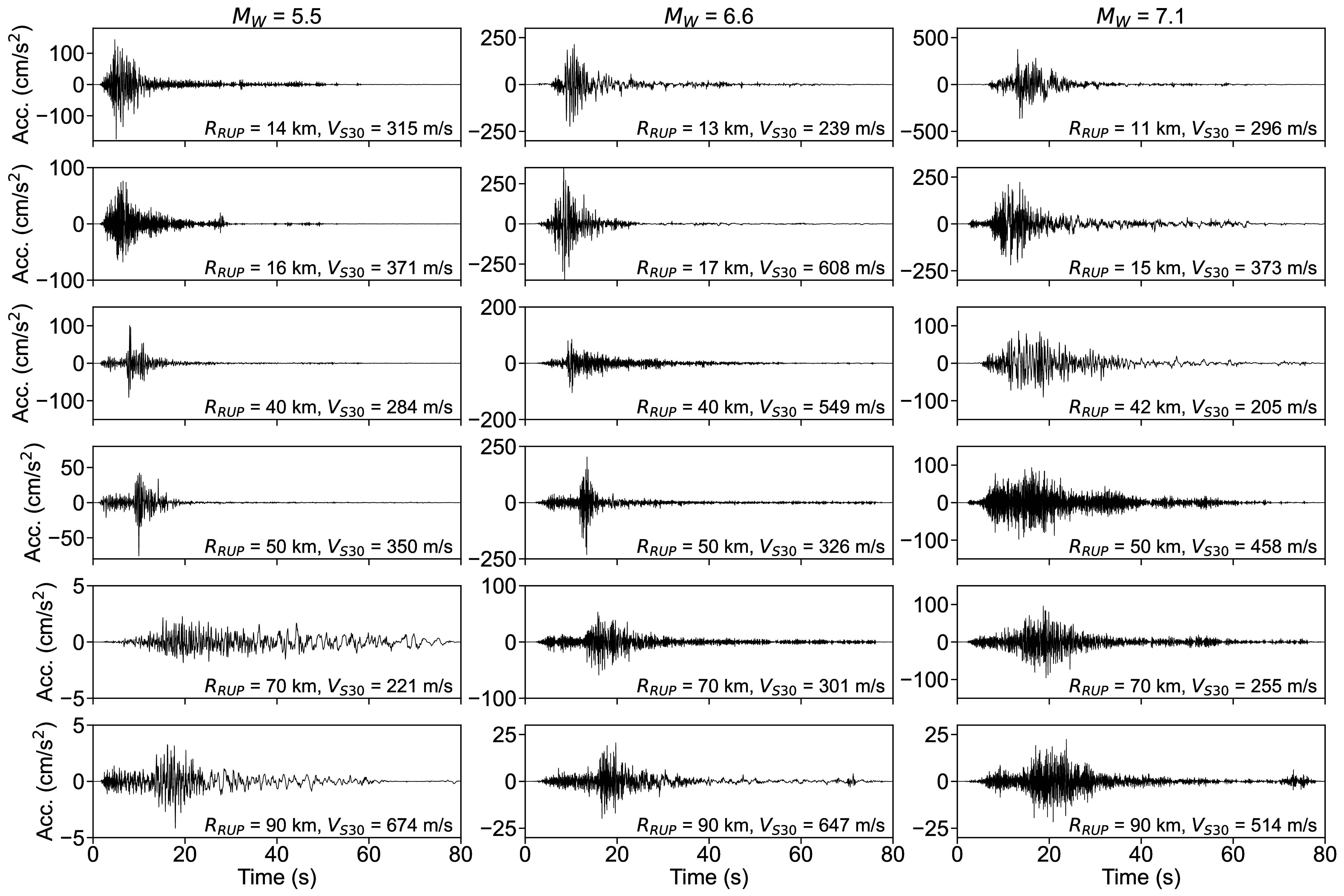
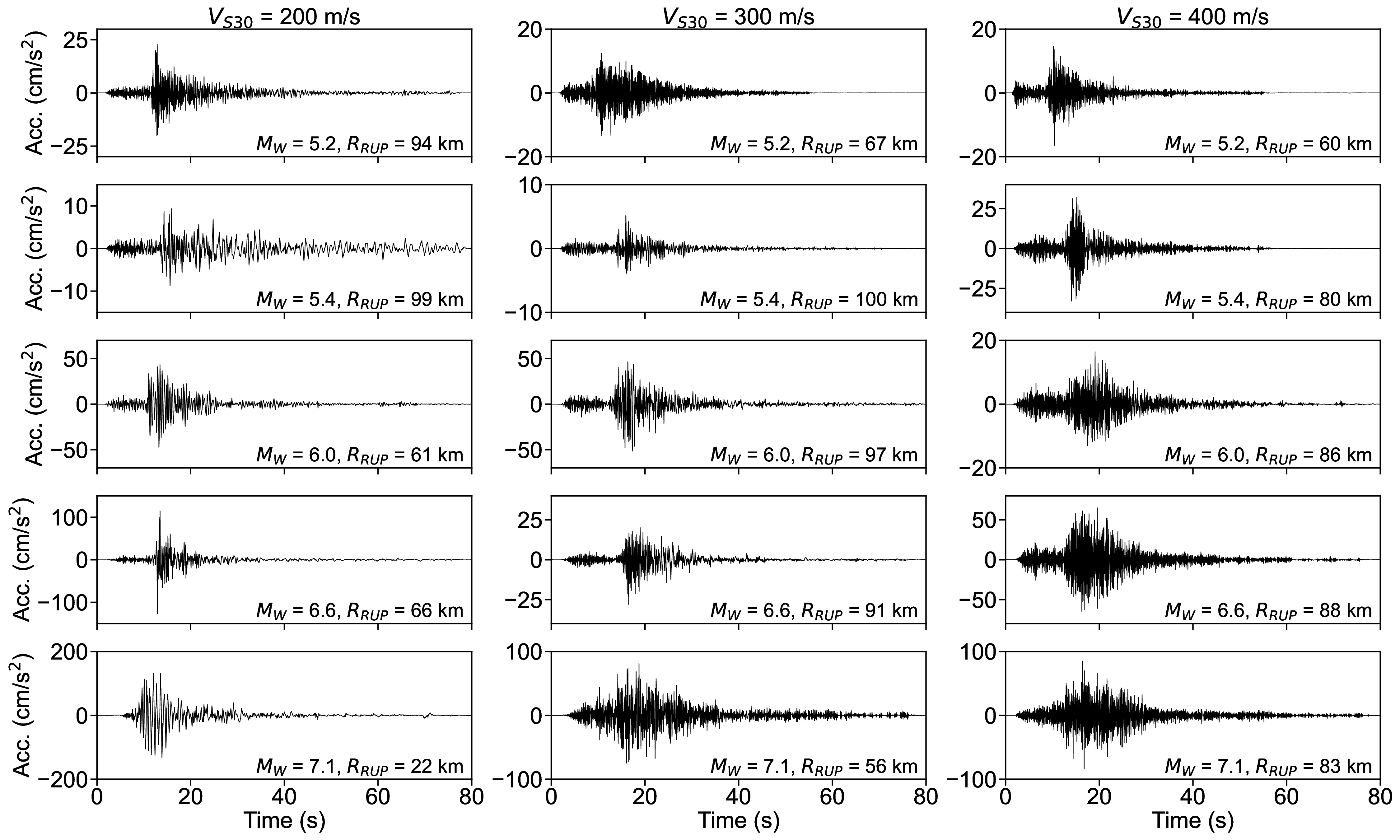
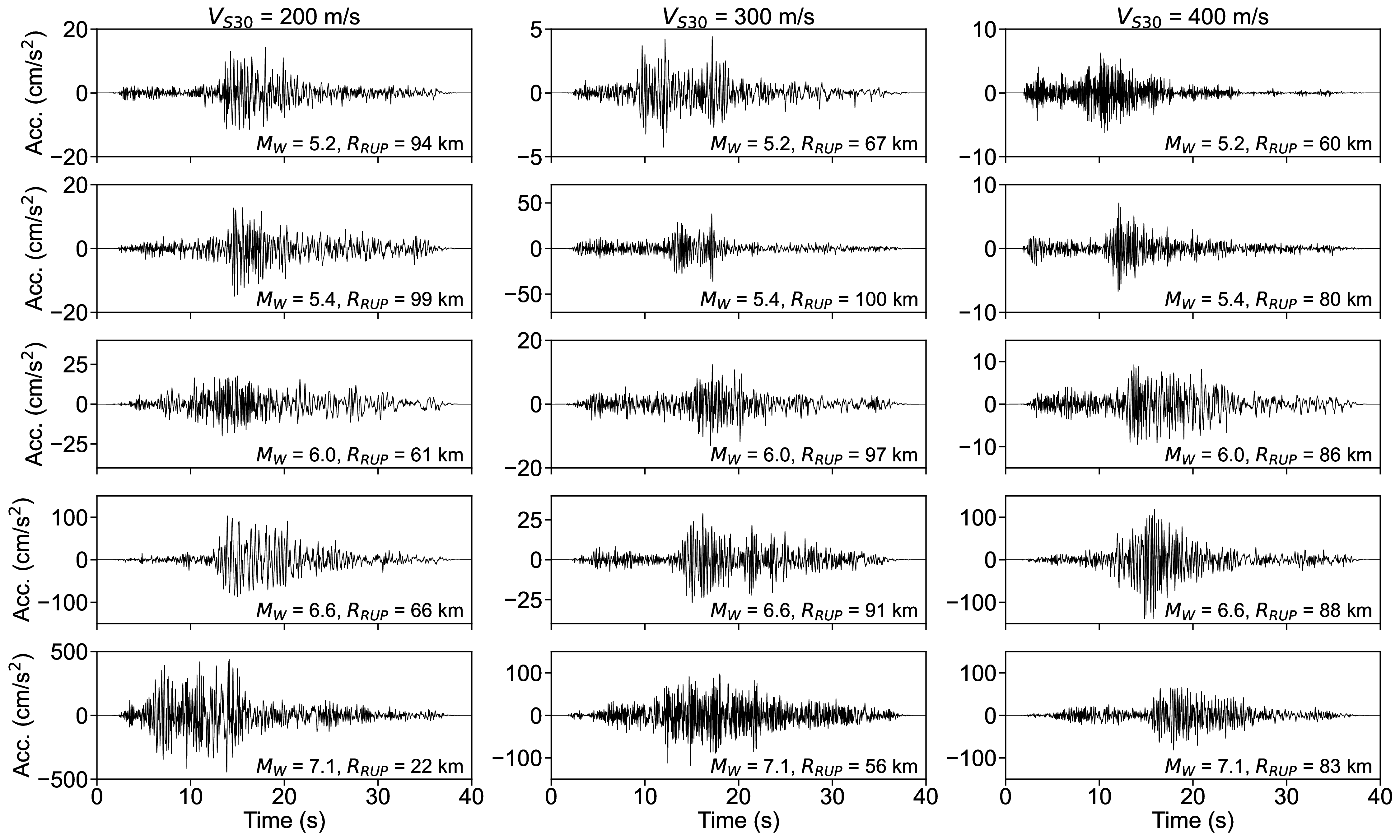
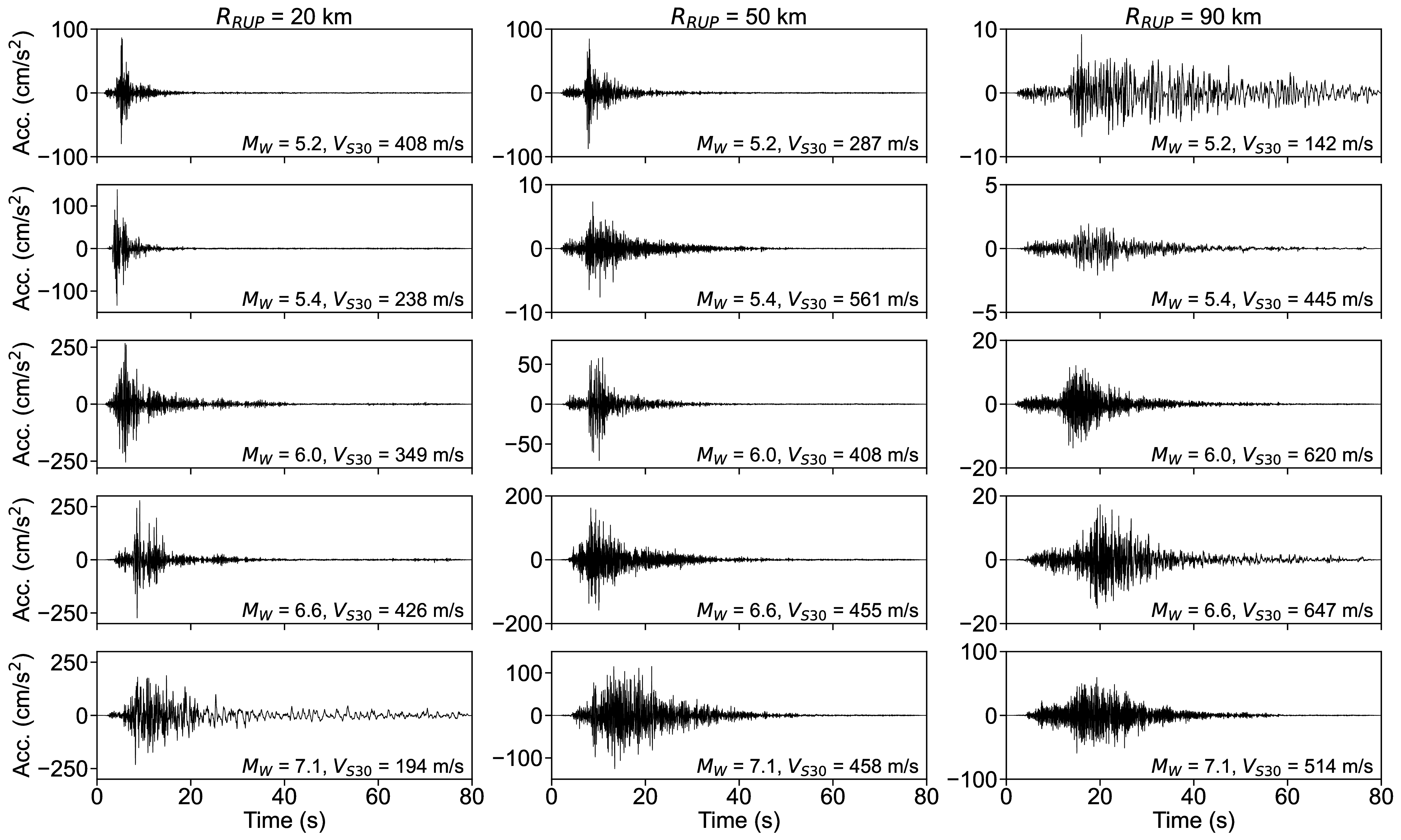
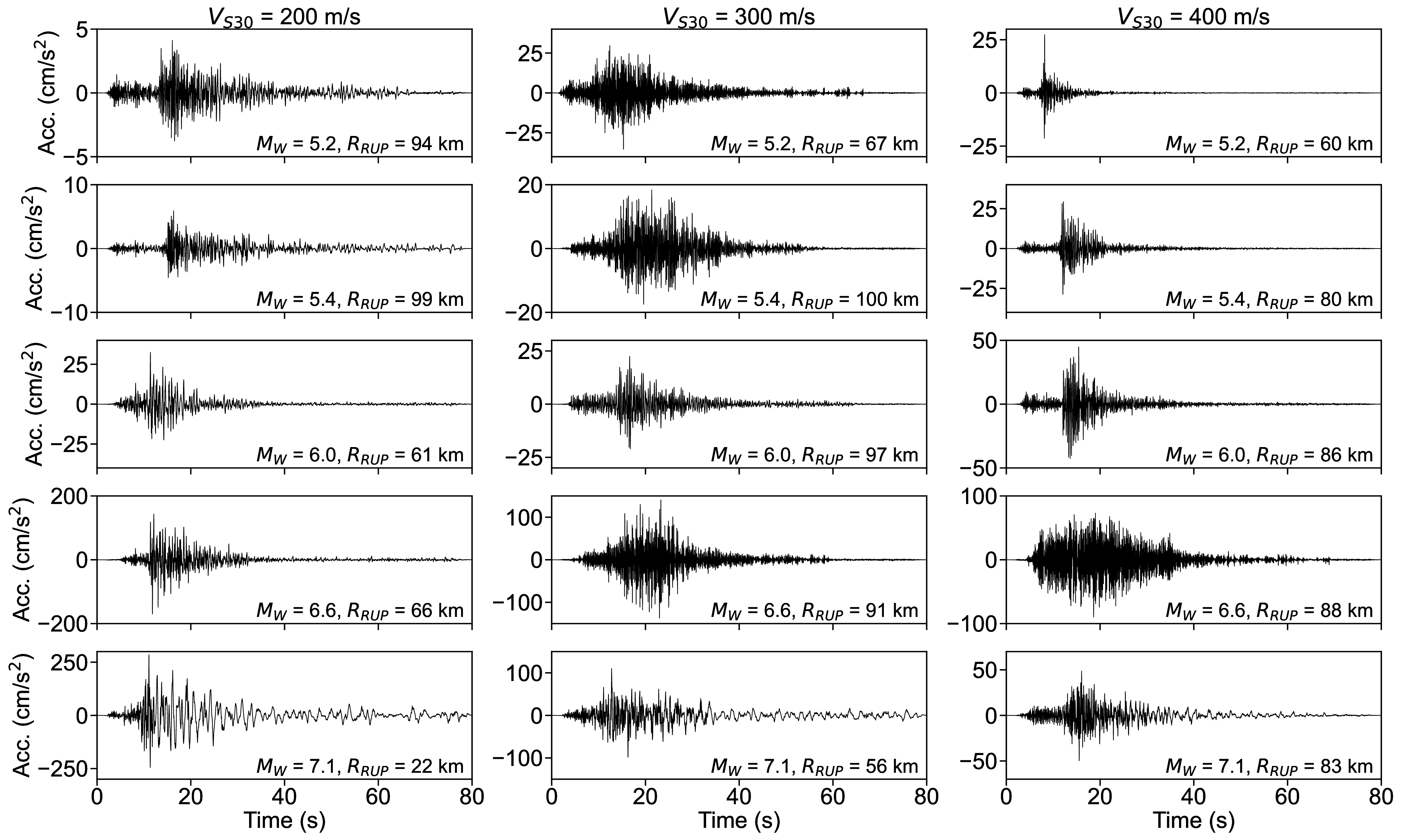
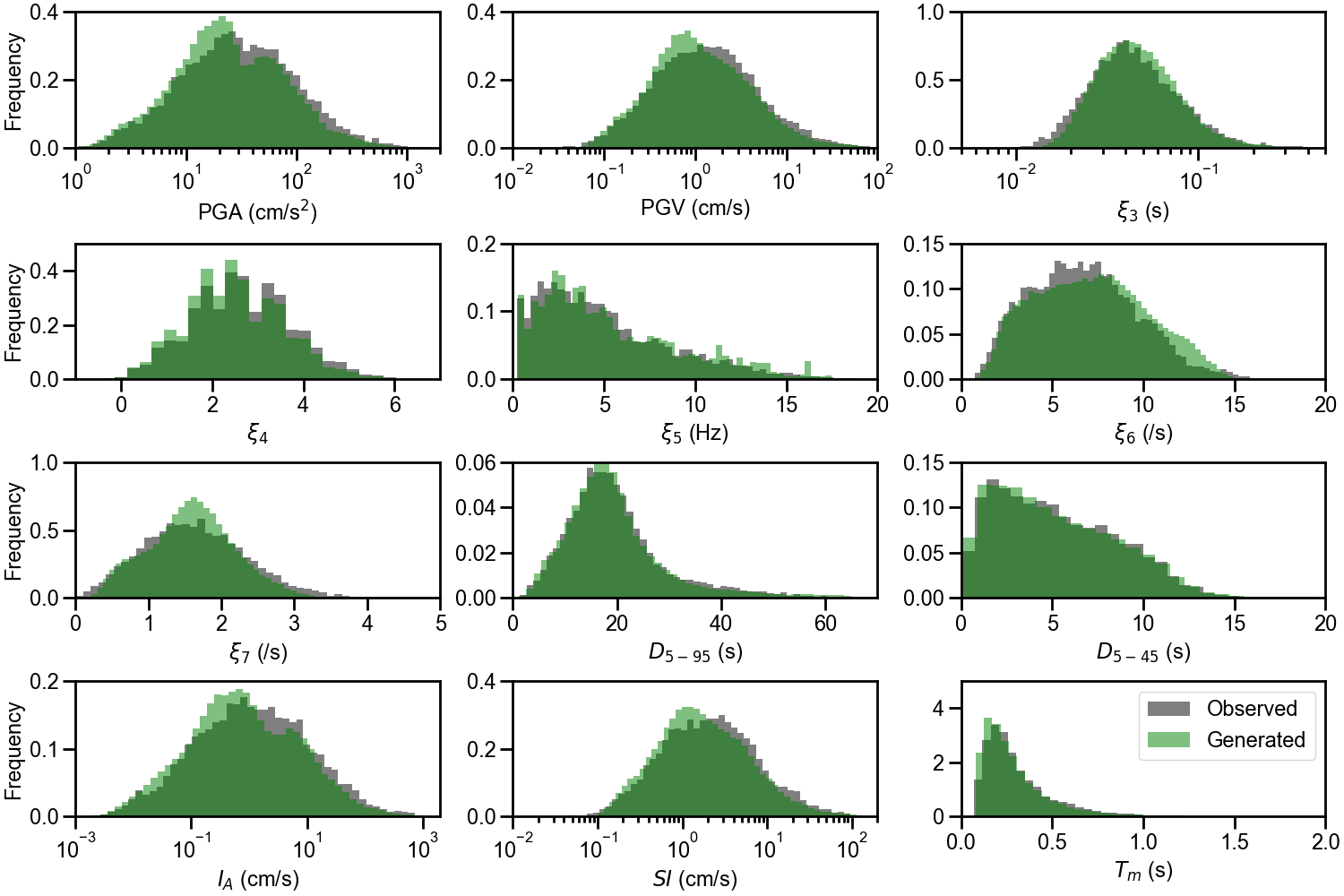
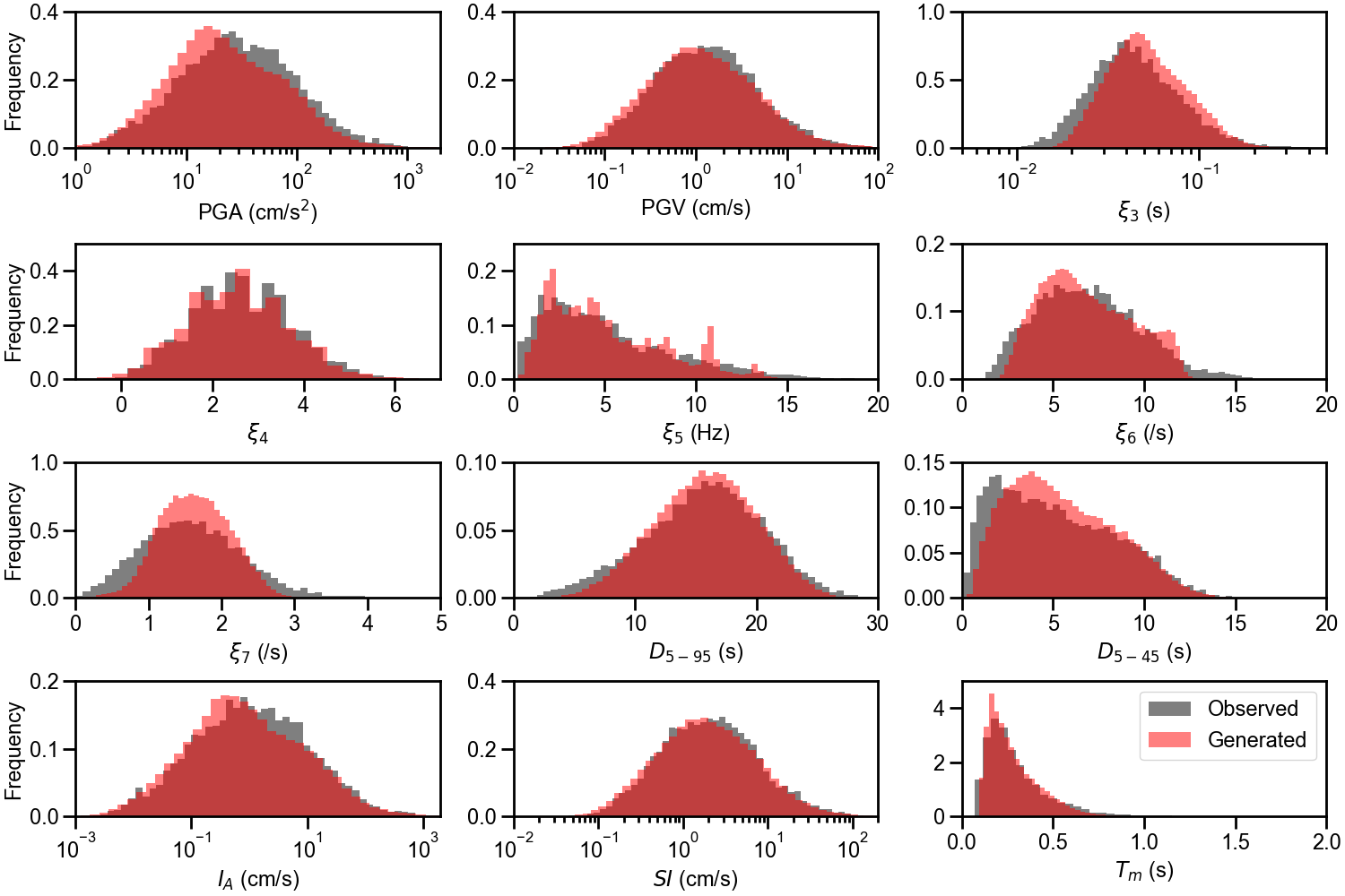
For the S-GMGM, 100,000 samples of z were drawn from a standard normal distribution, and 100,000 ground motions g and their corresponding conditional labels y were generated. Several post-processing steps were applied to the ground motions. After removing the offset so that the mean acceleration becomes zero, a fourth-order Butterworth filter was applied with a 0.1 Hz low-frequency cutoff and a 20 Hz high-frequency cutoff. A cosine taper was then applied to the first 100 steps and the last 200 steps of the waveform, and the amplitude was restored by multiplying the PGA contained in the corresponding conditional label. Examples of the acceleration waveforms with specific M W , R RUP , and V S30 scenarios are shown in Figure 4. Waveforms for different M W , R RUP , and V S30 scenarios are shown in Figures S1 andS2. Waveforms generated by the CW-GMGM and CS-GMGM using the same M W , R RUP , and V S30 scenarios are also shown in Figures S3 to S5 and Figures S6 to S8, respectively. The post-processing procedures for the waveforms are the same as those for the S-GMGM. The generated waveforms capture characteristics such as the onset of P and S waves, envelope shapes, and the magnitude and distance scaling. They also capture site effects, such as the appearance of long-period vibrations under relatively soft site conditions and short-period vibrations under relatively hard site conditions. Statistical comparisons of the Fourier amplitude spectra between the generated waveforms and the observed records are shown in Figures S9 to S11. Comparisons of the distributions of the ground-motion characteristic indices listed in Table 1 are shown in Figure 5 and Figures S12 to S13. The PGV values were computed by obtaining $FFFPV the velocity waveforms through numerical integration after removing the long-period components using a fourth-order Butterworth filter with a 0.2 Hz low-frequency cutoff. The SI values were calculated by computing the 5% damped velocity response spectra using the Nigam-Jennings method (Nigam and Jennings, 1969). As in the previous study (Matsumoto et al., 2024), it can be seen that the distributions of the generated waveforms are consistent with those of the observed records in terms of both temporal and frequency characteristics.

Next, for the 100,000 conditional labels generated by the S-GMGM, the relationships among the labels are compared in Figure 6. The distributions of the conditional labels are well matched with those of the observed records. In addition, Figures 6 (a) and (b) show the ranges of magnitude, distance, and V S30 that can be generated by the S-GMGM, and can be interpreted as figures indicating the applicability range for PSHA. It is difficult to evaluate the applicability of the cGAN-based models, CW-GMGM and CS-GMGM, to PSHA based on the range of their generated conditional labels, because these models require the conditional labels to be specified during data generation and do not learn the distribution of the labels themselves. One advantage of the S-GMGM is that its applicability to PSHA can be examined by checking the distribution of the generated data.

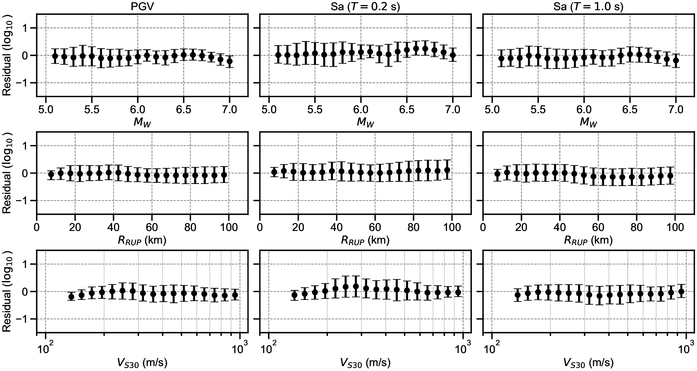
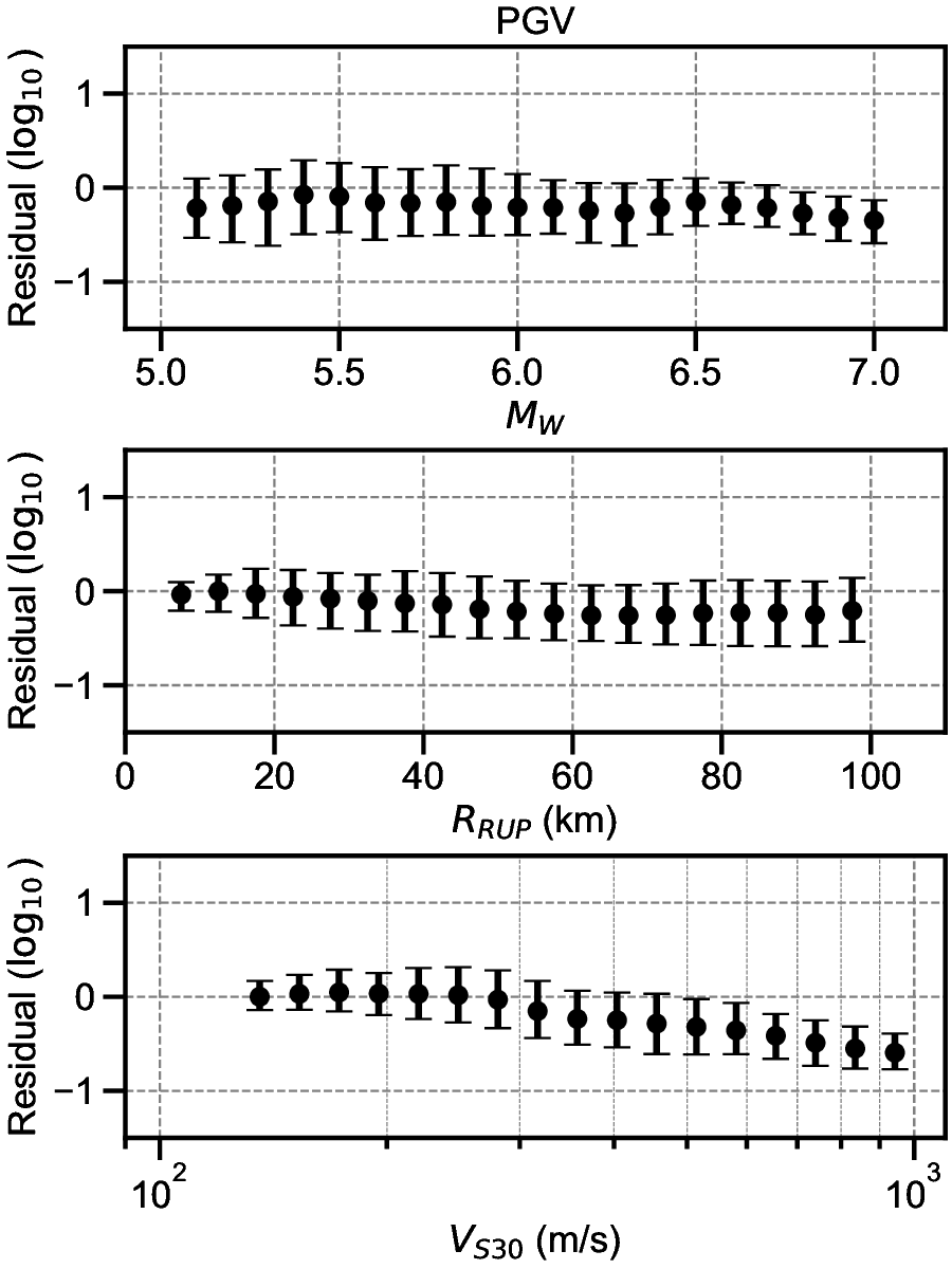
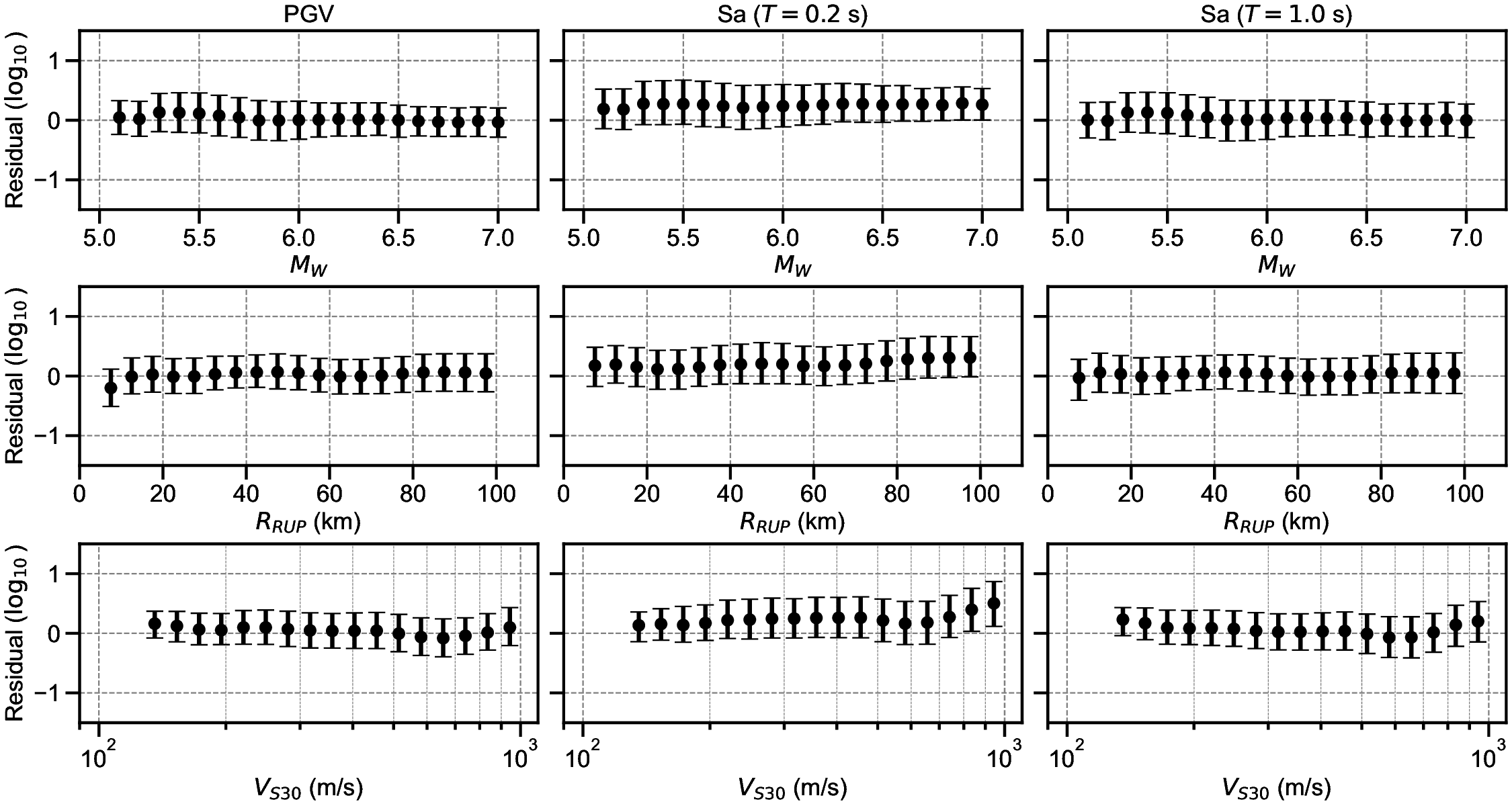
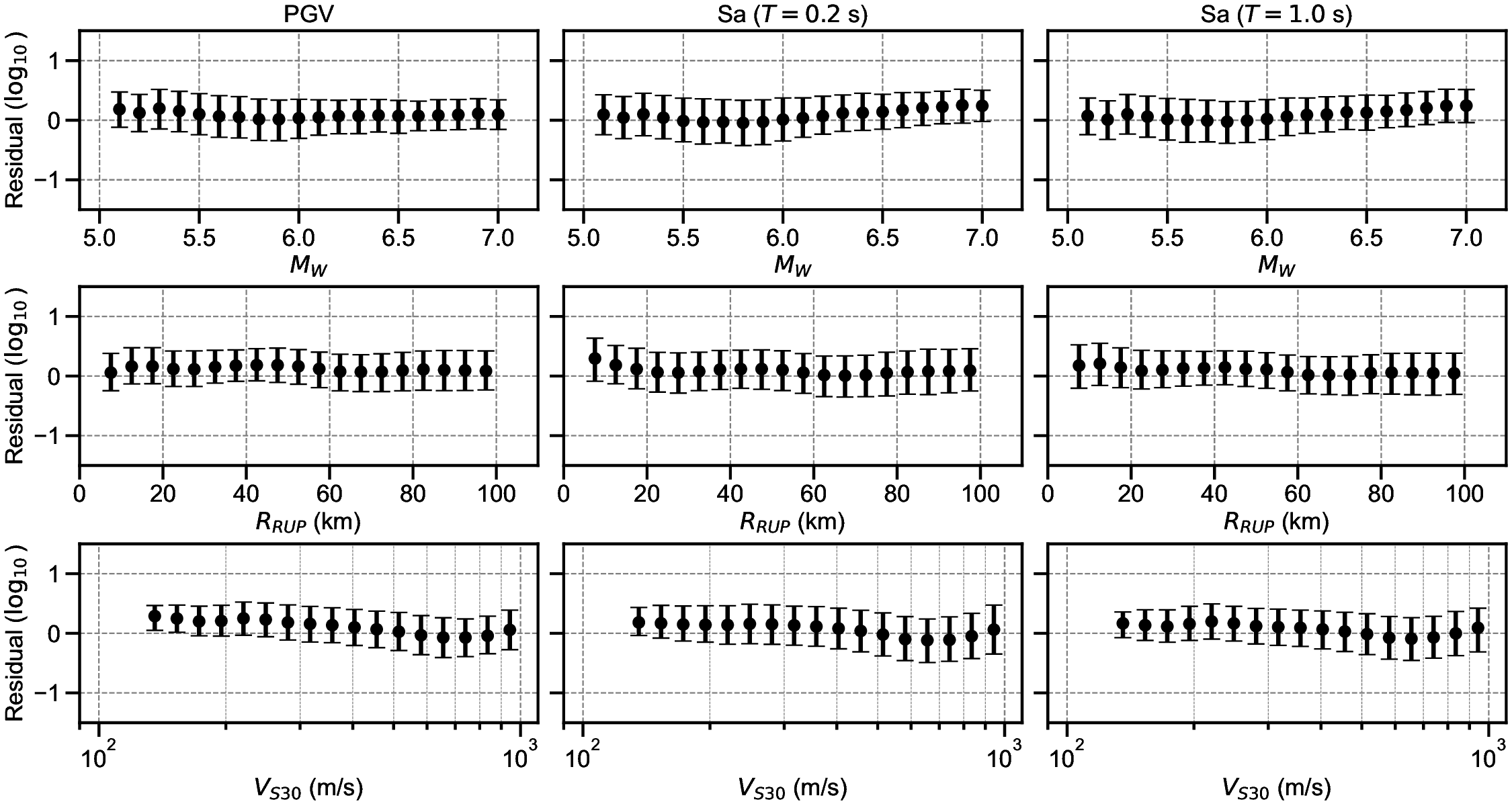
Finally, the residuals between the GMGMs and GMMs are compared for PGV and for the 5% damped spectral acceleration at natural periods of T = 0.2 s and T = 1.0 s. The residuals were defined as the base-10 logarithm of the GMGM divided by the GMM. The Si and Midorikawa (1999) (hereafter, SM99) GMM and the Morikawa and Fujiwara (2013) (hereafter, MF13) GMM, which are used in the development of the national seismic hazard map for Japan (Fujiwara et al., 2023), were employed, and four NGA West2 GMMs (Abrahamson et al. (2014), ASK14; Boore et al. (2014), BSSA14; Campbell and Bozorgnia (2014), CB14; Chiou and Youngs (2014), CY14) were also used for comparison. For each GMM, only the terms that can be computed using the M W , R RUP , and V S30 were employed. The specific formulations are presented in Appendix B. As the IM, the maximum amplitude of the two horizontal components was used in the SM99 GMM, RotD100 (Boore, 2010) was used in the MF13 GMM, and RotD50 (Boore, 2010) was used in the NGA West2 GMMs. Figure 7 shows the residual plots between the S-GMGM and the MF13 GMM. The residual plots between the S-GMGM and the other GMMs are shown in Figures S14 to S18, those for the CW-GMGM in Figures S19 to S24, and those for the CS-GMGM in Figures S25 to S30. Note that the GMGMs treat the two horizontal components independently, whereas the MF13 GMM uses RotD100, which leads to 1 between the observed records and ground motions generated by the S-GMGM.

an apparent underestimation. The analysis results are therefore qualitatively consistent when this modeling difference is taken into account. In addition, the median residual is approximately constant over a wide range of M W , R RUP , and V S30 , indicating that the magnitude and distance scaling, as well as the amplification effects of the surface soil, are appropriately represented.

We examine the proposed waveform-based PSHA using two numerical experiments. The first example considers a hypothetical single area source, whereas the second example focuses on an actual site and the surrounding faults in Japan. For each case, we present the set of waveforms sampled by Algorithm 1 and compare the resulting hazard estimates with those obtained from a conventional PSHA using GMMs to examine the validity of the proposed approach. The PSHA procedure based on GMMs follows the methodology described in Fujiwara et al. (2023). Following common settings in engineering applications (Gerstenberger et al., 2020), the seismic hazard is evaluated for a 50-year period in this study.

After presenting and examining the hazard analysis results, nonlinear dynamic response analyses are conducted for a five-degree-of-freedom (5DOF) building model using the ground-motion waveforms sampled in numerical example 2. Based on the building response time histories, the exceedance probabilities of the EDPs are evaluated. We also show the hazard deaggregation can be performed targeting EDPs with a straightforward manner. All analyses were performed using Python 3.12 on a Ryzen 9 9950X 16-Core Processor and 64 GB RAM. An NVIDIA RTX 4000 Ada GPU was used to generate the ground-motion waveforms with the GMGMs.

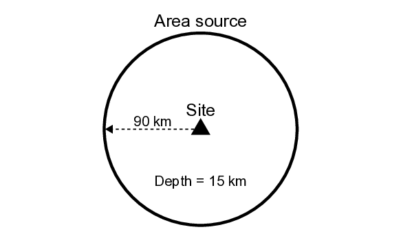
Figure 8 shows the setting of the target site and area source. A circular source with a radius of 90 km is defined on a horizontal plane located 15 km beneath the site. The value of V S30 at the site was set to 356 m/s. The earthquake occurrence model is assumed to follow a stationary Poisson process, with the minimum and maximum magnitudes set Earthquakes are assumed to occur uniformly within the source. Let r denote the horizontal distance from the center of the area source to the hypocenter. The probability density function p(r) is independent of magnitude and is given by:

in which R is the radius of the area source. The hypocentral distance r is computed as:

The probability density function p(m) for magnitude m is defined based on the Gutenberg-Richter (GR) law as a truncated exponential distribution with upper and lower bounds:

in which b is the b-value of the GR law, taken as 0.9 following Fujiwara et al. (2005).

Sampling from the distribution given in equations ( 16) and ( 18) was performed using inverse transform sampling (Bishop, 2006). Let u be a random variable uniformly distributed over the interval [0, 1]. Then the samples of r and m are obtained as:

Based on the above configuration, sampling of ground-motion waveforms was conducted using Algorithm 1. We set the number of sampling iterations to c sim = 20, 000, which resulted in 500,313 waveforms for the S-GMGM and 499,129 waveforms for the CW-GMGM and CS-GMGM. For the S-GMGM, the tolerances were set to 0.05 for M W , 5 km for R RUP , and 5 m/s for V S30 . The sampled ground motions were post-processed using the same procedure as described in Training results subsection. The sampling required approximately 2,586 min for the S-GMGM, about 2 min for the CW-GMGM, and about 10 min for the CS-GMGM. Because the computational cost of generating ground-motion waveforms is very low, the sampling for both the CW-GMGM and CS-GMGM took approximately 82 min and 20 min, respectively, when executed using only a CPU.

Figure 9 shows the hazard analysis results obtained using the S-GMGM. The results obtained using the CW-GMGM and CS-GMGM are presented in Figures S31 andS32, respectively. The sampled waveforms follow the assumed distributions p(r) and p(m), and the waveforms exhibit the expected trend of larger amplitudes at shorter distances and for larger magnitudes. These observations confirm that the seismic hazard is appropriately represented through the collection of sampled waveforms.

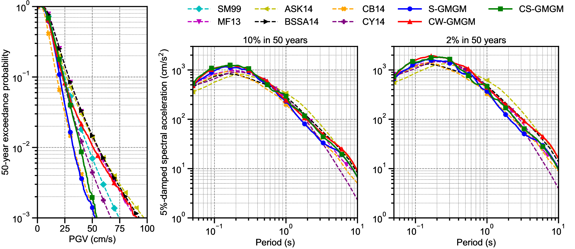
To verify the validity of the distribution of the sampled waveforms, we computed the PGV hazard curve and the 5%-damped uniform hazard spectra corresponding to 10% and 2% exceedance probabilities in 50 years, following the procedure described in the Calculation of IM exceedance probability subsection. These results were compared with those obtained from the conventional PSHA using GMMs, as shown in Figure 10. The analysis results are generally consistent, and the hazard analysis results obtained using the GMGMs fall within the inter-model variability of the GMM-based evaluations. Thus, the distribution of waveforms obtained using the proposed method can be considered appropriate. Next, we examine whether the number of samples is sufficient to evaluate the seismic hazard in a Monte Carlo sense. For the hazard analysis results of the S-GMGM, the evolution of the COV for each PGV level is shown in Figure 11. With c sim = 20, 000, the COV at the PGV level of 40 cm/s decreases to approximately 10%. A PGV of 40 cm/s corresponds to a 50-year exceedance probability of 0.0036 (i.e., a return period of approximately 13,900 years), indicating that the seismic hazard can be evaluated with reasonable accuracy up to a level sufficient for engineering applications. On the other hand, when hazard levels at lower exceedance probabilities are to be evaluated, or when a target COV of approximately 1% is required for the MCS, the current sample size of about 500,000 waveforms is insufficient. In particular, high-accuracy estimation in the low-exceedance probability range requires a substantially larger-scale analysis, and improving computational efficiency remains an important issue for future work. This aspect is discussed in more detail in Conclusion and discussion section.

The CW-GMGM and CS-GMGM can directly generate waveforms by specifying the required conditional labels, whereas the S-GMGM must repeatedly generate samples until waveforms corresponding to the required conditional labels are obtained. Since the distributions of conditional labels generated by the S-GMGM generally match those of the observed records, the occurrence frequency of waveforms with large magnitudes and short distances becomes extremely low. Consequently, a large number of generations is required before obtaining waveforms that satisfy the target conditions, resulting in a significant increase in computational cost. This advantage in computational efficiency is one of the key characteristics of the cGAN-based GMGMs.

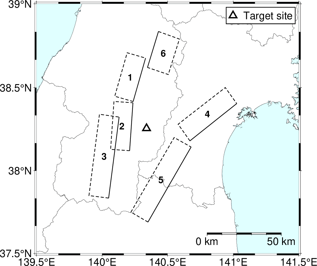
Figure 12 shows the spatial distribution of the target site and the source faults considered in this numerical example. The target site is located in the Tohoku region of Japan. The V S30 value at the site is 356 m/s and was obtained from the Japan Seismic Hazard Information Station (J-SHIS) database. Six source faults located near the site were selected from the active fault evaluations by the Headquarters for Earthquake Research Promotion (HERP) (The Headquarters for Earthquake Research Promotion, 2025). The earthquake occurrence models of the selected faults are shown in Table 2. When information on past earthquake occurrences is available for a given source fault, the BPT distribution is used as the occurrence model; otherwise, a stationary Poisson process is used. In this study, the earthquake occurrence models, their parameters, and the values of M W were determined based on the evaluations published by HERP. Source faults 1, 3, 5, and 6 follow the BPT distribution, while the others follow the stationary Poisson process. The values of R RUP were computed based on the locations of the specified source faults. In the earthquake occurrence model based on the BPT distribution, the probability P (E; T cur , ∆t) that an earthquake E will occur within the next ∆t years is computed as:

in which T cur is the number of years elapsed since the most recent earthquake, and µ and α are the parameters of the BPT distribution. 2.

Table 2: List of earthquake occurrence models for the source faults shown in Figure 12. µ and α are the parameters related to the mean and variability of the BPT distribution, respectively; ν is the annual earthquake occurrence rate for the model following a Poisson process; and T cur is the number of years that have elapsed since the most recent earthquake on the source fault.

No We assumed that the probability of multiple earthquake occurrences within the 50 years is negligible when the BPT distribution is used, and earthquake occurrence simulations were conducted by setting ∆t = 50. No restriction is imposed on the number of earthquakes that may occur within 50-year period in the occurrence model based on the stationary Poisson process. Earthquake occurrences were assumed to be independent across the source faults. We set delta functions as the probability distributions of r and m, and the values of M W and R RUP listed in Table 2 were used as fixed parameters. Based on these settings, ground-motion waveforms were sampled using Algorithm 1 with a target number of samples N w = 20, 000. As a result, 20,000 waveforms were obtained for the S-GMGM, CW-GMGM, and CS-GMGM, respectively. The corresponding values of c sim were 230,449, 226,172, and 228,059, respectively. For the S-GMGM, the same tolerances as those used in numerical example 1 were applied. The sampled ground motions were post-processed following the same procedure described in the Training results subsection. The computational environment was identical to that used in numerical example 1.

Figure 13 shows the hazard analysis results obtained using the S-GMGM. The results obtained with the CW-GMGM and CS-GMGM are shown in Figures S33 andS34, respectively. The earthquake occurrence probabilities in the MCS for each source fault are generally consistent with the probabilities computed from the parameters listed in Table 2. Note that source faults 3 and 5 did not generate any events throughout the MCS because their occurrence probabilities are extremely low. The sampled waveforms show relatively large amplitudes in the near-fault setting and for larger M W , indicating that reasonable waveforms were sampled for each source fault.

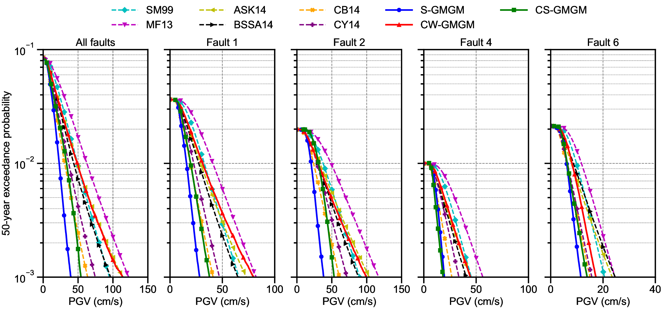
To examine the validity of the distribution of the sampled waveforms, we computed PGV values from the sampled ground motions and evaluated the 50-year exceedance probability of PGV using the method described in Calculation of IM exceedance probability subsection. In addition, to examine the influence of each source fault, we sampled 20,000 waveforms for each source fault using Algorithm 1 and computed PGV hazard curves in the same manner. These results were compared with those obtained using the GMMs, as shown in Figure 14. The hazard curves derived from

)DXOWPRGHO the GMGMs and GMMs exhibit generally good agreement, indicating that the distribution of the sampled waveforms is also reasonable. On the other hand, when examining the GMGM results individually, it can be seen that the S-GMGM and CS-GMGM tend to exhibit lower PGV evaluations than the GMMs, whereas the CW-GMGM tends to produce relatively larger PGV values. To consider the cause of this discrepancy, we first compare the results of the GMGMs with the SM99 and MF13 GMMs, both developed for Japan. Because the GMGMs treat the two horizontal components independently while the GMMs use the maximum amplitude of the two horizontal components or RotD100 as the IM, the PGV values from the GMGMs should, qualitatively, be smaller. Consistent with this expectation, the S-GMGM and CS-GMGM always produce lower estimates than the SM99 and MF13 GMMs. However, the CW-GMGM yields PGV values larger than those of the SM99 GMM in some cases. For the NGA-West2 GMMs, because RotD50 is used for the IMs, the PGV level should qualitatively be comparable to that of the GMGMs. However, the S-GMGM and CS-GMGM still yield lower estimates.

These differences may arise from the distinct DNN architectures used in the GMGMs and from differences in how variability is modeled between the GMGMs and the GMMs. Faults 1, 2, and 4 correspond to conditions involving M W 6.8 or 6.9 and relatively short distances, where the number of observed records is limited and model training becomes challenging. Although the S-GMGM and CS-GMGM share relatively similar DNN architectures, they differ from that of CW-GMGM; thus, the learning behavior in such data-sparse regions may vary depending on the model architecture.

Regarding the variability in these data-scarce regions, GMMs model variability using a lognormal distribution, allowing the variability to be specified based on seismological and earthquake engineering knowledge even when data are limited. In contrast, GMGMs learn to approximate the empirical distribution of the training dataset itself. Therefore, in magnitude-distance bins with very few observed records, the variability of the ground-motion waveforms may be underestimated due to the scarcity of data.

Based on the above considerations, hazard analysis results obtained using GMGMs may exhibit variability arising from factors different from those in GMM-based evaluations. Therefore, in hazard analysis using GMGMs, it is desirable to develop multiple GMGMs using different approaches or by different researchers, and to integrate the results using a logic-tree framework similar to that employed in conventional PSHA.

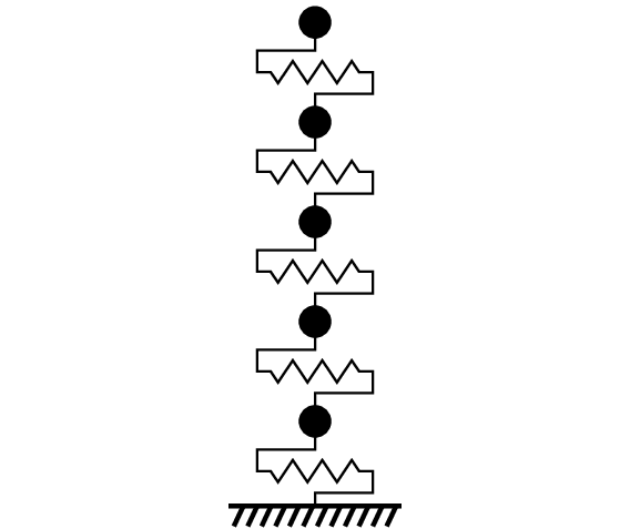
Assuming that a building exists at the target site considered in numerical example 2, nonlinear dynamic response analyses were conducted using the sampled ground motions as input. The building model is shown in Figure 15, and the model parameters are summarized in Table 3. A 5DOF system was considered, and a bilinear hysteresis model was adopted. The yield displacement was defined as the displacement corresponding to an inter-story drift angle of 1/100, and the stiffness degradation ratio was set to 0.05. proportional damping was used. The first and second natural periods of the building model are approximately 0.91 s and 0.31 s, respectively. As the EDP, the maximum inter-story drift of each story is used.

Using the 20,000 ground motions sampled by the S-GMGM, G wav = {g i,j,k }, the relative displacement response waveforms for each story, d, were computed to obtain the set R = {d i,j,k,l | l = 1, • • • , 5}. Here, the subscript l denotes the story index. Since the sampled ground-motion waveforms follow the seismic hazard, the set R also represents the probability distribution of building responses that reflect the seismic hazard. Therefore, the exceedance probability of the maximum inter-story drift, EDP i,j,k,l , computed from each waveform in R, can be evaluated using the same procedure described in Calculation of IM exceedance probability subsection as: Figure 16: 50-year exceedance probability of the maximum interstory drift for each story, based on the ground motions evaluated as the seismic hazard for numerical example 2 using the S-GMGM.

in which P l (EDP > a; t) is the t-year exceedance probability of the EDP for story l. Figure 16 presents the 50-year exceedance probabilities of the maximum inter-story drift for each story. These results demonstrate that the evaluation of EDPs directly from the seismic hazard is straightforward using the proposed method.

In the proposed waveform-based PSHA, each waveform in G wav retains the corresponding information from the earthquake catalog of MCS. Therefore, each building response waveform d i,j,k,l and each EDP i,j,k,l is associated one-to-one with magnitude and distance information. This enables hazard disaggregation targeting EDPs. For a case in which an EDP exceeds a specific level a in t-year time period, the disaggregation of PSHA can be formulated as:

in which B M,R is the set of source indices i whose magnitude M and distance R values fall within the bin corresponding to (M, R). Figure 17 shows the disaggregation results for cases in which the maximum inter-story drift exceeds 0.5 cm in 50 years. It can be seen that the hazard contributions are different between the first and third story. For example, the histogram bins near M W = 6.6 in Figure 17 corresponds to the contribution from the response analyses excited by ground motions associated with Fault 6. Note that the variation in the magnitude-distance values arises from the acceptance tolerance in the sampling procedure of the S-GMGM. It can be seen that Fault 6 may cause larger damage on the first story compared with the third story. Thus, the proposed method, which conducts PSHA based on ground-motion waveforms, allows the seismic hazard results to be analyzed not only in terms of IMs but also in terms of building response. It should be noted, however, that the GMGM used in this study considers only M W as the source characteristic. Therefore, the results presented in Figure 17 do not reflect fault-specific characteristics beyond magnitude. Future development of GMGMs incorporating more detailed source characteristics is expected to enable seismic design and risk assessment that more closely integrate SSC considerations with building seismic response.

We proposed a novel framework for PSHA, named waveform-based PSHA, that can directly evaluate the distribution of ground-motion waveforms. We presented the mathematical formulation of the waveform-based PSHA as well as an MCS algorithm for its implementation. As a method for modeling the probability distribution of ground-motion waveforms, we adopted GAN-based deep generative models and developed three GMGMs. We proposed a method for quantitatively evaluating the performance of GMGMs and confirmed that the trained GMGMs are capable of generating high-quality ground-motion waveforms and accurately capturing their probability distributions. Subsequently, hazard analyses using the proposed method were performed for two numerical examples: one involving a hypothetical area source and another involving an actual site and source faults in Japan. We demonstrated that seismic hazard can be represented as a set of ground-motion waveforms and validated the analysis results by comparing the IM-based hazard derived from these waveforms with the results of conventional PSHA using GMMs. Finally, nonlinear dynamic response analyses of a building model were conducted using the ground motions from the evaluated seismic hazard, and it was demonstrated that the exceedance probabilities of EDPs, as well as hazard disaggregation with respect to EDPs, can be analyzed in a straightforward manner.

Although the proposed hazard evaluation requires MCS using deep learning models, the GAN-based generative models employed in this study have low computational cost for data generation, and the MCS computation is relatively inexpensive for the cGAN-based models. On the other hand, for the GMGM that model joint distribution of groundmotion waveform and its conditional label, analyses become inefficient in regions where observed records are sparse. In this study, MCS was performed so that the COV was approximately 10%, but achieving a COV on the order of 1% would require substantially more iterations of MCS. Improving the computational efficiency of the proposed method by using importance sampling (e.g., Houng and Ceferino (2025)) is an important direction for future work.

The three GMGMs used in this study were trained based on the same dataset, however, relatively large differences were observed in the resulting hazard curves. As a possible factor of such differences, we identified in Example 2: actual site and source faults subsection the influence of variations in the DNN architectures used in the GMGMs. Another potential factor is the effect of the training state of the GMGMs. When hazard analyses were conducted using GMGMs at different training epochs, the resulting hazard curves differed significantly in some cases. Since the optimization algorithms used in deep learning do not guarantee convergence to a global optimum, a model trained using the same dataset and DNN architecture does not necessarily produce identical hazard estimates. In other words, while extending GMMs to deep learning-based models has enabled the evaluation of ground-motion distributions at the waveform level rather than at the IM level, it has also increased the sources of epistemic uncertainty. Accordingly, further advancement of quantitative performance evaluation methods for GMGMs, such as the approach proposed in Optimal Epoch Selection Method subsection, is particularly important.

In this study, only three explanatory variables, M W , R RUP , and V S30 , were used to characterize ground-motion waveforms. While incorporating additional explanatory variables is an important direction for future development, such modeling requires a larger number of observed records for training. Thus, the compilation of a large-scale waveform database is another essential task for future research. Moreover, because this paper focuses solely on ground-motion modeling, further advancement of SSC and GMC within the proposed framework also constitutes an important topic for future investigation. Xu, Z. and J. Chen (2024). High-resolution ground motion generation with time-frequency representation. Bull. Earthq. Eng. 22, 3703-3726. Yamaguchi, J., Y. Tomozawa, and T. Saka (2024). Site-specific ground-motion waveform generation using a conditional generative adversarial network and generalized inversion technique. Bull. Seismol. Soc. Am. 114(4), 2118-2137.

A Appendix A

A.1 Definition of the indices of ground-motion characteristics used in this study We used the JMA instrumental seismic intensity proposed by the Japan Meteorological Agency (JMA) as a measure of seismic intensity. While the original JMA instrumental seismic intensity is defined using all three components of ground motion, it was calculated using only a single horizontal component in this study. First, a bandpass filter F (f ) defined by the following equations is applied to the acceleration time-history data:

where F l , F h , and F t represent the low-cut filter, high-cut filter, and the filter for the effect of period, respectively. f 0 and f c are constants and we set to 0.5 and 10, respectively. ξ 4 is then calculated as: ξ 4 = 2 log 10 a + 0.94 (29) in which a is the threshold level for which the total duration of ground-motion data exceeding |a| is 0.3 s. Following the JMA definition, the computed value of ξ 4 was rounded to the third decimal place and then truncated at the second decimal place.

The predominant frequency ξ 5 was calculated from the Fourier amplitude spectrum smoothed using a Parzen window with a bandwidth of 0.5 Hz.

The zero-level crossing rate, ξ 6 , was computed as the average of the zero-level up-crossing and down-crossing rates. Since the ground-motion waveforms used in this study were clipped to fixed time windows (81.92 s or 40 s) to serve as inputs for the deep-learning models, the calculation of ξ 6 was limited to the portion corresponding to the time interval of D 5-95 in order to reduce the effects of waveform truncation.

The negative maxima and positive minima, originally introduced by Rezaeian and Der Kiureghian (2010) as indices corresponding to the bandwidth of ground motions, indicates that ground motion with wider bandwidth tends to have a larger number of negative maxima and positive minima. In this study, the average number of negative maxima and positive minima per unit time was used as ξ 7 . Similar to the calculation of ξ 6 , the computation was limited to the vibrations within the time interval corresponding to D 5-95 .

Significant duration, D 5-95 , is known as a measure of the duration of ground motion and is calculated as follows: in which a(t) is the acceleration at time t, t r is the total duration of the records, and t 5 and t 95 is the time that the cumulative power of the ground motion to reach 5% and 95% of the total cumulative power, respectively. The value of D 5-45 is known to correspond to the time at the middle of the strong-shaking phase (Rezaeian and Der Kiureghian, 2010), and is calculated as follows: where t 45 is the time that the cumulative power of the ground motion to reach the 45% of the total cumulative power.

Arias intensity is a measure of total energy contained in the ground motion. Although it is generally defined over the entire duration of the waveform, it was calculated only for the portion corresponding to D 5-95 as follows for the same reason described in the calculation of ξ 6 :

in which g is the gravitational acceleration and we set g = 980.665 cm/s 2 . There are several definitions of spectrum intensity. In this study, we adopted that proposed by Housner (1961):

in which S V (T, ζ) is the spectral velocity, T is the natural period, and ζ is the damping ration, which was set to 5%. The mean period, representing the overall frequency characteristics of the waveform, was computed following the definition of Rathje et al. (1998):

in which f i is the discretized frequency and C i is the Fourier amplitude at f i .

B.1 GMM formulations used in this paper

The SM99 GMM targets only PGA and PGV, and for crustal earthquake, PGV is evaluated by the following equation:

in which D is the hypocenter depth (unit: km). In the Training results subsection, considering that the GMGMs are developed with the observed records of crustal earthquakes, we set D = 10 km. The SM99 GMM evaluates the IMs on the hard rock site condition with an average shear-wave velocity of 600 km/s. To account for the amplification of the surface soil, the PGV values were corrected using the empirical relationship of Fujimoto and Midorikawa (2003):

For the variability, the following equation, which was used in Fujiwara et al. (2023), was employed:

in which σ is the base-10 logarithmic standard deviation of PGV.

Among the model proposed in Morikawa and Fujiwara (2013), a model with a quadratic magnitude term was adopted.

The median value of IMs was evaluated using the following equations:

in which a, b, c, d, e, M W0 , M W1 , p s , V 0 , and V S max are coefficients. G s is the correction term for amplification by shallow soft soils. The variability of PGV and Sa was evaluated in equation ( 37) as in the practice of Fujiwara et al. (2023).