DeXposure: A Dataset and Benchmarks for Inter-protocol Credit Exposure in Decentralized Financial Networks

However, these findings are often theoretical and scenario-based (European Systemic Risk Board, 2023), or limited to specific measurement issues without providing a systemwide quantitative map of inter-protocol credit exposures (Luo et al., 2024). This highlights a critical need for a large-scale, real-world dataset modelling TVL information with network modeling to enable macro-level, quantitative analysis for the DeFi ecosystem.

This paper aims to address this gap by constructing DeXposure, the first large-scale dataset for inter-protocol credit exposure in decentralized financial networks, encompassing thousands of protocols that represent the majority of DeFi. Here, A DeFi protocol is a set of programs implemented through smart contracts (Auer et al., 2024) on a blockchain. These programs generate digital claims that represent credit derived from underlying assets, which ultimately originates from the native tokens of the respective blockchains (Auer et al., 2025).

The collected DeXposure dataset comprises 43.7 million entries covering 4.3 thousand protocols, 602 blockchains, and 24.3 thousand unique tokens, spanning 2020 to 2025, providing unprecedented scale and temporal coverage for analysis in the field. We introduce a new concept value-linked credit exposure that refers to the inferred financial dependency relationships between protocols derived from changes in their TVL patterns. Credit exposure emerges when tokens generated by one protocol (the issuing protocol) are held or locked within other protocols. By constructing this inter-protocol credit exposure network, we aim to reveal broader patterns and dynamics of exposure relationships within the DeFi ecosystem that were previously difficult to discern. This approach overcomes the limitations of existing studies that often focus on a small number of protocols or rely solely on transactional metrics (Kitzler et al., 2022;Badev and Watsky, 2023). It allows a more comprehensive view of exposure changes within the ecosystem, tracking how financial dependencies between protocols evolve.

We develop three benchmarks for machine learning tasks with financial applications: (1) graph clustering for measuring the global credit exposure network (Chan-Lau, 2018), (2) vector autoregression for analyzing network dynamics during major market shocks (such as the collapses of Terra (Lee et al., 2023) and FTX (Conlon et al., 2024)), and (3) temporal graph neural networks (Rossi et al., 2020) for predicting dynamic links (Dileo et al., 2024). Our findings can provide implications for policymakers, central bankers, and regulators by revealing exposure dynamics, market structure evolution, and systemic risk factors. These results can also enhance the capacity to monitor and predict the dynamics of the DeFi market.

To support reproducibility, we publicly release our dataset and code at https://github. com/dthinkr/DeXposure. We also present our results through an interactive DeFi digital tool https://ccaf.io/defi/ecosystem-map/visualisation/graph .

This section provides an overview of DeFi protocols, the TVL metric, and recent research in the field, setting the context for our study.

Unlike traditional finance, where the International Organization for Standardization (ISO) provides a comprehensive framework for classifying financial instruments (International Standard Organization, 2021), no such standardized taxonomy exists for DeFi. This lack of standardization complicates analysis. Zetzsche et al. (2020) broadly classify DeFi applications into four categories: (1) deposit taking and lending, (2) trading and investments, (3) insurance, and (4) auxiliary services. Examples include lending protocols such as Aave and Compound, decentralized exchanges such as Uniswap, and yield aggregators such as Yearn Finance (Schär, 2021;Auer et al., 2024). Werner et al. (2022) provide a more granular classification, identifying seven main categories of DeFi protocols: (1) decentralized exchanges, (2) lending platforms, (3) derivatives, (4) asset management, (5) insurance, (6) payment channels, and (7) stablecoins. Their systematization maps these categories to prominent protocols such as Uniswap (DEX), Compound (lending), Synthetix (derivatives), and DAI (stablecoin) (Schär, 2021;Auer et al., 2024). Xu et al. (2021) provide a systematic analysis of Decentralized Exchanges (DEXs) with Automated Market Maker (AMM) protocols, highlight the transition from traditional banking to DeFi lending (Xu and Vadgama, 2022), and provide a comprehensive survey of business models across different types of DeFi protocols (Xu and Xu, 2023). However, protocol-based classifications often fall short for multi-utility protocols, where one protocol is associated with multiple categories. Understanding each protocol’s underlying assets and liabilities would pave the way for instrument-based classification, which aligns with established taxonomies (International Standard Organization, 2021), though this remains challenging due to data heterogeneity.

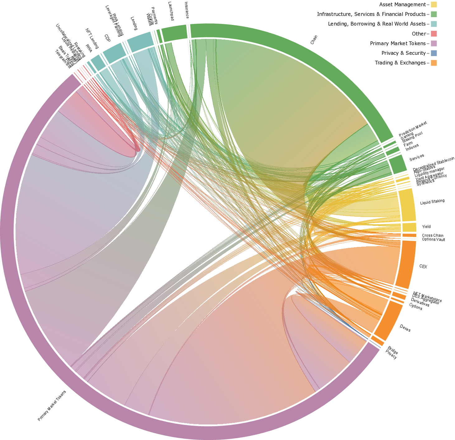
DefiLlama, a DeFi analytics platform, currently categorizes protocols into dozens of categories (DefiLlama, 2024). While this granularity is useful for detailed analysis, it can complicate broader ecosystem-level insights. In this work, we map these numerous De-fiLlama categories into a set of broader, more concisely defined groups, which enhances clarity. Table 1 presents our categorization scheme.

In traditional finance, credit exposure represents the potential loss a lender faces if a borrower defaults (Basel Committee on Banking Supervision, 2023). In DeFi, credit exposure arises from token-mediated dependencies: when one protocol holds tokens issued by an- other, it becomes exposed to that protocol’s credit risk. Unlike traditional finance, where exposure is bilateral and explicitly contracted, DeFi exposure relationships form organically through protocol composability and user actions.

The token-based nature of DeFi creates complex networks of interdependency. A protocol that issues tokens establishes potential exposure pathways whenever those tokens are adopted as collateral, liquidity, or reserves by other protocols. These exposure relationships can propagate contagion during market stress, as the failure of one protocol can affect all protocols that hold its tokens. Recent empirical studies have examined credit exposure at the protocol level through liquidation mechanisms (Qin et al., 2021) and lending risk analysis (Doerr et al., 2025), providing evidence of the materiality of these exposure relationships.

Existing research has primarily focused on static network snapshots or small-scale analyses of individual lending protocols, based on transaction-level data. As DeFi grows in scale and interconnection with traditional finance, there is a critical need to track credit exposure dynamics across the entire DeFi ecosystem over extended time periods for regulatory monitoring, systemic risk oversight, and policy formulation. Understanding how exposure concentrations shift during market events, how new exposure pathways emerge, and how the network’s topology evolves provides essential insights for financial stability assessment, early warning systems, and the development of appropriate regulatory frameworks.

Total Value Locked (TVL) is a fundamental metric in decentralized finance that measures the total USD value of digital assets deposited and held within a DeFi protocol at any given time (DefiPulse, 2021). Developed by DeFi Pulse (DefiPulse, 2021) and popularized by DefiLlama (DefiLlama, 2021a), TVL serves as a key indicator of a protocol’s size, popularity, and market significance. For example, if users have deposited $100 million worth of various cryptocurrencies (such as Bitcoin (Nakamoto, 2008), Ethereum (Buterin, 2014), or fiatreferenced stablecoins (Lyons and Viswanath-Natraj, 2020)) into a lending protocol, that protocol's TVL would be $100 million. As users deposit or withdraw assets, the TVL fluctuates accordingly, providing insights into capital flows and protocol adoption. The metric quantifies the token assets held within a DeFi protocol and computes their currency value based on associated token prices. The calculation of TVL faces challenges due to the heterogeneous nature of DeFi protocols, which lack a unified accounting standard.

Additionally, DeFi protocols function primarily as credit instruments, leading to issues of double counting or rehypothecation, similar to the money multiplier in banking (McLeay et al., 2014). While recent studies (Luo et al., 2024) have proposed methodologies to mitigate double counting, our perspective is that without a clear outline of credit and liquidity risks, the concept of double counting remains ambiguous, as credit inherently involves multiple claims on the same underlying assets. Thus, identifying and excluding double counting based on a token’s stage in circulation might overlook important market dynamics, specifically leverage and interconnectedness. Furthermore, confusion over a protocol’s assets and liabilities complicates TVL calculations, as some protocols compute TVL using liability tokens rather than asset tokens (DefiLlama, 2024), making it challenging to assess protocol solvency.

Despite these challenges, TVL remains a comprehensive metric that captures the scope of the DeFi landscape through its crowdsourced data from various protocol development teams. As of 2025, data providers such as DefiLlama track TVL for over 2,000 DeFi protocols across hundreds of blockchains (DefiLlama, 2024;Stepanova and Eriņš, 2021), providing a rich resource for analyzing the asset side of DeFi balance sheets.

Research on TVL, DeFi network analysis has attracted increased attention in recent years. Luo et al. (2024) introduced Total Value Redeemable (TVR) to address double counting in TVL calculations. Their analysis of 100 DeFi protocols showed TVR to be more stable than TVL during market downturns and quantified double counting through a DeFi money multiplier. Metelski and Sobieraj (2022) used correlation analysis and panel data models to examine relationships between TVL and other economic indicators, finding that protocol valuations depend on various performance measures, with TVL’s impact varying across metrics. Stepanova and Eriņš (2021) tracked TVL for 12 major DeFi applications over a 34-month period, documenting the rapid growth and concentration of activity in a small set of protocols.

Network analysis has provided key insights into DeFi’s complex interactions. Kitzler et al. (2022) studied compositions of 23 major DeFi protocols on Ethereum and constructed a smart-contract interaction network, showing that decentralized exchanges and lending protocols occupy central positions and that interactions concentrate in a strongly connected component, making DeFi structurally prone to contagion. Li et al. (2024) employed network analysis to research systemic risk in 30 DeFi protocols, finding that protocol interconnectedness can lead to contagion effects during market stress. Alamsyah and Muhammad (2024) analyzed 5.8 million transactions of three DeFi tokens on Ethereum. Using network metrics, they quantified market size, transactions per wallet, market density, and transaction clusters. Their centrality calculations identified key wallet addresses and their market roles.

Several studies have focused on specific aspects of DeFi. Znaidi et al. ( 2023) analyzed the Curve ecosystem over a 2-year period, highlighting its central role in DeFi. Weingärtner et al. (2023) examined cross-chain bridges in DeFi, emphasizing their growing importance and associated risks. Zhang et al. (2023) studied the evolution of automated market makers (AMMs) in DeFi over a 3-year period, tracking changes in protocol designs and market structures.

The advancement of DeFi has necessitated new empirical resources, leading to a recent surge in open-access datasets. These contributions primarily target three domains: security, market microstructure, and governance.

In the security domain, researchers have released extensive datasets to combat fraud. Sun et al. (2025) and Alhaidari et al. (2025) provide granular data on rug pulls across Ethereum, BSC, and Solana, facilitating the training of detection models. Suzuki et al. (2025) bridge on-chain and off-chain data to investigate token scams, while Carpentier-Desjardins et al. ( 2025) map the broader landscape of crypto-crime incidents.

For market microstructure and economic analysis, Chemaya et al. (2025) introduced daily transaction indices for Uniswap v3, enabling cross-chain comparisons of DEX liquidity. Chen and Tsai (2025) established benchmarks for yield prediction on Curve Finance. In governance, Ma et al. (2025) compiled a comprehensive corpus of smart contract audit reports to analyze voting vulnerabilities.

Despite these advancements, existing datasets are largely segmented by specific verticals (e.g., fraud, specific DEXs) or event types. There remains a scarcity of longitudinal, ecosystem-wide data that captures the interconnected balance sheets of protocols.

This section outlines our approach to building a large-scale DeFi network dataset designed for machine learning applications. We transform unstructured on-chain value states into a structured temporal graph {G τ } suitable for tasks such as dynamic link prediction, graph clustering, and anomaly detection. Our methodology addresses the challenge of converting raw TVL data into a coherent network topology that preserves the temporal dependencies required for learning dynamic market behaviors.

We begin by formally defining the foundational concepts and data structures underlying our network construction.

We define the data model formally. Let P be the set of all protocols, C the set of all chains, and X the set of all tokens. Each token § ∈ X at any given time t is characterized by a tuple (n t , v t ), where n t represents the amount of the token, and v t represents the USD value of the token.

The relationship between protocols, chains, and tokens is modeled using a mapping: R : P × C → 2 X , where 2 X denotes the power set of X , representing all possible subsets of tokens with their associated attributes. This mapping allows each protocol-chain pair to be associated with a dynamic subset of tokens. For instance, consider a protocol p ∈ P operating on a blockchain c ∈ C. The mapping R(p, c) might yield a subset of tokens { § 1 , § 2 , . . . , § k } ⊂ X , where each token § i at time t is represented as:

(1

To analyze the global state of a token across all protocols and chains, we define the global state of token § i at time t as Θ § i (t). This global state is an aggregation of the token’s amounts and values from all protocol-chain pairs where the token is present and is represented by:

where R -1 ( § i ) denotes the set of all protocol-chain pairs (p, c) that include token § i , n

represents the amount of § i under protocol p and chain c at time t, and v

represents the USD value of § i under the same conditions.

We define two additional types of global states: protocol-wise token state and chain-wise token state:

For a given protocol p or a chain c at time t, equations 3 and 4 describe the aggregated state of token § i for both amount and value. They enable the global analysis of token behavior within specific protocols or chains. For example, we can answer questions such as: how much token i is locked within a DeFi protocol, or a blockchain at a historical time point. Such answers are derived from this data model and are documented in our published tool (Cambridge Center for Alternative Finance, 2024).

Definition 1 (Credit Exposure) Let X G (q) denote the set of tokens that protocol q generates or issues, and let X p (t) denote the set of tokens currently held (locked) by protocol p at time t. Protocol p has credit exposure to protocol q if:

(5)

This means tokens generated by q are currently locked in p, creating a financial dependency. If tokens issued by q lose value or become illiquid, protocol p faces exposure to this risk.

To illustrate this concept, Figure 1 shows how credit exposure emerges in DeFi. A user wraps ETH to WETH through the WETH protocol, then uses WETH as collateral in Mak-erDAO to generate DAI. This creates credit exposure from MakerDAO to the WETH protocol-if WETH fails, MakerDAO’s collateral is at risk. The figure shows the balance sheet positions: WETH protocol holds ETH as assets with WETH as liabilities, while MakerDAO holds WETH as assets with DAI as liabilities, creating a chain of credit dependencies. Our approach measures the dynamics of these credit exposure relationships over time through changes in TVL. As token holdings shift between protocols, exposure relationships strengthen, weaken, or dissolve.

We retrieve our data from DefiLlama (DefiLlama, 2021a). Figure 2 offers a visual assessment of data distribution over time. The heatmap illustrates data availability and granularity for all recorded DeFi protocols, identified by numeric IDs. Each dot indicates at least one data entry per date. Color density varies with data granularity: darker shades denote higher frequencies, such as hourly updates, while lighter shades suggest less frequent updates, like daily ones.

We detail the construction and analysis of our network dataset, which is designed to capture the dynamic inter-protocol credit exposure relationships between different DeFi protocols over discrete time intervals through changes in Total Value Locked.

Let t represent discrete time steps over which the network is analyzed, with T being the set of all such steps. First, define X p to represent the set of tokens associated with a protocol p at a given time t. This can be expressed from the mapping R which relates protocols and chains to tokens:

Define stock S t as the USD value at time t of an entity, where the entity can be either a protocol p or a chain c. For example, the total stock of a protocol p at a given time t is calculated by aggregating the USD value v t of all tokens § within the protocol:

Define time interval τ := t 2 -t 1 , where t 1 and t 2 are consecutive time points in T . The change in stock for a protocol p over the interval τ is calculated by aggregating the changes in stock values of all tokens § within the protocol over that interval. This can be represented as:

∆S p,τ := §∈Xp(t)

where ∆v § p,τ := v § p,t 2 -v § p,t 1 is the change in stock of token § at protocol p over the interval τ , and the change of token state can be described by ∆ § p,τ = (∆n § p,τ , ∆v § p,τ ).

Given a token § in protocol p, the mapping function M determines the issuing protocol q that generates token §. The issuing protocol is the protocol that generates or manages a given token, establishing the foundation for credit exposure relationships. Using this function, we are able to map a token in protocol p to its issuing protocol q. This mapping ensures that changes in token holdings in protocol p can be attributed to exposure relationships with the issuing protocol q, q = M( § p,τ ). ( 9)

To ensure accurate and comprehensive mapping M, we design four methods that are applied in a fall-back manner:

1. Tokens are directly mapped to protocols based on the metadata list sourced from DefiLlama (DefiLlama, 2021b), where token names are listed along with specific protocols. This method is straightforward and relies on source data where the relationship between tokens and protocols is already identified.

2. In cases where direct lookup is not possible, tokens are manually mapped to protocols. This involves human intervention to categorize tokens based on expert knowledge and available documentation. We create a manual mapping for tokens with the highest average historical TVL. Table 2 shows a selection of the top tokens defined in this way.

3. For tokens that are not covered by the first two methods, we employ a more sophisticated approach involving textual analysis:

(a) Textual Representation: Each token § and protocol p is represented by a set of descriptive texts extracted from metadata fields, which we denote as Texts § and Texts p .

(b) Vectorization: Textual data is transformed into numerical vectors using the Term Frequency-Inverse Document Frequency (TF-IDF) (Qaiser and Ali, 2018;Ramos, 2003) method. We can therefore derive vector representations V § and V p for each token and protocol,

(c) Cosine Similarity Calculation: We calculate the similarity between the vectorized representations of tokens and protocols using the cosine similarity metric. The similarity score S( §, p) is given by:

(d) Thresholding and Mapping: Tokens are mapped to the protocol with the highest similarity score, provided that the score exceeds a predefined threshold θ. Where M( §) denotes the mapping of token § to a protocol, this mapping is formally defined as:

4. If a token cannot be mapped to an existing protocol p through any of the above methods, i.e., it does not pass through the TFIDF threshold, it is categorized under a protocol with its own token name. This serves as a catch-all for tokens that do not fit into any other mapping criteria. We categorize these protocols as Primary Market Tokens. Tokens that fall into this category are, for example, WETH, which are protocols that handle or produce a single token.

We describe the interactions between DeFi protocols over discrete time intervals τ using a series of weighted directed graphs, where each graph corresponds to a snapshot of interactions within a network of DeFi protocols at discrete time intervals. Here, we focus on modeling each snapshot instead of exploring its temporal relationship. Consider each graph snapshot as G τ = (P τ , E τ ). We define the weighted set of vertices as:

where P is the set of all possible DeFi protocols under consideration, and w (p) represents the assigned weight to protocol p.

The weighted edge set is defined as:

where E represents all possible directed interactions within the network, and w (e pq ) quantifies the interaction strength from p to q. Given a time interval τ := t 2 -t 1 , the vertice weight is defined by:

This equation sums the USD values v §,t 2 of each token § within protocol p at time t 2 , where § is decided by the tokens that are present in the protocol at both the beginning and the end of the interval τ .

To introduce edge weight, we define the value flow of a single token from p to q as:

This means the total value flow between any two protocols will remain positive. If negative, we reverse the flow direction. Based on this, we can define edge weight simply as:

Where q = M ( § p,τ ). This means that weight is calculated by considering all the token flows between p and q, as indicated by M. Conceptually, the edge weight w τ (e pq ) represents the change in credit exposure from protocol p to the issuing protocol q over the time interval τ . A positive edge weight indicates increasing exposure (tokens flowing from p to q), while the magnitude quantifies the extent of the exposure change.

For single-token protocols, where each protocol is associated via M with only one specific token §, the edge weights are directly equivalent to the flow of that token. Therefore, for such protocols, the flow F § for any edge e is equal to the weight of the edge w(e). This can be expressed as:

The procedure to calculate edge weights is described in Algorithm 1.

Algorithm 1 Calculate Edge Weights for Single Network Snapshot Require: R: Mapping of protocols, chains, and tokens Ensure: Network G = (P, E) 1: procedure GenerateNetwork(R)

Initialize P ← ∅, E ← ∅

Let P be the set of all unique protocols and chains derived from R 4:

for each protocol p ∈ P do for each link (p, q) ∈ E do 19:

Compute edge weight: w(e pq ) ← §∈Xpq F § 20:

end for

Format P to include node attributes such as category 22:

return G = (P, E) 23: end procedure 24: procedure PrepareEdge(R)

Initialize E ← ∅ 26:

else 30:

end for 33:

return E 34: end procedure

In Table 3, the DeXposure dataset provides daily snapshots of DeFi credit exposure networks in a structured JSON format. Each entry is indexed by date (e.g., “2020-03-23”) and contains two core components: a nodes list and a links list. The nodes field describes DeFi protocols or tokens, each represented by an identifier (id), the protocol’s total asset value in USD (size), and a detailed breakdown of token-level holdings (composition). The links field captures directed credit exposure relationships between protocols, specifying the source, target, exposure size in USD, and a token-level composition indicating the contribution of each asset to the exposure.

This dataset contains both balance-sheet information (via nodes) and inter-protocol dependencies (via links), enabling the reconstruction of market dynamic, multi-token credit exposure networks, and the temporal analysis of changes in the network. As of October 2025, the dataset covers more than 4,300 protocols, 602 blockchain networks, and 24,300 unique tokens, with all numerical values denominated in USD. JSON files are provided alongside CSV formats to support scalable downstream analysis.

We characterize the DeXposure dataset and demonstrate its utility through three benchmarks: (1) global network measurement capturing the structural evolution of credit exposure networks, (2) sector-level credit exposure dynamics during major market shocks (Terra and FTX), and (3) dynamic link prediction on temporal graph neural networks. These benchmarks illustrate how our dataset enables macro-level tracking and analysis of credit exposure evolution in the DeFi ecosystem.

This benchmark characterizes the structural properties of the credit exposure network through edge composition analysis, network metrics, and visualization techniques.

Our objective is to characterize the structural evolution of the credit exposure network constructed in Section 3.3. Recall that our dataset consists of a temporal sequence of weighted directed graphs {G τ } τ ∈T , where each snapshot G τ = (P τ , E τ ) represents the credit exposure relationships between DeFi protocols at discrete time intervals. Each node p ∈ P τ represents a protocol with weight w(p) indicating its total value locked, and each directed edge e pq ∈ E τ captures credit exposure from protocol p to protocol q with weight w(e pq ) quantifying the exposure magnitude.

We aim to answer the following questions: (1) How does the network’s structural complexity evolve over time? (2) What are the patterns of connectivity and centralization as the DeFi ecosystem matures? (3) Can we identify distinct clusters or communities of protocols, and how do these clusters change? To address these questions, we employ three complementary approaches: edge composition analysis to understand the token diversity underlying exposure relationships, network-level metrics to quantify structural properties such as centralization and clustering, and dimensionality reduction combined with clustering algorithms to visualize and identify protocol groupings in the high-dimensional feature space.

We calculate several network metrics to characterize the global properties of our credit exposure network and track its evolution over time:

1. Degree Centralization:

where d max is the maximum total degree and d i is the total degree of protocol i.

For our directed graph, we define the total degree as the sum of the in-degree and out-degree for each node.

2. Degree Coefficient of Variation:

where σ d and µ d are the standard deviation and mean of the total degree distribution, respectively.

3. Degree Distribution Entropy:

where p(k) is the probability of a protocol having total degree k.

4. Top 10% Degree Concentration:

where total degrees are sorted in descending order.

5. Assortativity:

where e jk is the joint probability distribution of the total degrees of two protocols at either end of a randomly chosen edge, and q k is the distribution of the total degree.

where d(i, j) is the shortest path length between protocols i and j. For our directed graph, we consider the shortest directed path from i to j.

As edges between any two nodes are aggregated, there is no edge multiplicity within any snapshot. We define composition length of an edge in the network as the number of distinct tokens that are associated with that edge. Therefore, for an edge e connecting protocols p and q, the composition length is given by the cardinality of the set of tokens X pq associated with that edge, i.e., |X pq |. Figure 3 shows the 30 edges with the highest token composition length in the earliest snapshot of each year, excluding the value transfers that are sourced to Unknown.

Table 4 provides an overview of the credit exposure network dynamics over four years from 2020 to 2024, indicating substantial expansion. The degree centralization peaked in 2021 before decreasing, suggesting an initial concentration followed by a more decentralized structure. The degree coefficient of variation increased from 2020 to 2021, then stabilized, indicating persistent inequality in connections. The degree distribution entropy generally increased, suggesting growing complexity in connection patterns. The top 10% degree concentration remained high after 2021, indicating that a small fraction of nodes consistently held a large share of connections. Assortativity remained negative but improved slightly, indicating diverse, interdependent connections. The average closeness centrality increased, suggesting improved network efficiency for exposure propagation.

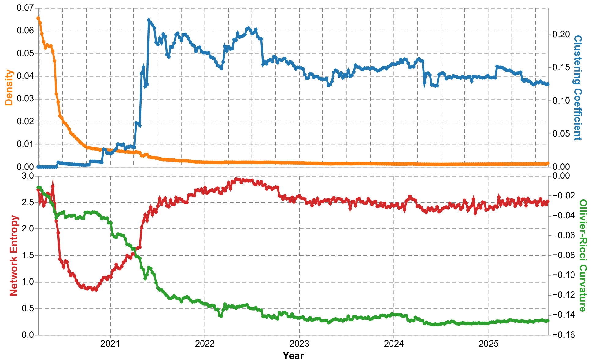
In Figure 4, we observe trends in network density, clustering coefficients, network entropy, and Ollivier-Ricci curvature over time. The density decreases and stabilizes at a lower level, indicating a reduction in connections relative to possible maximums as the network expands. The clustering coefficient remains high, suggesting the preservation of local clustering properties and subgroup cohesion, a result of our stock-and-flow mapping. Network entropy stays within a narrow range due to consistent structural complexity. Ollivier-Ricci curvature fluctuates in negative values, indicating fluctuations in global connectivity. These metrics show our network snapshots decrease in density but maintain local clustering and complexity.

To understand the structural dynamics of the credit exposure network over time, we employ dimensionality reduction and clustering techniques. This allows us to visualize highdimensional network data in a two-dimensional space and reveal protocol relationships and market structure that are not immediately apparent from raw network metrics.

Figure 5 illustrates the temporal evolution of the DeFi network structure from 2021 to 2024 using t-Distributed Stochastic Neighbor Embedding (t-SNE) (Maaten and Hinton, 2008) visualization combined with Density-Based Spatial Clustering of Applications with Noise (DBSCAN) (Ester et al., 1996). Each subplot represents a snapshot of the network for a specific year. The protocols are positioned in a two-dimensional space based on their network attributes, including degree centrality, betweenness centrality, eigenvector centrality, PageRank, clustering coefficient, and TVL. The size of each point corresponds to the protocol’s TVL, while colors denote different clusters identified by DBSCAN.

For the t-SNE visualization, we used a perplexity value of 30 and two dimensions for the output space to balance the preservation of both local and global structure in the highdimensional data. The DBSCAN clustering algorithm was applied to the t-SNE output with parameters optimized for each year’s data. For each year, we explored a range of epsilon values from 0.1 to 5.0 with a step of 0.1 and a minimum of 3 to 30 samples to identify clusters. The optimal parameters were selected based on the silhouette score, targeting between 5 and 20 clusters to capture a meaningful level of structure without over-segmentation.

Analysis of these visualizations reveals the number of identified clusters decreases from 18 in 2021 to 8 in 2024, suggesting a consolidation of the DeFi ecosystem. Silhouette scores, which measure how similar an object is to its own cluster compared to other clusters, decline from 0.52 to -0.02, indicating increasing overlap between clusters. This pattern reveals an evolution from distinct protocol clusters towards a more integrated and complex structure where protocols increasingly share features across boundaries. The figure also highlights the dominant protocols within each cluster, with the largest share represented by market leaders.

This measurement reveals three key trends: (1) market structure consolidation, evidenced by fewer clusters; (2) increasing ecosystem integration and complexity, shown by decreasing silhouette scores and greater cluster overlap; and (3) emergence of dominant protocols within specific market segments. These indicate a maturing DeFi market with increased interconnectedness between protocol types and established market leaders, while maintaining overall structural diversity.

We examine and compare two market events that had substantial impacts on the DeFi ecosystem: the collapses of Terra (May 9, 2022) and FTX (November 7, 2022). Our objective is to characterize how these shocks propagate through the credit exposure network at both sector and protocol levels, and to quantify the dynamic interactions between sectoral exposure shifts.

We begin by aggregating the network into sectors based on protocol functionality categories from DeFiLlama DefiLlama (2021a). We focus on five key sectors: Infrastructure For each sector, we define an exposure shift ratio to quantify the direction and magnitude of exposure changes:

where F i and F o represent exposure expansion and contraction values. Values range from -1 to 1, with -1 indicating exclusive contraction (negative market conditions), 0 indicating balanced shifts (neutral conditions), and 1 indicating exclusive expansion (positive conditions)1 .

To quantify the dynamic interactions between sector expansion and contraction over time, we employ a Vector Autoregression (VAR) model. VAR captures the interdependencies between multiple time series variables, allowing us to analyze how shocks to one sector’s exposure propagate to others. We present Impulse Response Functions (IRF) derived from this model, which illustrate how an exposure expansion to a sector affects other variables over time, revealing potential contagion pathways across the DeFi ecosystem. Figure 7 illustrates the impacts of the Terra and FTX incidents on the given DeFi sectors. The Terra incident caused more widespread disruption across the ecosystem, with two sectors, 1. Asset Management, 2. Lending, Borrowing & Real World Assets experienced the largest weekly exposure contraction of approximately 1.47 trillion and 0.49 trillion dollars during the incident week. In contrast, the FTX incident’s impact was more concentrated, mainly affecting the Trading & Exchanges sector, which experienced exposure contraction of about 0.67 trillion dollars in the incident week. It should also be noted that the Asset Management sector recorded a net expansion, receiving more exposure than it lost.

The figure shows divergent recovery patterns: following the FTX incident, most sectors recovered within 2 weeks, as indicated by expansion exceeding contraction. The Terra incident, however, resulted in a longer recovery period, with some sectors taking up to 4 weeks to show similar recovery signals. These variations in impact and recovery likely stem from the fundamental differences between the two events: Terra’s collapse transmitted to DeFi protocols and their interconnected ecosystem, while FTX’s failure was confined to a centralized exchange.

Figure 8 presents the Impulse Response Functions (IRF) derived from our VAR model. The IRF analysis reveals potential contagion pathways across the DeFi ecosystem. For instance, a positive shock to Trading & Exchanges exposure expansion may lead to increased exposure contraction from Lending platforms, indicating a shift in capital allocation preferences during market events.

To complement our sector-level analysis, we examine protocol-specific behaviors during major market events. Table 5 presents weekly network dynamics during the Terra and FTX shocks. This protocol-level perspective reveals irregular patterns that may indicate significant market movements or potential risks. For instance, in the fourth week following the Terra incident, we observe immense exposure shifts from the Reverse protocol to the Defi ecosystem. In Section 5.3, we discuss methods to mine and predict such insights at scale systematically.

We quantify protocol influence by calculating the net exposure change for each node in the network, defined as the difference between total exposure expansion and contraction. Critical network connections are identified through cut edges, whose removal would increase the number of connected components in the graph. For the Asset Management and Trading & Exchanges sectors, we report the top protocol by absolute net exposure change and the cut edge with the most significant transaction volume.

Dynamic link prediction is a common task in the analysis of temporal networks. It is pertinent in the DeFi context, where the network’s topology can change rapidly due to market dynamics or other external factors. By forecasting the formation or dissolution of credit exposure links based on historical network data, we can gain insights into the evolving network structure and anticipate future changes.

Weeks from shock -0.05 -0.20 -0.13 -0.04 -0.05 -0.10 -0.15 -0.12 0.10 0.11 -0.43 -0.37 0.37 -0.01 -0.27 0.05 0.12 0.02 -0.17 0.17 0.12 -0.06 -0.08 -0.62 -0.50 -0.16 0.16 0.17 -0.09 -0.12 0.45 -0.01 -0.54 -0.01 0.10 -0.18 -0. Here we formalize the dynamic link prediction problem for our temporal graphs, each denoted as G τ . Let G = {G τ }

τ =t 1 -t 0 be a sequence of graph snapshots. Given the discrete nature of our networks, the objective of dynamic link prediction is to predict the edge set E τ +1 of the graph G τ +1 given the previous graph snapshots {G τ 1 , G τ 2 , . . . , G τ |T | }. This involves predicting both the formation of new edges and the dissolution of existing ones.

We employ a temporal graph neural network (TGNN) model based on the ROLAND framework You et al. (2022); Dileo et al. (2024) that leverages node features and edge dynamics to predict future connections. We give a high-level overview of our implementation along three components: node representation learning, edge prediction, and temporal dynamics.

1. At each time interval τ , node features as the input space x p τ = [w(p)] for each node p ∈ P τ are initially processed using Multi-Layer Perceptron (MLP) to enhance the feature vector, which is then updated based on the previous features and the structural information from the graph G τ using a Graph Convolutional Network (GCN) layer:

where N (p) denotes the neighbors of node p in graph G τ , and h u τ -1 are the representations of these neighbors from the previous time interval.

2. For each potential edge (p, q) at time τ +1, the model computes a score s p,q τ +1 indicating the likelihood of an edge forming or persisting between p and q. This score is calculated using the dot product of the node representations, followed by a sigmoid activation:

where σ is the sigmoid activation function, and • denotes the dot product.

3. We incorporate temporal dynamics by using a Gated Recurrent Unit (GRU) to update the node representations over time, which allows the model to maintain a memory of past node states and predict future connections:

where h p τ -1 are the representations of node p from the previous time interval, and GCN(h p τ ) represents the current processed state of node p.

For replicability, we provide an overview of our model setup in Table 6.

We train on our weekly historical dataset of graph snapshots by minimizing a cross-entropy loss function that measures the discrepancy between the predicted edge probabilities and the actual edge formations. The model’s performance is evaluated using the Area Under the Precision-Recall Curve (AUPRC) metric. This metric is beneficial for datasets with imbalanced classes, which is a the high clustering coefficient indicates strong local interconnections. The negative but improving assortativity suggests diverse, interdependent connections between protocols, reflecting the ecosystem’s maturation. Visualization techniques reveal a consolidation of the DeFi ecosystem from 2021 to 2024, with increasing integration and complexity. The emergence of dominant protocols within specific market segments indicates a maturing market with established leaders, while maintaining overall structural diversity. Third, in Section 5.2, our analysis of exposure shifts across sectors during major market events illustrates that the observed reversal in expansion and contraction dynamics post-incidents warrants further investigation and suggests adaptive responses within the ecosystem.

Fourth, in Section 5.3, the dynamic link prediction model’s performance correlates with major market shocks. This opens up new possibilities for market condition indicators, which could be valuable tools for analysis and market participants by aiding in monitoring and predicting DeFi market dynamics.

Finally, in Section 3.3, our stock and flow approach to measuring inter-protocol credit exposure dynamics through TVL data reconstructs market activity on a macro scale and provides a more comprehensive view of exposure changes within DeFi. By tracking changes in token holdings across protocols, we reveal the temporal evolution of credit exposure networks in DeFi. This enables analysis at a scale previously unseen with transactionbased approaches.

These findings can directly support DeFi market analysis and monitoring for stakeholders. By providing insights on DeFi exposure dynamics, market structure evolution, and systemic risk factors, our research offers a comprehensive and interpretable overview of the DeFi ecosystem. This enhanced understanding can improve the ability of these stakeholders to monitor and predict market dynamics.

This paper presents the DeXposure dataset, a comprehensive resource for analyzing interprotocol credit exposure in decentralized finance through a network-based approach using TVL data. By constructing temporal snapshots of credit exposure relationships, we enable large-scale analysis of DeFi ecosystem dynamics previously inaccessible through transactionlevel data alone. Our benchmarks demonstrate the dataset’s utility for tracking network evolution, analyzing market shocks, and predicting future connections through machine learning models.

We envision building on the DeXposure dataset to develop machine learning technologies for DeFi. For example, graph-based generative models can be used to simulate extreme market events, contagion dynamics, or liquidity shocks in DeFi ecosystems. Another promising direction is to fine-tune foundation models, especially emerging graph foundation models, on the DeXposure dataset to improve domain-specific tasks in DeFi, such as protocol interaction analysis, anomaly detection, link prediction, and systemic risk forecasting.

We publicly release our dataset and code at https://github.com/dthinkr/DeXposure . We also present our results through an interactive DeFi digital tool at https://ccaf.io/ defi/ecosystem-map/visualisation/graph.

*Degree Coefficient of Variation. †Average Closeness Centrality.

*Thor: Thorchain. Benqi: Benqi Staked Avax. Convex: Convex Finance. Binance: Binance CEX.

This approach draws on fund flow analysis in traditional financeFrazzini and Lamont (2005) and network finance studies linking flow patterns to market conditions and systemic riskSquartini et al. (2013);Codd (2017).

July

July

July

July