Arc Spline Approximation of Envelopes of Evolving Planar Domains

Swept volumes can be generalized if we allow the domain to change its size or shape as it moves. We call such domains evolving domains. In the literature, the process is sometimes called general sweep.

Some of the existing methods build upon the techniques for computation of the envelope of a domain undergoing a rigid body motion. For example, Sweep Differential Equation (SDE) and Sweep Envelope Differential Equation (SEDE) were proposed [12,13]. They identify the sweeps with first-order linear ordinary equations. The methods were later generalized to general sweeps [11,46].

Other methods develop the theory for evolving domains separately. Kim and Elber formulate the problem as a polynomial equation in three variables [26]. Despite considering exact geometries, the technique generates a polyhedral approximation of the surface of the evolving domain.

In the case of planar evolving domains, a method for obtaining the exact envelope was proposed in [25] for domains that move along a parametric curve trajectory while they evolve, i.e., change their shape parametrically. The algorithm generates curve segments from which the envelope is extracted by a plane sweep algorithm. The plane sweep algorithm proposed by Bentley and Ottmann [8] was designed to compute and report intersections in a set of line segments and can be generalized to other primitives. However, for segments of algebraic curves of high degree, the plane sweep algorithm is highly inefficient.

To overcome the time difficulties, a polygonal approximation of the envelope of an evolving domain was proposed [1]. The envelope is again extracted by the plane sweep algorithm from a set of lines generated by the method. The polygonal boundaries are then fitted by cubic splines.

An incremental algorithm was proposed by [33]. At each instance of the time parameter, the domain is approximated by a polygonal boundary and the envelope is generated using boolean operations on simple polygons, which can be implemented robustly. The incremental nature of the algorithm produces the envelope at each step, such that no additional removal of redundant parts is necessary, making it useful for interactive shape design.

Our method is based on the interpolation of the medial axis transform. Medial axis (MA) was introduced by Blum [15] as a tool for shape recognition. It describes a planar domain by the centres of medial disks, i.e., maximum disks that are inscribed in the domain and are tangent to its boundary at at least two points. The medial axis transform (MAT) is defined by the medial axis and the radius function of the medial disks. Besides shape recognition, the medial axis transform has a wide range of applications, for example in domain decomposition, where it can be then used for G 1 -smooth parameterization of complex domains [40].

The medial axis transform can be computed exactly for domains with piecewise linear or piecewise circular boundaries [4,18,22,32]. For free-form shapes, the MAT can be approximated using a variety of techniques, including tracing methods [16,21,43], divide-and-conquer methods [3,20], and computing the Voronoi diagrams of sampled points [6,23,49].

In [48] it is shown that the medial axis of a compact set Ω with a piecewise C 2 smooth boundary δΩ is path-connected. If δΩ consists of finitely many real analytic curves, in [19] it is shown that MA(Ω) and MAT(Ω) are connected geometric graphs with finitely many branches (edges) and vertices.

The branches of the medial axis transform can be seen as curves in Minkowski space R 2,1 [21,41]. Minkowski space is a model of Laguerre geometry, the Euclidean geometry of oriented spheres and hyperplanes. Laguerre geometry was first introduced by Blaschke [14] and reexamined in a modern manner by Cecil [17]. Minkowski space (also called the cyclographic model) of Laguerre geometry was described in [41]. The model estabilishes a one-to-one correspondence between oriented spheres and points in Minkowski space. The mapping that assigns an oriented circle to a point in Minkowski space is called the cyclographic mapping. A cyclographic image of a point of the MAT of a planar domain is a medial disc and the domain can be recreated as the envelope of the medial discs.

The particular class of Minkowski Pythagorean-hodograph (MPH) curves [39], which are rationally parameterized curves that represent branches of the MAT, corresponds to domains that possess rationally parameterizable domain boundaries. It has been generalized to the broader class of RE curves [10], which share the rational envelope property with MPH curves.

Our results are also related to earlier work on methods for circle skinning, see [31] and the references therein. Given a sequence of circles in a defined admissible position, these methods find two G 1 continuous curves (skins) that touch each circle at a point. The method of Kunkli and Hoffmann [31] identifies points of contact with associated tangents, which are then interpolated by cubic curves, resulting in two G 1 continuous skins. While this construction is rather general, in some cases, the skins can intersect each other or the input circles. The problem of self-intersections has been addressed in [29].

Alternatively, the skins can be obtained with the help of envelope curves. In two recent papers [28,30], the authors use RE curves to obtain rational skins without selfintersections. Skinning can be generalized to branched sets of circles, allowing more complicated shapes to be considered. Bastl et al. [7] consider unions of skins of subsets of circles, and Kruppa et al. [29] analyze branching in more detail, ensuring smooth transitions.

We present methods for generating supersets of the envelopes of one-parameter families of circles. These supersets are either C 0 or C 1 continuous curves, which may contain self-intersections. However, this approach allows us to impose fewer restrictions on the admissible positions of the circles, and self-intersections can be easily handled using the line-sweep algorithm. Furthermore, our approach generalizes process of skinning circles defined by a curve in R 2,1 to skinning of a two-parameter system of circles, i.e., an evolving domain represented by a surface in R 2,1 . From this surface, we extract the relevant oneparameter subsets, that form the superset of the envelope of the evolving domain.

We approximate the envelopes of evolving domains by circular arcs. Circular arcs are well-established primitives for approximating boundaries of planar domains and they approximate a smooth curve segment with approximation order 3 [38]. Biarc construction provides a G 1 smooth interpolation of a given curve and there are various techniques for biarc approximation of smooth curves [37,38] or interpolation of discrete data [9,36]. In [45], the approximation properties of the different techniques were examined.

Moreover, circular arcs provide many computational advantages [5]. The construction of Voronoi diagrams with circular arcs as sites [2] and of medial axis for planar shapes with arc spline boundaries [3,4] is efficient and robust. For an arc spline domain, i.e., a domain represented by its boundary which consists of circular arcs, it was shown that the arc fibration kernel has again a piecewise circular boundary and a geometric algorithm that computes the arc fibration kernel was proposed [47]. Self-intersections in offsets were detected and trimmed using biarc approximations of planar curves [27]. In [24], an effective algorithm for the Minkowski sum computation of two planar objects with an arc spline boundary was proposed, using interior disc culling. Last but not least, the line sweep algorithm [8] can be adapted for computing intersections of circular arcs with the same time complexity as for intersections of line segments.

We propose an algorithm for arc spline approximation of envelopes of evolving domains. We assume the evolving domains are represented by evolving MATs. The method is based on the following key observations. 1. The envelopes of evolving worms can be approximated by arc splines. A planar domain whose MAT is a curve in R 2,1 is called a worm. More generally, a worm is any planar domain which is the cyclographic image of a single curve segment in R 2,1 . When these domains move and evolve in time, they are called evolving worms. We characterize the envelope of the evolving worms and present methods for approximating them by arc splines. 2. At every instance of a time parameter, an evolving free-form domain is a union of worms. The envelope of the evolving free-form domain is a subset of the union of the envelopes of evolving worms. 3. The outer envelope can by extracted by trimming the arc splines. This can be done efficiently by the line sweep algorithm [8].

In this paper, we focus mostly on the first observation. In Section 2, we recall Minkowski space R 2,1 , Minkowski circles and arcs and we review the medial axis transform. In Section 3 we introduce worms and evolving worms and characterize their envelopes. The computation of the envelope relies on interpolation of certain curves in the Minkowski space. We present and compare two pairs of methods for interpolating the curves in the Minkowski space in Section 4. In all four cases, the worms defined by the interpolants have arc spline boundaries. Section 5 describes the computation of the envelope of an evolving worm. In Section 6 we apply computation of envelopes of evolving worms to envelopes of evolving free-form domains and present several examples.

In this section, we recall Minkowski space R 2,1 and the medial axis transform. We interpret the branches of the medial axis transform as curves in the Minkowski space.

The Minkowski space R 2,1 is a real 3-dimensional vector space equipped with the Minkowski inner product, defined for two vectors

by

where G = diag(1, 1, -1). For a vector v ∈ R 2,1 , we denote

The Minkowski inner product defines three types of vectors in R 2,1 :

• light-like, if ∥v∥ M = 0, or

Similarly, we distinguish three types of planes in the Minkowski space: Definition 2. A plane in R 2,1 is called space-like, light-like or time-like, if the restriction of the quadratic form defined by G on the plane is positive definite, indefinite degenerate or indefinite non-degenerate, respectively.

There is a one-to-one correspondence between planar oriented circles and points in Minkowski space R 2,1 . An oriented circle c centered at the point (x, y) T ∈ R 2 with a radius r ∈ R is represented by the pair c = ((x, y) T , r).

The mapping

that assigns an oriented circle to a point in Minkowski space R 2,1 is called the cyclographic mapping. The image of point (x, y, 0) T ∈ R 2,1 is the point (x, y) T ∈ R 2 , which is considered to be a circle with zero radius.

A curve C(u) = (x(u), y(u), r(u)) T , u ∈ I ⊂ R, in the Minkowski space defines a one-parameter family of oriented circles in R 2 . The cyclographic image of each point C(u 0 ), u 0 ∈ I, is an oriented circle c(u 0 ),

The cyclographic image of the curve C(u), u ∈ I, is then defined as

Depending on the tangent vectors of the curve C(u), the one-parameter family of circles c(u) may have a real envelope. If every tangent vector of C(u) is time-like, the one-parameter family c(u) does not possess a real envelope. The envelope has a single component if all of tangent vectors of C(u) are light-like. In the case when C(u) has only space-like and isolated light-like tangents, the one-parameter family possesses a real envelope with two branches e + C (u) and e - C (u), u ∈ I, that can be parameterized by

where x, y and r are functions of the parameter u ∈ I, see [19].

A point e ± C (u 0 ) for some u 0 ∈ I is a singular point of the envelope curve e ± C (u), if ∂e ± C (u) ∂u u=u 0 = 0 0 .

Remark. If the radius function r(u), u ∈ I, is constant, the singular points are the points e ± C (u 0 ) that satisfy

where κ(u), u ∈ I, is the signed curvature of the spine curve (x(u), y(u)) T , u ∈ I, and r = r(u), u ∈ I, is the constant radius. In particular, if

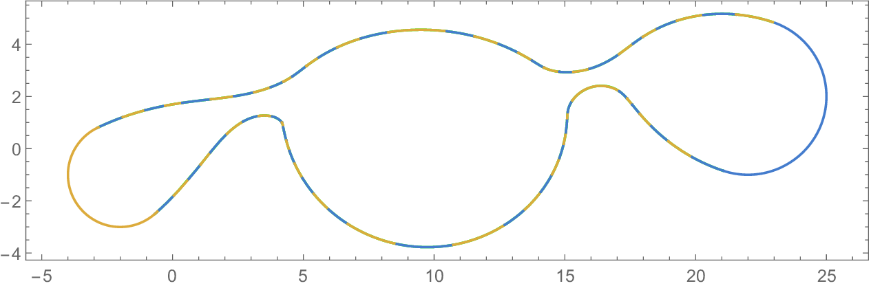
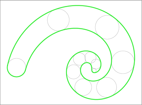
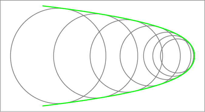
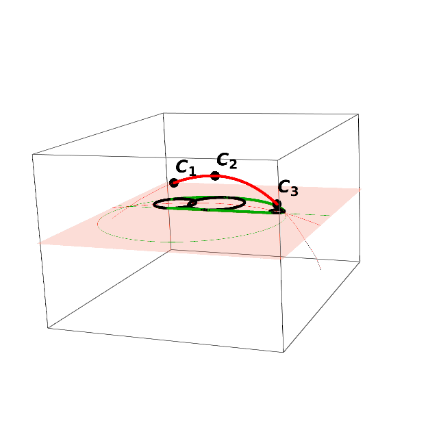
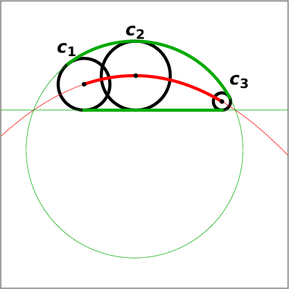
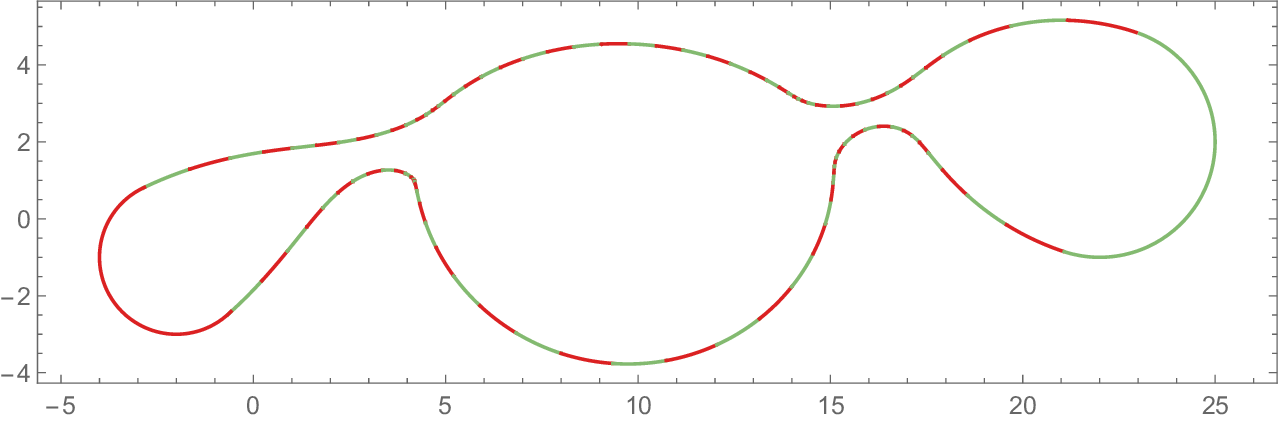
The envelope curves e ± C (u), u ∈ [a, b], (if they exist) and the cyclographic images of the endpoints C(a) and C(b) form a pre-boundary of the domain Ω. Its boundary δΩ is then a subset of the pre-boundary, obtained by trimming the self-intersections, see Figure 1.

Two planar oriented circles c 1 , c 2 are in oriented contact if they have a common point and share a tangent vector at this point. The corresponding points

A one parameter family of planar oriented circles that are all in oriented contact with two given oriented circles, defines a curve in the Minkowski space called a Minkowski circle. We extend this definition to more general situations. Furthermore, we review the rational parameterization for arcs of the Minkowski circles.

We consider the complex projective extension of Minkowski space R 2,1 . For a point C = (x, y, r) T ∈ R 2,1 , we introduce its homogeneous coordinates C = ( w : x : ȳ : r).

The absolute conic is defined as the set of points at infinity, i.e., points that satisfy the equations

A Minkowski circle C is a non-degenerate conic that shares two points (with multiplicity) with the absolute conic. The plane in which the Minkowski circle C lies determines its affine type. If the plane is

• space-like, C is an ellipse (a),

• time-like, C is a hyperbola with only space-like (b), or only time-like tangents (c),

• light-like, C is a parabola (d).

The envelope of the one parameter family of oriented circles given by the Minkowski circle C is composed of two oriented circles in the case (a) and (b), of an oriented circle and an oriented line, in the case (d), or, in the case (c), the family does not have a real envelope. Conversely, two oriented circles define a Minkowski circle of type (a) or (b). An oriented circle and an oriented line defines a Minkowski circle of type (d). A Minkowski circle is uniquely determined by three distinct points

, which define an arc on the Minkowski circle. We propose a quadratic parameterization of the Minkowski arc in the case when the difference vectors between the three points are not light-like.

be three points in the Minkowski space whose difference vectors are not light-like. Then

where

is the Minkowski arc interpolating C 1 , C 2 and C 3 .

Proof. We embed the points

and interpolate the points Ci , i = 1, 2, 3, by a Lagrange polynomial of degree 2 with the help of weights

Let PR denote the projectively extended real line. The curve Ã(u), u ∈ [0, 1], is a Minkowski arc if there are two points Ã(u 1 ), Ã(u 2 ) on the curve Ã(u), u ∈ PR, that lie on the absolute conic, i.e., the parameters u 1 , u 2 satisfy the equations

where the first one is of degree 4 and the second one of degree 2 in u. Hence there exist some q 0 , q 1 , q 2 ∈ R such that

Collecting the coefficients at u i , i = 0, 1, . . . , 4, produces a system of 5 equations, from which we eliminate the parameters q 0 , q 1 , q 2 . From the resulting equations we compute the weights a and b, where the only possible combination where both of them are non-zero is

which concludes the proof.

In [41] a quadratic rational Bézier parameterization of the Minkowski arc with three control points P 1 , P 2 , P 3 was suggested for the cases (a) and (b), when the Minkowski arcs have only space-like tangents. We propose an equivalent formulation.

Proposition 2. Let P 1 , P 2 , P 3 ∈ R 2,1 be three points in the Minkowski space such that ∥P 1 -P 3 ∥ M > 0 and ∥P 1 -P 2 ∥ M > 0 and ∥P 2 -

where

is the Minkowski arc satisfying

and

Proof. Following the same procedure as in the previous proof, we obtain the weight w. The weight is real and non-zero only if ∥P 1 -P 3 ∥ M > 0 and ∥P 1 -P 2 ∥ M > 0. The equations ( 7) and ( 8) follow from the properties of quadratic rational Bézier curves.

Next we consider biarcs in the Minkowski space. Given two points P 1 , P 2 ∈ R 2,1 and two unit space-like vectors t 1 , t 2 ,

we can construct a Minkowski biarc interpolating the data (P 1 , t 1 ) and (P 2 , t 2 ). The biarc consists of two Minkowski arcs A 1 j (u) and A 2 j (u), u ∈ [0, 1], that satisfies

and are joined continuously with continuous tangents,

We compute the Minkowski biarc following the construction from [41]. The biarc is given by 5 Bézier control points

where

i.e., the points P 1 , B 1 , J and J, B 2 , P 2 form isosceles triangles (with respect to the Minkowski inner product). The joint point J of the two Minkowski arcs is given by

Choosing the parameter λ 1 , equation (10) gives a unique parameter λ 2 . If λ 1 , λ 2 > 0, the joint point J lies between B 1 and B 2 and the Minkowski arcs lie inside of the triangles P 1 , B 1 , J and J, B 2 , P 2 . Furthermore, equation (10) ensures that the difference vectors J -B 1 and B 2 -J are space-like for any λ 1 ̸ = 0:

and hence

and similarly, ∥B 2 -J∥ M = λ 2 2 . Therefore, we can use Proposition 2 to parameterize the Minkowski biarc and its cyclographic image has a real envelope.

In this paper, we chose λ 1 > 0 such that

following the ’equal chord’ biarc interpolation scheme for planar data [38].

Minkowski arc splines are defined to be curves in Minkowski space R 2,1 composed of arcs of Minkowski circles.

Let C(u) = (x(u), y(u), r(u)) T , u ∈ [0, 1], be a Minkowski arc with only space-like (or isolated light-like) tangents. We note that the envelope of the one parameter family of circles defined by C(u) is formed by circular arcs or line segments. Two arcs are parts of the cyclographic images of the endpoints of the Minkowski arc. The other two arcs can be constructed as follows:

1. Let τ (u) be unit tangent vector at C(u),

2. For u * ∈ {0, 1}, we find the two light-like planes

For u * ∈ {0, 1}, we find the lines ℓ ± u * as the intersection of the planes ρ ± u * and the plane r = 0,

such that q ± u * ∈ R, ∥t ± u * ∥ = 1, and the lines ℓ ± u * (v) are in oriented contact with the circle ζ(C(u * )), i.e., their unit tangent vectors coincide at the common points. 4. For u * ∈ {0, 1}, we compute the points

where (t ± u * ) ⊥ denotes the vector (t ± u * ) rotated by π 2 counterclockwise. Those are exactly the envelope points e ± C (u * ) from equation (4). 5. The rotations mapping the pairs (p ± 0 , t ± 0 ) to the pairs (p ± 1 , t ± 1 ) define the envelope arcs.

We recall the medial axis and the medial axis transform of an open set Ω ⊂ R 2 . The boundary δD of a maximal disk is called a maximal circle.

In R 2 with the Euclidean metric, every maximal disk intersects δΩ in at least two points or it has a third order contact at points with stationary curvature. Definition 4. Let Ω be an open set in R 2 . The medial axis of Ω is the union of the centres of all maximal disks inscribed in Ω,

The medial axis transform MAT(Ω) of the set Ω also contains the information about radii of the maximal disks.

Let Ω be an open set in R 2 . The medial axis transform of Ω is defined as

We interpret the branches of MAT(Ω) as curves Note that if the branches B 1 (u), . . . , B n (u) of the MAT are Minkowski arcs, then Ω is an arc spline domain, i.e., a domain whose boundary is composed of circular arcs and line segments.

In this section, we introduce worms and evolving worms. We characterize the supersets of the envelopes of the evolving worms as the boundaries of cyclographic images of certain curves in the Minkowski space.

First, we define worms with the help of the cyclographic mapping: When a worm Ω evolves over time t and for each value of the time parameter its MAT is a single curve in R 2,1 , we call it an evolving worm. Definition 7. An evolving worm is a one-parameter family of planar domains Ω(t), t ∈ I t , such that for every t 0 ∈ I t the domain Ω(t 0 ) is a worm, i.e.,

The union of the preimages B t (u) of the evolving worms Ω(t) over the time parameters

Remark. We can define a strong evolving worm to be a one-parameter family of planar domains Ω(t), t ∈ I t , such that for every t 0 ∈ I t the domain Ω(t 0 ) is a strong worm, i.e.,

The union of the medial axis transforms of the strong evolving worms is again a surface in Minkowski space R 2,1 ,

The envelope of the evolving worm Ω(t), t ∈ [0, 1], is the envelope of a two-parameter family of oriented planar circles. If B(u, t) = (x(u, t), y(u, t), r(u, t)) T , u, t ∈ [0, 1] , the circles are centred at (x(u, t), y(u, t)) T and their radii are given by the function r(u, t).

We characterize the envelope of an evolving worm. Let Ω(t), t ∈ [0, 1], be an evolving worm represented by a smooth surface B(u, t) in Minkowski space R 2,1 . B(u, t) = (x(u, t), y(u, t), r(u, t)) T , u, t ∈ [0, 1] .

We identify singular curves on the surface B(u, t). The cyclographic images of the singular curves contribute to the envelope of the evolving worm. Definition 8. Let B(u, t), u, t ∈ [0, 1], be a surface in Minkowski space R 2,1 . A point B(u 0 , t 0 ), u 0 , t 0 ∈ [0, 1], is a singular point of B(u, t), if the vectors v u (u 0 , t 0 ) = ∂B(u, t) ∂u u=u 0 ,t=t 0 and v t (u 0 , t 0 ) = ∂B(u, t) ∂t u=u 0 ,t=t 0 are either linearly dependent or if they span a light-like plane.

Let u 0 , t 0 ∈ [0, 1]. The restriction of the quadratic form defined by G = diag(1, 1, -1) on the tangent plane to B(u, t) at the point B(u 0 , t 0 ) is defined by the 2 × 2 matrix

where v u = v u (u 0 , t 0 ) and v t = v t (u 0 , t 0 ).

The tangent plane is light-like if the quadratic form M (u 0 , t 0 ) is indefinite degenerate, that is, det(M (u 0 , t 0 )) = 0 .

Equation ( 13) identifies the points of the surface B(u, t) with light-like tangent planes as well as the second type of the singular points from Definition 8, i.e., the points where the tangent plane is not defined. If B(u, t) is piecewise rational surface, Equation ( 13) defines an algebraic curve in the parameter domain. Points B(u 0 , t 0 ) for u 0 , t 0 ∈ [0, 1], that satisfy Equation ( 13) then form the singular curves on the surface B(u, t).

The envelope of the evolving worm Ω(t) then consists of boundaries of the cyclographic images of the singular curves and the boundary curves of the surface B(u, t). This fact was noted in [42]. Here we present a formal proof.

Theorem 3. The envelope of an evolving worm Ω(t), t ∈ [0, 1], given by the surface

is a subset of the cyclographic images of the boundary curves

and of the cyclographic images of the singular curves.

Proof. We denote B(u, t) = (x(u, t), y(u, t), r(u, t)), u, t ∈ [0, 1]. The surface defines a two parameter family of planar circles p, which can be parameterized with the help of three parameters u, t ∈ [0, 1] and φ ∈ [0, 2π), p(u, t, φ) =

x(u, t) y(u, t) + r(u, t) cos φ sin φ .

The boundary curves correspond to the families of circles

and the cyclographic images of the boundary curves are envelopes of these families of circles, that clearly correspond to the envelope of Ω(t). Let u, t ∈ (0, 1). Any point of the envelope of the two parameter family of circles p(u, t, φ) satisfies the envelope condition (see e.g. [42] Eliminating the parameter φ from the equations above yields the equation

which is exactly the equation ( 13) multiplied by -r. Hence we see that the points that satisfy the envelope condition are the points of the cyclographic images of the singular points and the circles of the two parameter family which have zero radii.

The envelope of an evolving worm consists of boundaries of cyclographic images of certain curves in R 2,1 . We present and compare two pairs of methods for curve interpolation in the Minkowski space by Minkowski arcs either directly, or indirectly, by interpolating the boundaries of the cyclographic images of the original curves. In both cases, we interpolate the curve or the boundary of its cyclographic image either by (Minkowski) arcs or (Minkowski) biarcs. The resulting envelope of the evolving worm is then an arc spline.

We consider curves with space-like tangents only. Light-like tangents may be present at endpoints. The four schemes described below need to be modified to deal with these points. This is described in the appendix of the paper.

Let Ω ⊂ R 2 be a worm and let

The direct methods interpolate the curve C(v) by Minkowski (bi)arcs. The boundaries of the cyclographic images of interpolants are composed of circular arcs and approximate the boundary δΩ. The MAT of the approximated worm is an Minkowski arc spline. We assume that the curve C(v) has only space-like or isolated light-like tangents, i.e., the worm Ω is the cyclographic image of the whole curve C(v).

We choose N ∈ N and sample points on the curve

and denote the samples

We interpolate segments of the curve C(v) by Minkowski arcs (direct arc interpolation, DAI), or by Minkowski biarcs (direct biarc interpolation, DBI). Then we compute the boundaries of the cyclographic images of the Minkowski (bi)arcs exactly. These curves are composed of circular arcs and approximate the boundary of the worm Ω.

We interpolate segments of the curve C(v), v ∈ [0, 1], in Minkowski space R 2,1 by Minkowski arcs and approximate the boundary of the worm Ω by the boundaries of the cyclographic images of the Minkowski arcs. 1 with only space-like or isolated light-like tangents, N ∈ N even. Output: Superset of the boundary of the domain Ω that approximates the worm Ω,

The boundary of the domain Ω is a subset of the boundaries of the cyclographic images,

The approximated worm Ω is then a cyclographic image of the Minkowski arc spline

where

However, the endpoints of the envelope curves of two consecutive segments Ck (v) and Ck+1 (v) do not generally coincide. Therefore we need to include also the cyclographic images of the endpoints C k (0) and C k (1) of the Minkowski arc spline segments Ck (v), v ∈ [0, 1], for k = 1, . . . , N -1 2 , to approximate the whole boundary of the worm Ω.

We interpolate segments of the curve C(v), v ∈ [0, 1], in Minkowski space R 2,1 by Minkowski biarcs and approximate the boundary of the worm Ω by the boundaries of the cyclographic images of the Minkowski biarcs. 1 with only space-like or isolated light-like tangents, N ∈ N. Output: Superset of the boundary of the domain Ω that approximates the worm Ω,

At each point C j , j = 0, 1, . . . , N , compute the normalized tangent vector t j of the curve C(v),

4. For each j = 0, 1, . . . , N -1, we compute the control points of a Minkowski biarc that interpolates the consecutive pairs of data

and parameterize the arcs of the biarc Cj (v), v ∈ [0, 1], according to Proposition 2.

For each j = 0, 1, . . . , N -1 we compute the envelope curve

6. The boundary of the domain Ω is a subset of the envelope curves and arcs of the cyclographic images of C 0 and C N ,

Note that as we assume all the tangents of the curve C(v), v ∈ [0, 1], to be space-like, we can always normalize them.

The approximated worm Ω is then a cyclographic image of the Minkowski arc spline

where j = 0, 1, . . . , N -1. The Minkowski arc spline is G 1 continuous and the envelope curves e ± C (v), v ∈ [0, 1], are planar circular arc splines and are C 1 continuous at the points C j for j = 2, . . . , N -1.

Let Ω ⊂ R 2 be a worm and let C(v), v ∈ [0, 1], be a curve in Minkowski space R 2,1 such that

The indirect methods interpolate the boundary δΩ, more specifically the envelope curves e ± C , by planar circular (bi)arcs. The approximated worm is then a cyclographic image of a geometric graph in R 2,1 , which has Minkowski arcs as its branches.

We assume that the curve C(v) has only space-like or isolated light-like tangents. Furthermore, we assume that the envelope curves e ± C (v), v ∈ [0, 1], do not have any singular points.

We choose N ∈ N and sample the curve

and we compute the corresponding envelope points e ± j = e ± (v j ), j = 0, . . . , N .

We interpolate the envelope points by planar circular arcs (indirect arc interpolation, IAI), or planar biarcs (indirect biarc interpolation, IBI). These curves form the boundary δ Ω of the domain Ω which approximates the worm Ω.

The arc spline δ Ω approximates the boundary δΩ with approximation order 3, see [38].

We interpolate segments of the envelope curves e ± C (v) of the curve C(v), v ∈ [0, 1], by planar circular arcs. 1 with only space-like or isolated light-like tangents, such that e ± C (v), v ∈ [0, 1], has no singular points, N ∈ N even. Output: Superset of the boundary of the domain Ω that approximates the worm Ω,

For each j = 0, 1, . . . N , compute the envelope points e ± j = e ± (v j ), j = 0, . . . , N .

For each k = 0, 1, . . . , N 2 -1, interpolate the three consecutive points e + 2k , e + 2k+1 , e + 2k+2 , by a planar circular arc ẽ+

The boundary of the domain Ω is a subset of the envelope curves ẽ± k (v), v ∈ [0, 1], and arcs of the cyclographic images of C 0 = C(0) and

The arc splines

where k = 0, 1, . . . , N 2 -1, are C 0 continuous at the points e ± 2k+1 , k = 1, . . . , N -3 2 . The MAT of the domain Ω is a geometric graph whose branches are Minkowski arcs.

We interpolate segments of the envelope curves e ± (v) of the curve 1 with only space-like or isolated light-like tangents, such that e ± C (v), v ∈ [0, 1] has no singular points, N ∈ N even. Output: Superset of the boundary of the domain Ω that approximates the worm Ω,

For each j = 0, 1, . . . N , compute the envelope points e ± j = e ± (v j ), j = 0, . . . , N .

For each j = 0, 1, . . . , N, compute the unit tangent vectors t ± j of the envelope curves e ± C (v) at the points e ± j . 4. For every j = 0, 1, . . . , N, compute biarcs ẽ± j (v), v ∈ [0, 1], interpolating the pairs e ± j , t ± j and e ± j+1 , t ± j+1 .

The boundary of the domain Ω is a subset of the envelope curves ẽ± j (v), v ∈ [0, 1], and arcs of the cyclographic images of C 0 = C(0) and

The arc splines

where k = 0, 1, . . . , N -1, are G 1 continuous In general, the MAT of the domain Ω is a geometric graph with Minkowski arcs as branches.

We compare the four methods DAI, DBI, IAI, and IBI for the approximation of the boundary of the worm Ω whose MAT is represented by a curve C(v), v ∈ [0, 1], with respect to the number of arcs, approximation power and continuity. The results are summarized in Table 1.

Let N ∈ N be and even number. We sample the interval [0, 1] uniformly and N + 1 parameter values and denote h = 1 N .

The methods described above return the superset of the arcs that approximate the boundary of worm Ω. These arcs are the input for the sweep line algorithm that extracts the real envelope. We compare the cardinality of the supersets, which gives an upper bound of the number of arc in the approximated boundary.

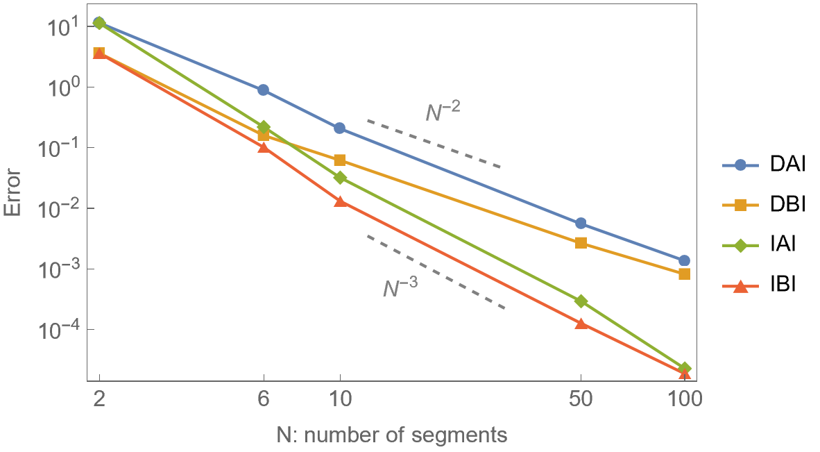
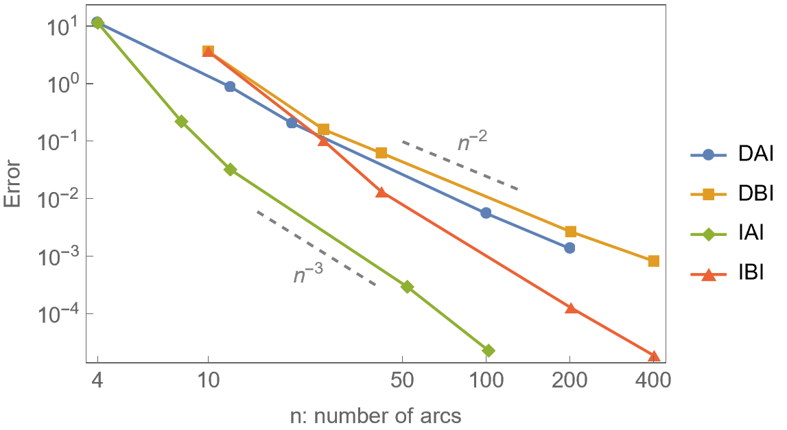
The indirect methods IAI and IBI approximate the boundary of the worm Ω with approximation order 3. The direct methods DAI and DBI approximate the boundary only with approximation order 2. We consider the error with respect to the number of segments, or number of arcs (Figure 6, right). Among the methods considered, the IAI method generates the lowest number of arcs for a given accuracy.

Ω Regarding the continuity, the boundary δ Ω is C 0 continuous for the methods DAI and IAI and C 1 continuous in the case of the methods DBI and IBI. In summary, when deciding which method to use, we can follow the quidelines outlined here:

• IBI offers the best option when C 1 smoothness is desired.

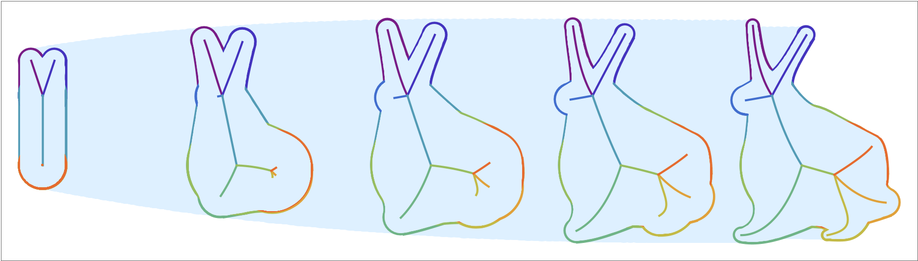
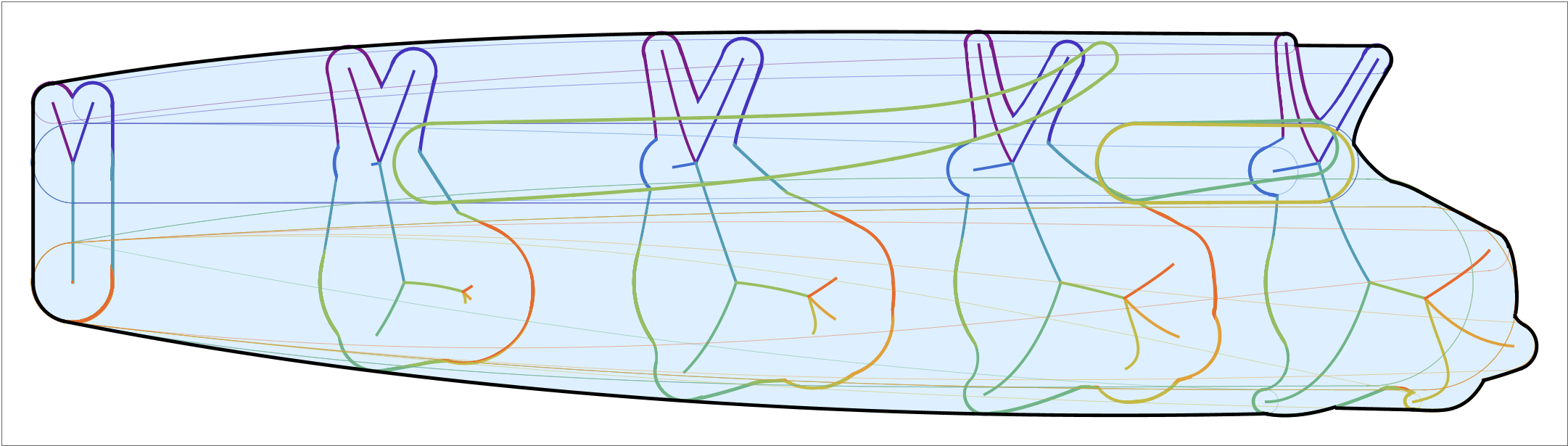
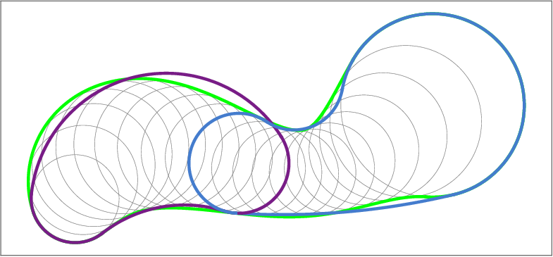
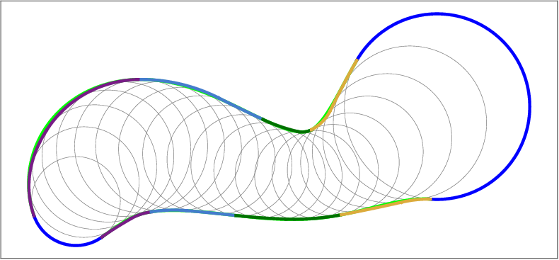
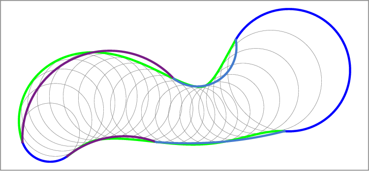
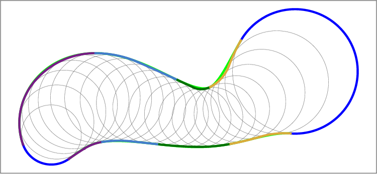
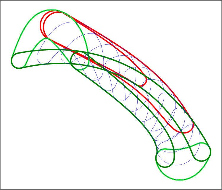
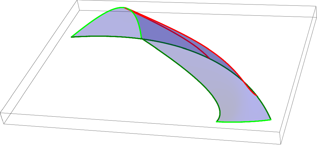
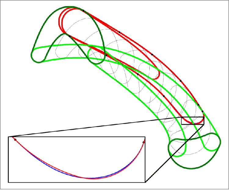
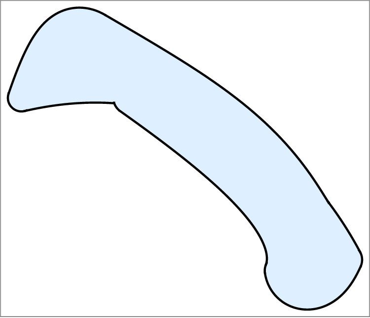
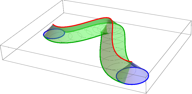
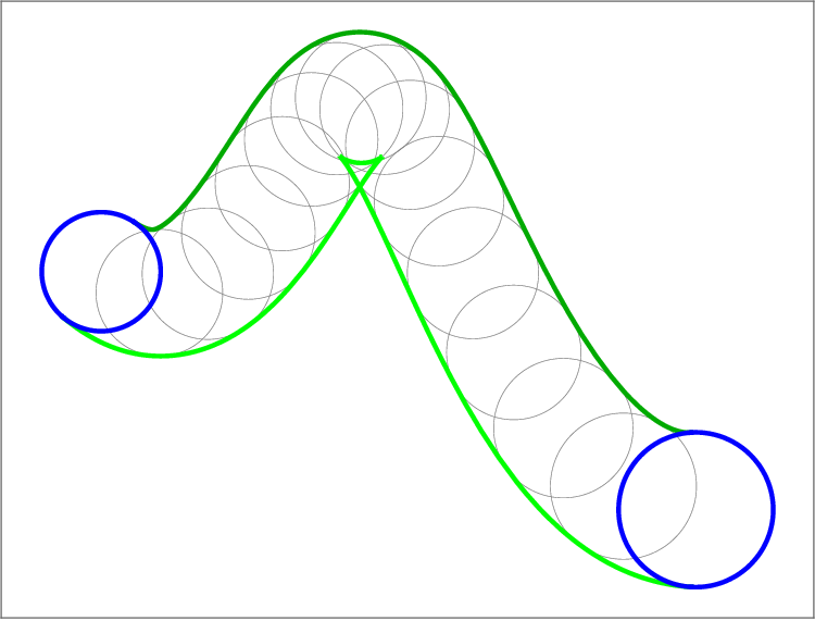
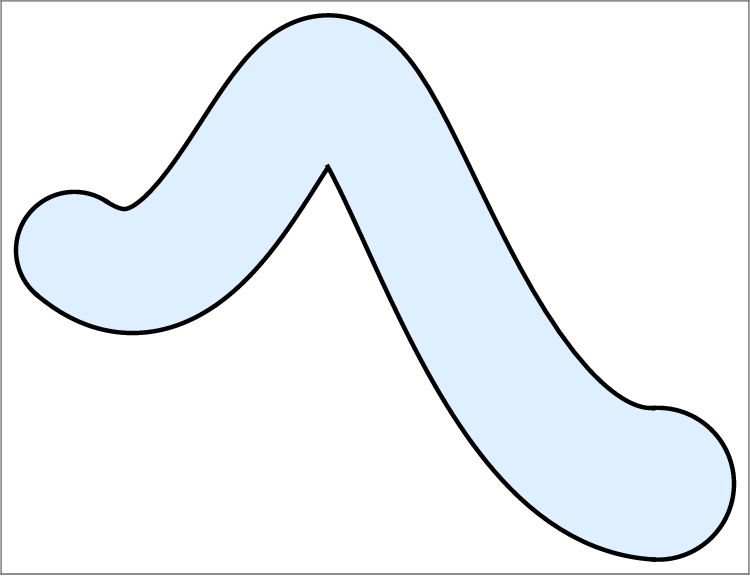
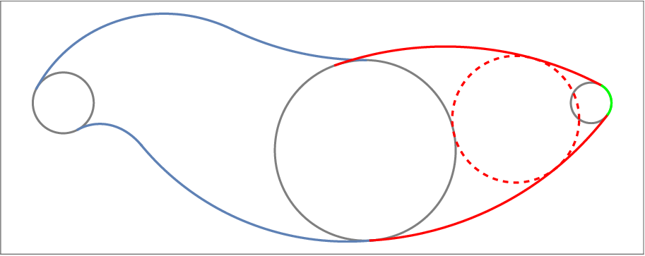
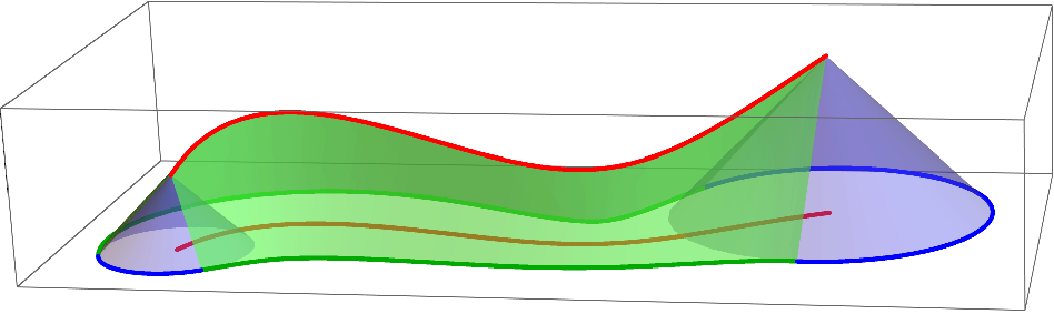
• IAI produces the lowest number of arcs for a given precission. The approximation of the evolving worm using the method IBI and N = 4 (centre). The boundaries of the cyclographic images of the boundary curves B(u, 0), B(u, 1), the boundary curves B(0, t), B(1, t) and the singular curves are depicted in blue, their approximations in light green, dark green and red, respectively. The envelope of the evolving domain is a subset of the boundaries of the cyclographic images (right).

In this section we describe the computation of the envelope of an evolving worm using one of the four method presented above.

Let Ω(u, t), u, t ∈ [0, 1], be an evolving worm defined by a piecewise smooth rational surface B(u, t), u, t ∈ [0, 1], in Minkowski space R 2,1 . By Theorem 3 we know that the envelope of Ω(u, t) is a subset of the boundaries of the cyclographic images of the boundary and the singular curves on the surface B(u, t). To approximate the boundary curves, can we simply use one of the methods DAI, DBI, IAI or IBI for the curves

The singular curves are defined by Equation (13). The equation defines an algebraic curve in the parameter domain. Adapting a method for tracing algebraic curves from [34], we trace points (u i , t i ) T on the curve in the parameter domain and tangent vectors v i = (v i u , v i t ) T at those points. From this data, we recover the singular points p i = B(u i , t i ) T on the surface B(u, t) and tangent vectors

We divide the singular curves into segments with space-like, light-like and time-like tangents and only consider those with space-like tangents and possibly light-like tangents at the endpoints. The segments with time-like tangents do not correspond to a real envelope and hence we do not need to consider them further.

To approximate the singular curve using the method DAI, we only need the points p i . For the other methods, we also need the tangent vectors τ i . For the method IBI, the tangent vectors t i of the envelope points are also necessary, see Equations ( 11) and ( 12) for the construction of the tangent vectors and the envelope points.

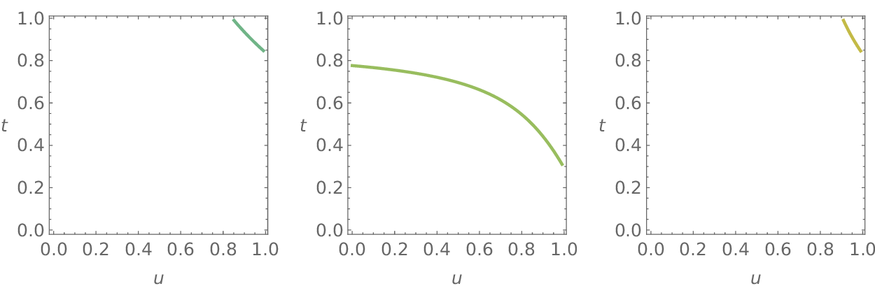
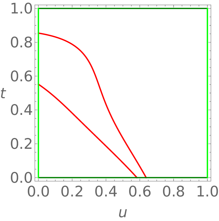
Figure 8 (left) shows the singular and the boundary curves on the surface B(u, t) depicted in Figure 4 in the parameter domain. We sampled 5 points on the curves and computed the Hermite data on the envelope curves to approximate the envelope of the envelope of the evolving worm using the method IBI. The outer envelope can be extracted after computing intersections of the biarcs using a line sweep algorithm, see Figure 8 (right).

We apply the developed method for computation of envelopes of evolving worm to evolving free-form domains.

We interpret a free-form domain Ω ⊂ R 2 as a union of worms, e.g., the cyclographic images of the branches of the MAT(Ω). Let B 1 (u), . . . , B n (u) for some n ∈ N and u ∈ [0, 1] be curves in Minkowski space R 2,1 ,

and the domain Ω is the union of the worms

A free-form domain Ω(t) evolving in time t ∈ [0, 1], is then represented as a union of evolving worms. Each of the evolving worms B 1 (u, t), . . . , B n (u, t) , We approximate each evolving branch separately, by approximating the worms corresponding to the boundary and the singular curves of each of the surfaces B i (u, t) , i = 1, . . . , 9 .

In this example, the only evolving worms with singular curves are those shown in dark green, light green and yellow (see Figure 10a and10b). We approximate the boundaries of the cyclographic images of the singular curves and of the boundary curves using the method IBI. In this case, the cyclographic images of the singular curves do not contribute to the envelope of the evolving domain and are trimmed away. The envelope of the evolving domain is then extracted from the interpolations of the cyclographic images of the boundary curves.

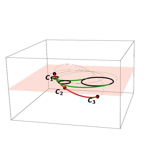
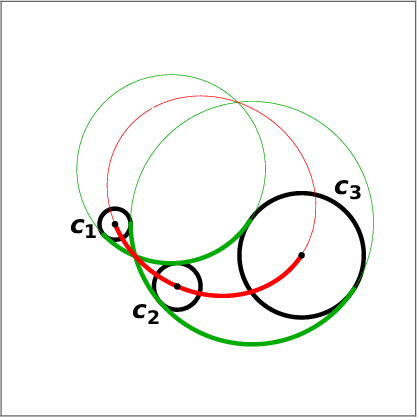
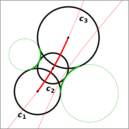
Example 2. Let Ω(t), t ∈ [0, 1] be the evolving domain shown in Figure 11a. At each time instance, the domain is a union of three worms. In this case, the MAT of each worm has a non-zero length at each time parameter.

We approximate every evolving branch separately. For each i = 1, 2, 3, we identify the (11a) Evolving planar domain Ω(t). At every t ∈ [0, 1] it consists of three worms.

(11b) The outer envelope of Ω(t).

(11c) The superset of the envelope consists of boundaries of cyclographic images of both the singular (thick) and the boundary curves. and approximate the corresponding worms using the method IBI. The cyclographic images of the singular curves are necessary to approximate the envelope of the evolving domain, approximately 32 % of the envelope arcs are contributed by the singular curves. Figure 11c shows the superset of the envelope with highlighted cyclograpic images of the singular curves and Figure 11b depicts the extracted outer envelope, where the arcs contributed by the singular curves are highlighted.

Example 3. The presented method allows us to compute envelopes of evolving domains, where the number of components changes. The domain in Figure 12a is composed of two worms at each instance of the time parameter. At the beginning, the worms are connected, and as the domain evolves, they separate, creating two components. We identify the boundary and the singular curves on both surfaces in the Minkowski space and again use the method IBI to approximate the envelope. Figure 12b shows the boundaries of the cyclographic images of the boundary curves of the both worms. To obtain the whole envelope, we also need to consider the singular curves. Figure 12c shows the extracted envelope of the evolving domain, where the boundaries of the cyclographic images of the singular curves of both worms are highlighted. In this example, approximately 14 % of the envelope arcs are contributed by the singular curves.

We presented a procedure for approximating the envelope of planar domains that evolve in time. First, we considered worms, which are cyclographic images of single curve seg-29 ments in R 2,1 . We characterized the envelopes of evolving worms as subsets of cyclographic images of finitely many curves in Minkowski space. We then proposed two pairs of methods to approximate these curves and their cyclographic images by arc splines. The methods exploit geometric flexibility and computational simplicity of circular arcs to efficiently and precisely approximate the envelopes. We considered free-form domains to be unions of worms. Finally, the envelope of an evolving (free-form) domain was obtained by trimming the redundant curves efficiently using a line sweep algorithm that again utilized the properties of circular arcs.

In Section 4, we presented four methods for approximation curves in the Minkowski space R 2,1 and their cyclographic images. We only considered curves with space-like tangents, however, light-like tangents may be present at endpoints. Figure 13 shows such a situation.

We discuss the effect of these points for the four methods:

• DAI: The method can be applied without any problems. The arcs of the circles that correspond to the endpoints must be added to the envelope. • DBI: The method cannot be used if one of the segment end points has a light-like tangent. Let v N = 1 be the last parameter value, such that the tangent at the point C N = C(v N ) is light-like, i.e., ∥C(v N ) ′ ∥ M = 0. We sample one additional point on the curve C(v),

and we use a single Minkowski arc that interpolates the points C N -1 , C N - , C N to represent the last segment. See Figure 14 for an illsutration.

• IAI: The method can be used, however a reparameterization of the boundary curve is needed since the parametric speed tends to infinity as we approach the point with a light-like tangent, which corresponds to a vertex of the boundary curve.

• IBI: The method can also be used, again after performing a reparameterization of the boundary.