Beyond Binary Classification: A Semi-supervised Approach to Generalized AI-generated Image Detection

To address this generalization gap, the fundamental challenge lies in understanding why different architectural families produce systematically different patterns. Prior research has primarily explored that GANs and DMs leave surfacelevel artifacts in synthetic images, such as checkerboard patterns (Dzanic, Shah, and Witherden 2020;Zhang, Karaman, and Chang 2019;Frank et al. 2020;Wang et al. 2020a) and noise residuals (Wang et al. 2023;Ma et al. 2024). However, this approach faces an inherent limitation: these surfacelevel artifacts are vulnerable to simple post-processing operations, further limiting detection robustness. In contrast to prior work, we shift from analyzing surface-level artifacts to latent architectural patterns inherent to each generative architecture family. Specifically, we hypothesize that latent representations of synthetic images generated by GANs and DMs form significantly different submanifolds in feature space. This hypothesis stems from the fundamental observation that GANs and DMs have distinct optimization objectives, which fundamentally shape how these generative architecture families model data distribution: the Jensen-Shannon (JS) divergence is optimized by GANs, whereas the Kullback-Leibler (KL) divergence is minimized by DMs.

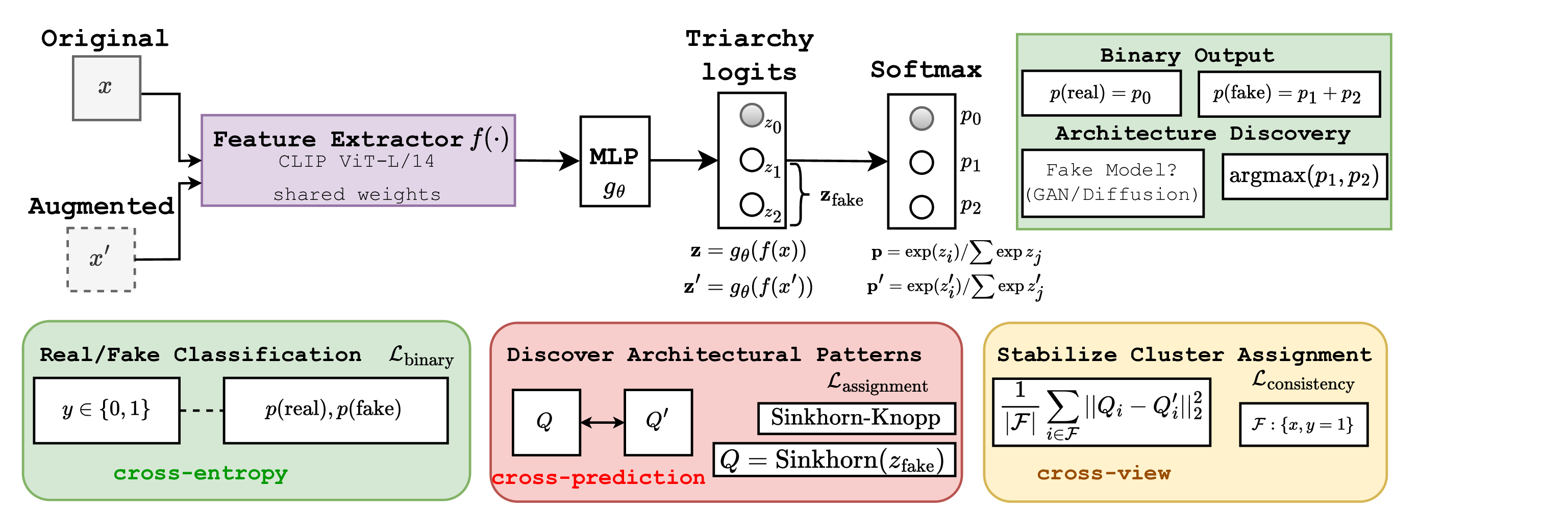
In this work, we demonstrate the existence of latent architectural patterns inherent to each generative architecture family (i.e., GANs and DMs) through a theoretical analysis of their optimization objectives. By utilizing the manifold hypothesis (Fefferman, Mitter, and Narayanan 2016;Loaiza-Ganem et al. 2024), we show that GANs and DMs interact with the data manifold differently: GANs permit partial manifold coverage, leading to boundary artifacts, while DMs enforce complete coverage, resulting in oversmoothing patterns. This theoretical disparity implies that GAN-generated and DM-generated images occupy distinct, separable submanifolds within a well-learned feature space (Fig. 2). This theoretical analysis directly guides our method design. Rather than attempting to detect specific generators or relying on surface-level patterns, we propose Triarchy Detector (TriDetect), a novel semi-supervised method designed to recognize these fundamental architectural signatures. Specifically, TriDect simultaneously performs binary classification while discovering latent architectural pat- terns within the synthetic data (Fig. 1). To ensure robust learning, we employ the Sinkhorn-Knopp algorithm (Cuturi 2013) to enforce balanced cluster assignments, preventing cluster collapse. Furthermore, a cross-view consistency mechanism is designed to ensure the model learns fundamental architectural distinctions rather than image statistics. By discovering latent architectural patterns, our method can enhance the cross-generator generalization within the same architecture families.

Main Contributions. Our contributions include:

• Theoretical Analysis: We provide the first theoretical explanation for why the GAN and DM architectures produce fundamentally different latent patterns, grounded in their optimization objectives and manifold coverage.

• Novel Semi-supervised Detection Method: We introduce TriDetect that combines binary classification with architecture-aware clustering to learn generalized architectural features.

• Comprehensive Evaluation: We evaluate on 5 datasets against 13 SoTA detectors, demonstrating superior crossgenerator and cross-dataset generalization.

In this section, we provide the theoretical analysis to demonstrate that latent representations of synthetic images generated by GANs and DMs form significantly different submanifolds in feature space. The t-SNE visualization in Figure 2 confirms this analysis. Specifically, our analysis reveals that these differences are fundamental consequences of their optimization targets. We begin by examining the optimization objectives of each architecture family, then demonstrate how these objectives lead to characteristic coverage patterns and to distinguishable artifacts.

We use p data , p GAN , and p DM to denote the data, GANgenerated, and DM-generated distributions, respectively. Lemma 1. (DM Optimization Objective). Suppose that x 0 ∼ p data , DM minimizes an upper bound on the KL divergence between the data and model distributions:

where ELBO is the Evidence Lower Bound and H(p data ) is the entropy of the data distribution.

Remark 1. (Equality Condition). The inequality in Lemma 1 becomes an equality when the variational posterior q(x 1:T |x 0 ) equals the true posterior p DM (x 1:T |x 0 ) under the model. In standard DMs, this condition can be achieved at the global optimum when the reverse process has sufficient capacity (Luo 2022), yielding:

Lemma 1 is supported by recent works on DMs (Luo 2022;Nichol and Dhariwal 2021), which indicates that DMs indirectly minimize the KL divergence by maximizing the ELBO. KL divergence is asymmetric and severely penalizes the model if p DM = 0 where p data > 0.

Lemma 2. (GAN optimization problem) For a fixed generator G, the value function V (D, G) satisfies the inequality:

with equality if and only if the discriminator is optimal, given by D * (x) = p data (x)/(p data (x) + p GAN (x))

In contrast to DMs, GANs optimize the JS divergence through an adversarial game (Che et al. 2020;Goodfellow et al. 2020;Arjovsky, Chintala, and Bottou 2017). Unlike the KL divergence, the JS divergence is symmetric and remains bounded even when the generator completely ignores certain regions of the data space.

These lemmas lead to our first key theoretical result:

The choice of divergence profoundly impacts the learned distributions and the nature of artifacts inherent to the generation process.

Theorem 2. (Disparity of Learned Distribution Support) Let p data be the true data distribution with support S data = {x : p data (x) > 0}. Assume that the generator and scorematching networks have sufficient capacity:

1. GANs: A globally optimal solution for the GAN generator, which minimizes the JS divergence D JS (p data ∥p GAN ), can exist even if the support of the learned distribution, S GAN , is a strict subset of the data support (S GAN ⊂ S data , partial coverage).

2. DMs: A globally optimal solution for the DM, which minimizes the upper bound on the KL divergence D KL (p data ∥p DM ), requires the support of the learned distribution, S DM , to cover the support of the data distribution (S data ⊆ S DM , complete coverage).

Proof in Appendix. Theorem 2 reveals why GANs and DMs exhibit fundamentally different coverage behaviors. For DMs, to achieve an optimal solution, the support of its learned distribution must cover the support of the real data distribution (S data ⊆ S DM ). This is because the KL divergence D KL (p data ∥p DM ) becomes infinite whenever p DM = 0 for any x where p data > 0. As a result, DMs must spread their capacity across the entire data manifold, resulting in diffusion blur, over-smoothing in low-density regions. Furthermore, the iterative denoising process of DMs relies on score matching. Imperfections in this estimation accumulate during the reverse diffusion steps, combined with the smoothing enforced by the KL objective, will leave unique, structured noise residuals that serve as a distinct architectural artifact (Wang et al. 2023;Ma et al. 2024). In contrast, due to JS divergence optimization, GANs can achieve optimality while ignoring low-probability regions of p data . This leads to sharp samples but incomplete coverage where GANs concentrate their capacity on high-density modes, producing sharp samples but missing rare patterns. The boundary artifacts manifest as abrupt transitions at the edges of learned support, creating detectable discontinuities. These discontinuities manifest in the image space as characteristic boundary artifacts, such as structural inconsistencies or unnatural texture transitions (Zhang, Karaman, and Chang 2019).

This section presents a semi-supervised Trirchy Detector (TriDetect) that simultaneously performs binary classification and discovers latent structures within synthetic images. From our theoretical analysis, by learning to recognize distinct architectural patterns that persist across specific generators within each family (i.e., GANs vs. DMs), it is possible to achieve cross-generator generalization capability.

Given a dataset D = {(x i , y i )} N i=1 where x i ∈ R H×W ×3 represents an image and y i ∈ {0, 1} denotes its binary label (0:real, 1:fake), we compute logits z i = g θ (f (x i )) ∈ R 3 using a fine-tuned vision encoder f and classifier g θ , where we have 3 output dimensions (one real class and two fake clusters). We formulate a joint optimization problem with two objectives: (i) distinguish real from synthetic images, and (ii) automatically discover latent clusters within synthetic samples that correspond to different generative architectures. The architecture produces three-way logits that align with the theoretical distinction between GAN and DM architectures established in our analysis.

A critical challenge in unsupervised deep clustering is the tendency toward trivial solutions where all samples collapse into a single cluster (Zhou et al. 2024). This problem is particularly serious in our setting, where we seek to discover subtle architectural patterns within synthetic images generated by different generators. To address this, we formulate cluster assignment as an optimal transport problem that enforces balanced distribution across clusters.

For a batch B of synthetic samples with logits Z fake ∈ R B×K where K = 2 is the number of fake clusters, we seek an assignment matrix Q ∈ R B×K that maximizes the similarity between samples and clusters while maintaining balanced assignments:

where

These constraints ensure that each sample is fully assigned across clusters (rows sum to 1) and each cluster receives exactly B/K samples (columns sum to B/K), preventing collapse.

Sinkhorn-Knopp Algorithm for Online Clustering. We utilize the Sinkhorn-Knopp algorithm (Cuturi 2013) to solve the optimal transport problem. Starting from the initialization Q (0) = exp(Z fake /ϵ), for t = 1, . . . , T iterations, we perform:

where

k Q kj normalizes columns with appropriate scaling to maintain the balance constraints. Note that Eq. 6 is operated on mini-batches rather than the entire dataset, enabling online learning that scales to arbitrarily large datasets.

To learn discriminative and generalized clusters that capture architectural patterns rather than image statistics, we propose a cross-view consistency mechanism that encourages consistent predictions and clustering stability. This mechanism contains the swapped prediction strategy and consistency regularization.

Swapped Prediction for Cluster Learning. Let (x, x ′ ) denote different views, generated by random transformations on each image, with corresponding logits (z, z ′ ). For fake samples, we extract the fake cluster logits z fake and z ′ fake . Inspired by the work (Caron et al. 2020), the core idea here is to use the cluster assignment from one view to supervise the prediction from the other view. Specifically, after computing balanced assignments using the Sinkhorn-Knopp algorithm Q = Sinkhorn(z fake ) and Q ′ = Sinkhorn(z ′ fake ) for fake samples in each view, the assignment loss is computed as follows:

Qfake, Q ′ fake ← Sinkhorn(Zfake), Sinkhorn(Z ′ fake ) ▷ Balanced assignment 9:

Compute Lbinary (Eq.10), Lassignment (Eq.7), Lconsistency (Eq.8) 10:

Lcluster ← ω1Lassignment + ω2Lconsistency 11:

Ltotal ← βLbinary + (1 -β)Lcluster 12:

θ ← θ -η∇ θ Ltotal ▷ Update parameters 13:

end for 14: end for 15: return f, g θ where F denotes the set of fake samples in the batch and p ik = exp(z ik /τ ) j exp(zij /τ ) with temperature τ . Consistency Regularization for Stable Assignments. The consistency regularization ensures that the Sinkhorn-Knopp assignments themselves remain stable across views, preventing oscillation during training and encouraging convergence to meaningful clusters. Particularly, this additional regularization directly constrains the similarity of assignments themselves:

The overall loss function for training TriDetect contains the binary classification loss and the clustering loss:

where L cluster = ω 1 L assignment + ω 2 L consistency . β denotes the hyperparameter that balances the importance of the binary and clustering losses while ω 1 and ω 2 represent assignment and consistency weights. L binary is the cross-entropy loss, computed as:

(10) where p i = softmax(z i ) ∈ R 3 , with p(real) i = p i,0 and p(fake) i = p i,1 + p i,2 . We provide the training pseudocode in Alg. 1 and the Sinkhorn-Knopp algorithm in Appendix. Datasets. We evaluate our method on 2 standard benchmarks (GenImage (Zhu et al. 2023), AIGCDetectBenchmark (Zhong et al. 2023)) and 3 in-the-wild datasets (Wild-Fake (Hong et al. 2025), Chameleon (Shilin et al. 2025), DF40 (Yan et al. 2024)). In our experiments, we follow the training protocol introduced by (Shilin et al. 2025) by utilizing BigGAN and SDv1.4 subsets of GenImage.

Metrics. In this work, we report results across 4 commonly used metrics: accuracy (ACC), area under the ROC curve (AUC), equal error rate (EER), and average precision (AP). We primarily report AUC and ACC in the main paper; other metric results are provided in Appendix.

Implementation Details. We use CLIP ViT-L/14 (Radford et al. 2021) vision encoder f , which is fine-tuned with Low-Rank Adaptation (LoRA) (Hu et al. 2022). For baseline implementation, we use two benchmarks, DeepfakeBench (Yan et al. 2023) and AIGCDetectBenchmark (Zhong et al. 2023). Detailed experimental procedures, hyperparameters, and configurations are provided in Appendix.

Standard Benchmarks. On GenImage, Table 1 shows that TriDetect achieves the highest average AUC of 0.9882, outperforming SoTA methods, including AIDE (0.9152), NPR (0.9695), and Effort (0.9815). The results on AIGCDe- tectBenchmark (Table 2) also demonstrate the generalization capability of TriDetect to 16 unseen generators, yielding an improvement over DIRE (22.18%), AIDE (17.4%), UnivFD (5.6%), NPR (6.5%), and Effort (0.9%).

In-the-wild Datasets. Tables 345show that our method outperforms existing detectors across all evaluation metrics on in-the-wild datasets:

• Robust to degradation techniques: TriDetect exhibits consistent performance when evaluated on WildFake in which degradation techniques (e.g., downsampling, cropping) are applied on testing sets. Particularly, TriDetect achieves an average ACC of 0.8254, a 8.86% improvement compared to Effort. Results demonstrate the better robustness of TriDetect than other methods. • Generalize to facial editing methods: On DF40 dataset, TriDetect achieves an average ACC of 0.8429, an improvement of 3.08% and 29.43% compared to Effort and UnivFD, respectively.

• Achieve lowest EER: On the challenging Chameleon dataset (Table 5), which is designed to deceive both humans and AI models, TriDetect attains the lowest EER of 0.1843, a 31.74% reduction compared to Effort. This demonstrates that our approach can achieve a superior balance between false positive and false negative rates.

The ablation study on β (Table 7) reveals a crucial insight: the optimal balance between binary classification and clustering objectives occurs at β = 0.7, where the model achieves peak performance across all metrics.

Figure 2 provides visual evidence that TriDetect successfully discovers meaningful latent structure within synthetic images. The alignment between unsupervised discovery (left figure) and ground truth (right figure) validates our theoretical analysis that different generative architectures leave distinguishable artifacts in feature space. The middle figure further confirms that this clustering capability enhances rather than compromises binary detection performance. We also provide other ablation studies in Appendix, including comparison with attribution baselines and ablation study on different numbers of fake clusters. Results show that TriDetect outperforms the selected attribution baselines, and K = 2 is the optimal number of fake clusters.

Generalized AI-generated Image Detection AI-generated images exhibit artifacts throughout the entire scene. The detection landscape encompasses three primary approaches: data augmentations for improved generalization Compared to these works, we provide the first theoretical explanation for distinct artifacts left by GANs and DMs. These theoretical results motivate us to design TriDetect that simultaneously performs binary detection and discovers architectural patterns without explicit supervision.

Deep clustering has evolved from multi-stage pipelines separating representation learning and clustering (Tao, Takagi, and Nakata 2021;Zhang et al. 2021;Peng et al. 2016) to end-to-end approaches jointly optimizing both objectives (Ji et al. 2021;Shen et al. 2021;Caron et al. 2020;Qian 2023). Notable advances include utilizing the Sinkhorn-Knopp algorithm for optimal cluster assignment through prototype matching (Caron et al. 2020) and designing hardness-aware objectives for training stability (Qian 2023).

While our method also employs Sinkhorn-Knopp, we uniquely combine it with semi-supervised learning to leverage real image supervision while discovering architectural patterns in synthetic images. We also propose a consistency regularization loss to ensure stable cluster assignment.

This work provides the first theoretical analysis to demonstrate that latent representations of synthetic images generated by GANs and DMs form significantly different submanifolds in feature space. This analysis motivates TriDetect, a semi-supervised detection method that enhances binary classification with architecture-aware clustering. Through discovering latent architectural patterns without explicit labels, TriDetect can learn more generalized representations that help to improve the generalization capabilities across unseen generators within the same architecture families. This work establishes a new paradigm for AI-generated image detection, shifting from pattern recognition to architectural understanding, providing a foundation for addressing future generators.

where V (D, G) represents the value function, p z denotes the generator’s distribution from which input vector z is sampled, and D(G(z)) is the output of the Discriminator for a generated sample G(z).

Definition 2. (Diffusion Process) There are two processes in Diffusion Process, including the forward process and the reverse process:

1. The forward process is defined as:

where αt = t s=1 α s and α t = 1β t , with β ∈ (0, 1) is a variance schedule. 2. The reverse process is defined as:

where µ θ (x t , t) is the mean of the reverse process distribution, which is predicted by a neural network with parameters θ, Σ θ (x t , t) is the covariance matrix of the reverse process distribution, which is also learned, and θ represents the learnable parameters of a neural network.

Definition 3. (Evidence Lower Bound) Let X, Y be random variables that have joint distribution p θ , and assume that x ∼ p data then Evidence Lower Bound, denoted ELBO, defined as:

where q is any distribution. Definition 4. (Kullback-Leibler (KL) divergence) The KL divergence is a measure of how different two probability distributions are. Assum that p(x) is the true distribution and and q(x) is the approximate distribution. The Kullback-Leibler (KL) divergence defined by:

Definition 5. (Jensen-Shannon (JS) Divergence) Let P and Q be two probability distributions over the same probability space. The Jensen-Shannon Divergence is defined as:

where M = 1 2 (P + Q) is the mixture distribution of P and Q.

Proof. From Definition 4, we have the KL divergence between p textdata and p DM :

With p DM (x 0 ), Eq. 14 in Definition 3, for any distribution q, can be re-written as:

Let y = x 1:T (the latent variables are the noisy versions of x 0 ), and q(x 1:T |x 0 ) is the forward process from Definition 2. By the variational inference principle:

Therefore: log p DM (x 0 ) ≥ ELBO(x 0 ) (20) which implies:

log p DM (x 0 ) ≤ -ELBO(x 0 ) (21) Substituting back into our expression for D KL :

Therefore, minimizing E {x0∼pdata} [-ELBO(x 0 )] provides an upper bound minimization for D KL (p data ||p DM ).

Proof. For a fixed generator G and any discriminator D, we have (from Definition 1):

Since G(z) with z ∼ p z generates samples according to the distribution p GAN , we can rewrite:

This can be expressed as an integral:

For any fixed x, to maximize the integrated f (D(x)) = p data (x) log D(x) + p GAN (x) log(1 -D(x)) with respect to D(x) ∈ (0, 1), we take the derivative:

Setting f ′ (D) = 0 and solving:

Therefore, the optimal discriminator:

To verify this is a maximum, check the second derivative:

Since f ′′ (D) < 0, D gives the maximum value. As we know D * (x) maximizes the the integrand for each x, we have for any discriminator D:

Integrating over all x: V (D, G) ≤ V (D * , G), (31) with equality if and only if D(x) = D * (x) for almost all x.

Next, we substitute D * (x) back into V (D * , G):

Recall from Definition 5, for our case, let M = 1 2 (p data + p GAN ). Then:

Using the property log(2a) = log 2 + log a:

Rearranging, we have:

) Combining Eq. 31 and 35, we have:

Complete Proof of Theorem 1

Proof. Part 1: GAN Optimization:

From Lemma 2, we established that for a fixed generator G, the value function satisfies:

When the discriminator is optimal, we have:

The GAN training objective for the generator is is to minimize the value function with respect to G:

Therefore, GANs minimize the JS divergence between the data distribution and the generated distribution.

Part 2: DM Optimization:

From Lemma 1, we established that DMs minimize an upper bound on the KL divergence:

The DM training objective is to maximize the ELBO, which is equivalent to minimizing -ELBO:

where θ represents the parameters of the reverse process.

From Remark 1, the inequality becomes an equality when the variational posterior q(x 1:T |x 0 ) (the forward process) matches the true posterior p θ (x 1:T |x 0 ) under the model. At the global optimum with sufficient model capacity:

Since H(p data ) is a constant (independent of model parameters), minimizing the right-hand side is equivalent to minimizing:

We assume all distributions admit densities with respect to a common base measure µ on X . For notational convenience, we use the same symbols for distributions and their densities.

Proof. Part 1: GANs Support Analysis. From Definition 5, the JS divergence between p data and p GAN is defined as:

where M = 1 2 (p data + p GAN ) is the mixture distribution. Let us analyze the first integral for any x ∈ S data (where p data (x) > 0):

The contribution to the first term (*) at point x is:

Since log 2 is finite, the integral of the first term (*) p data (x) log pdata(x) M (x)

< 0 remains finite even when S GAN ⊂ S data .

• Case 2: If p GAN (x) > 0, then M (x) = 1 2 (p data + p GAN ) > 0 and the integral of the first term (*) is finite. For the second KL term (**), we only integrate over x : p GAN (x) > 0. Since p GAN (x) > 0 =⇒ M (x) ≥ 1 2 p GAN (x) > 0, this integral is well-defined and finite. Therefore:

The JS divergence remains finite even when S GAN ⊂ S data , allowing GANs to achieve optimal solutions without full support coverage.

Part 2: DMs Support Analysis From Lemma 1, DMs minimize:

Suppose there exists a set A ⊆ S data with positive measure under p data such that p DM (x) = 0 for all x ∈ A. We can decompose the integral:

For any x ∈ A, we have p data (x) > 0 (since x ∈ Sdata) and pDM (x) = 0. To evaluate the integral over A, we consider the limit:

Since p data (x) > 0 is fixed and lim pDM(x)→0 + log pdata(x) pDM(x) = +∞. Therefore:

This implies:

Since the optimization objective is to minimize D KL (p data ∥p DM ), any distribution p DM with S DM ̸ ⊇ S data yields an infinite objective value and cannot be optimal. For DMs to achieve a finite (and thus optimizable) KL divergence, we must have S data ⊆ S DM .

Algorithm 2: Sinkhorn-Knopp Algorithm Require: Logits s fake ∈ R B×K , temperature ϵ, iterations T Ensure: Balanced assignment matrix Q ∈ R B×K 1: Q (0) ← exp(s fake /ϵ) ▷ Initialize with softmax 2: for t = 1 to T do 3:

▷ Row normalization 4:

▷ Final row normalization 7: return Q

We evaluate TriDetect on 2 standard benchmarks (GenImage (Zhu et al. 2023), AIGCDetectBenchmark (Zhong et al. 2023)) and 3 in-the-wild datasets (WildFake (Hong et al. 2025), Chameleon (Shilin et al. 2025), DF40 (Yan et al. 2024)):

• GenImage (Zhu et al. 2023): GenImage includes 331,167 real images and 1,350,000 AI-generated images. Synthetic images generated by generators: Midjourney (MidJourney -), SD (V1.4 and V1.5) (Rombach et al. 2022), ADM (Dhariwal and Nichol 2021), GLIDE (Nichol et al. 2021), Wukong (Wukong 2022), VQDM (Gu et al. 2022), and BigGAN (Brock, Donahue, and Simonyan 2018).

• AIGCDetectBenchmark (Zhong et al. 2023): This dataset includes synthetic images created by 16 generators: ProGAN (Karras et al. 2017), StyleGAN (Karras, Laine, and Aila 2019), BigGAN (Brock, Donahue, and Simonyan 2018), CycleGAN (Zhu et al. 2017), StarGAN (Choi et al. 2018), GauGAN (Park et al. 2019), Stylegan2 (Karras et al. 2020), ADM (Dhariwal and Nichol 2021), Glide GLIDE (Nichol et al. 2021), VQDM (Gu et al. 2022), Wukong (Wukong 2022), Midjourney (MidJourney -), Stable Diffusion (SDv1.4, SDv1.5) (Rombach et al. 2022), DALL-E 2 (Ramesh et al. 2022), and SD XL (Rombach et al. 2022).

• WildFake (Hong et al. 2025): Testing sets in this dataset applied by a series of degradation techniques: downsampling, JPEG compression, geometric transformations (flipping, cropping), adding watermarks (textual or visual), and color transformations. We evaluate TriDetect on these generators: DALL-E (Ramesh et al. 2022), DDPM (Nichol and Dhariwal 2021), DDIM (Song, Meng, and Ermon 2020), VQDM (Gu et al. 2022), BigGAN (Brock, Donahue, and Simonyan 2018), StarGAN (Choi et al. 2018), StyleGAN (Karras, Laine, and Aila 2019), DF-GAN (Tao et al. 2022), GALIP (Tao et al. 2023), GigaGAN (Kang et al. 2023).

• DF40 (Yan et al. 2024): DF40 contains more than 40 GAN-based and DM-based generators. In our work, we select 7 generators for evaluation: CollabDiff (Huang et al. 2023), MidJourney (MidJourney -), DeepFaceLab (DeepFaceLab -), StarGAN (Choi et al. 2018), StarGAN2 (Choi et al. 2020), StyleCLIP (Patashnik et al. 2021), and WhichisReal (WhichFaceisReal 2019).

• Chameleon (Shilin et al. 2025): Synthetic images in this dataset are designed to be challenging for human perception. The dataset contains approximately 26,000 test images in total, without separated into different generator subsets.

Our implementation employs a pre-trained CLIP ViT-L/14 vision encoder (f ) with 1024-dimensional output features, then finetuned using Low-Rank Adaptation (LoRA) with rank r = 16 and scaling factor α = 32, applied exclusively to the query and key projection matrices. The architecture-aware classifier consists of a three-layer MLP classifier g θ : R 1024 → R 3 with hidden dimensions [256,128] and ReLU activations, producing logits for one real class and two fake clusters. The Sinkhorn-Knopp algorithm operates with temperature ϵ = 0.05 and T = 3 iterations, ensuring balanced cluster assignments where each cluster receives approximately B/K samples.

For training stability, we compute binary logits using the numerically stable log-sum-exp formulation: Z real = z 0 and Z fake = log(exp(z 1 ) + exp(z 2 )). The cross-prediction loss is implemented by computing balanced assignments Q = Sinkhorn(Z fake ) and Q ′ = Sinkhorn(Z ′ fake ) for original and augmented views respectively, then optimizing

with detached assignments to prevent trivial solutions. We use Adam optimizer with learning rate η = 2 × 10 -4 , (β 1 , β 2 ) = (0.9, 0.95), and weight decay λ = 10 -4 . The total loss combines binary classification and clustering objectives with weights L total = 0.7L binary + 0.3L cluster , where the cluster loss includes cross-prediction (ω 1 = 1.0) and cross-view consistency (ω 2 = 0.1) terms. Training is conducted with batch size B = 128 for 5 epochs on randomly shuffled GAN and diffusion-generated images. CLIP-specific normalization is applied to 224 × 224 input images, where each RGB channel is normalized as x ′ = x-µ σ with per-channel means µ = [0.481, 0.458, 0.408] and standard deviations σ = [0.269, 0.261, 0.276].

For CNNSpot (Wang et al. 2020b), LNP (Liu et al. 2022), FreDect (Frank et al. 2020), Fusing (Ju et al. 2022), LGrad (Tan et al. 2023), DIRE (Wang et al. 2023), UnivFD (Ojha, Li, and Lee 2023), AIDE (Shilin et al. 2025) baselines, we utilize the implementation provided by AIGCDetectBenchmark (Zhong et al. 2023) for implementation. Regarding CORE (Ni et al. 2022), SPSL (Liu et al. 2021), UIA-ViT (Zhuang et al. 2022) and Effort (Yan et al. 2025b), we use the implementation provided by DeepfakeBench (Yan et al. 2023). Excluding from NPR (Tan et al. 2025), we use the official source code provided by the authors.

All experiments are conducted using a single run with a fixed random seed of 1024. To ensure robust evaluation despite using a single run, we compensate by evaluating each method across multiple diverse benchmarks. Our computational environment consists of an NVIDIA H100 NVL GPU with 94GB of VRAM, 48 CPU cores on a Linux operating system. The implementation is based on PyTorch 2.3.1 with Python 3.9.

In this section, we provide additional experimental results and ablation studies of our proposed method.

Table 8 presents a comparison between our semi-supervised detection approach and existing attribution baselines. It is important to emphasize that our method is not designed for the attribution task, which identifies which specific generator produced a fake image. Instead, our approach focuses on discovering latent architectural patterns to enhance binary detection performance. Despite this fundamental difference in objectives, we include this comparison to demonstrate the effectiveness of our approach.

The results reveal that our method substantially outperforms both attribution baselines, showing that discovering and leveraging architectural patterns through semi-supervised learning is effective for generalized detection.

Table 9 demonstrates that the optimal number of fake clusters is K = 2, which achieves the best performance across all metrics with an AUC of 0.8935 and the lowest EER of 0.1843. This result strongly aligns with our objective of having the model discover distinct architectural patterns that separate GAN-generated images from those created by diffusion models in the feature space.

In our manuscript, we mainly present the AUC results on GenImage (Zhu et al. 2023) and AIGCDetectBenchmark (Zhong et al. 2023) datasets. This section reports the evaluation results on these two datasets across 3 metrics: ACC, EER, and AP. On GenImage (Tables 101112), TriDetect achieves an average ACC of 0.9111, the lowest EER of 0.0343, and the average precision of 0.9894. On AIGCBenchmark (Tables 131415), TriDetect also outperforms SoTA methods.

Regarding challenging real-world datasets: WildFake (Hong et al. 2025) and DF40 (Yan et al. 2024), only ACC results are reported in the main manuscript. In this section, tables 3-21 demonstrate TriDetect’s generalization capability across other metrics: AUC, EER, and AP. Although degradation techniques are applied to testing sets of WildFake, our method shows higher results than other methods across all metrics. This demonstrates the better robustness of TriDetect than other methods.

In our manuscript and supplementary, we have provided detailed proofs for our theoretical analysis and conducted comprehensive experimental results and ablation studies to validate our proposed method -TriDetect. Results show that by discovering latent clusters within synthetic images that correspond to different generative architectures, TriDetect can improve the generalization capabilities to unseen generators across 5 datasets. One limitation of our work is that our method can generalize to unseen generators within the same architecture families as GANs and DMs, potentially failing to detect synthetic images generated by other architectures (e.g., VAE, normalizing flows).

In the future, we plan to extend our method into open-set recognition settings where the model can not only detect known architectural patterns but also identify and flag images from entirely novel generation paradigms. This would involve developing an outlier detection mechanism that monitors the distance between test samples and learned cluster centroids, enabling the system to recognize when an image exhibits patterns inconsistent with both real images and known synthetic architectures. Another promising direction is the development of adaptive clustering mechanisms that can dynamically adjust the number of clusters based on the observed data distribution.

Baselines. We compare our method against 13 competitive detectors, including CNNSpot(Wang et al. 2020b), LNP(Liu et al. 2022), FreDect(Frank et al. 2020), CORE(Ni et al. 2022), SPSL(Liu et al. 2021), UIA-ViT(Zhuang et al. 2022), Fusing(Ju et al. 2022), LGrad(Tan et al. 2023), DIRE(Wang et al. 2023), UnivFD(Ojha, Li, and Lee 2023), AIDE(Shilin et al. 2025), NPR(Tan et al. 2025), and Effort(Yan et al. 2025b).

Baselines. We compare our method against 13 competitive detectors, including CNNSpot(Wang et al. 2020b), LNP(Liu et al. 2022), FreDect(Frank et al. 2020), CORE(Ni et al. 2022), SPSL(Liu et al. 2021), UIA-ViT(Zhuang et al. 2022), Fusing(Ju et al. 2022), LGrad(Tan et al. 2023), DIRE(Wang et al. 2023), UnivFD(Ojha, Li, and Lee 2023), AIDE(Shilin et al. 2025), NPR(Tan et al. 2025), and Effort(Yan et al. 2025b

Baselines. We compare our method against 13 competitive detectors, including CNNSpot(Wang et al. 2020b), LNP(Liu et al. 2022), FreDect(Frank et al. 2020), CORE(Ni et al. 2022), SPSL(Liu et al. 2021), UIA-ViT(Zhuang et al. 2022), Fusing(Ju et al. 2022), LGrad(Tan et al. 2023), DIRE(Wang et al. 2023), UnivFD(Ojha, Li, and Lee 2023), AIDE(Shilin et al. 2025), NPR(Tan et al. 2025), and Effort

Baselines. We compare our method against 13 competitive detectors, including CNNSpot(Wang et al. 2020b), LNP(Liu et al. 2022), FreDect(Frank et al. 2020), CORE(Ni et al. 2022), SPSL(Liu et al. 2021), UIA-ViT(Zhuang et al. 2022), Fusing(Ju et al. 2022), LGrad(Tan et al. 2023), DIRE(Wang et al. 2023), UnivFD(Ojha, Li, and Lee 2023), AIDE(Shilin et al. 2025), NPR(Tan et al. 2025)

Baselines. We compare our method against 13 competitive detectors, including CNNSpot(Wang et al. 2020b), LNP(Liu et al. 2022), FreDect(Frank et al. 2020), CORE(Ni et al. 2022), SPSL(Liu et al. 2021), UIA-ViT(Zhuang et al. 2022), Fusing(Ju et al. 2022), LGrad(Tan et al. 2023), DIRE(Wang et al. 2023), UnivFD(Ojha, Li, and Lee 2023), AIDE(Shilin et al. 2025), NPR

Baselines. We compare our method against 13 competitive detectors, including CNNSpot(Wang et al. 2020b), LNP(Liu et al. 2022), FreDect(Frank et al. 2020), CORE(Ni et al. 2022), SPSL(Liu et al. 2021), UIA-ViT(Zhuang et al. 2022), Fusing(Ju et al. 2022), LGrad(Tan et al. 2023), DIRE(Wang et al. 2023), UnivFD(Ojha, Li, and Lee 2023), AIDE(Shilin et al. 2025)

Baselines. We compare our method against 13 competitive detectors, including CNNSpot(Wang et al. 2020b), LNP(Liu et al. 2022), FreDect(Frank et al. 2020), CORE(Ni et al. 2022), SPSL(Liu et al. 2021), UIA-ViT(Zhuang et al. 2022), Fusing(Ju et al. 2022), LGrad(Tan et al. 2023), DIRE(Wang et al. 2023), UnivFD(Ojha, Li, and Lee 2023), AIDE

Baselines. We compare our method against 13 competitive detectors, including CNNSpot(Wang et al. 2020b), LNP(Liu et al. 2022), FreDect(Frank et al. 2020), CORE(Ni et al. 2022), SPSL(Liu et al. 2021), UIA-ViT(Zhuang et al. 2022), Fusing(Ju et al. 2022), LGrad(Tan et al. 2023), DIRE(Wang et al. 2023), UnivFD(Ojha, Li, and Lee 2023)

Baselines. We compare our method against 13 competitive detectors, including CNNSpot(Wang et al. 2020b), LNP(Liu et al. 2022), FreDect(Frank et al. 2020), CORE(Ni et al. 2022), SPSL(Liu et al. 2021), UIA-ViT(Zhuang et al. 2022), Fusing(Ju et al. 2022), LGrad(Tan et al. 2023), DIRE(Wang et al. 2023), UnivFD

Baselines. We compare our method against 13 competitive detectors, including CNNSpot(Wang et al. 2020b), LNP(Liu et al. 2022), FreDect(Frank et al. 2020), CORE(Ni et al. 2022), SPSL(Liu et al. 2021), UIA-ViT(Zhuang et al. 2022), Fusing(Ju et al. 2022), LGrad(Tan et al. 2023), DIRE(Wang et al. 2023)

Baselines. We compare our method against 13 competitive detectors, including CNNSpot(Wang et al. 2020b), LNP(Liu et al. 2022), FreDect(Frank et al. 2020), CORE(Ni et al. 2022), SPSL(Liu et al. 2021), UIA-ViT(Zhuang et al. 2022), Fusing(Ju et al. 2022), LGrad(Tan et al. 2023), DIRE

Baselines. We compare our method against 13 competitive detectors, including CNNSpot(Wang et al. 2020b), LNP(Liu et al. 2022), FreDect(Frank et al. 2020), CORE(Ni et al. 2022), SPSL(Liu et al. 2021), UIA-ViT(Zhuang et al. 2022), Fusing(Ju et al. 2022), LGrad(Tan et al. 2023)

Baselines. We compare our method against 13 competitive detectors, including CNNSpot(Wang et al. 2020b), LNP(Liu et al. 2022), FreDect(Frank et al. 2020), CORE(Ni et al. 2022), SPSL(Liu et al. 2021), UIA-ViT(Zhuang et al. 2022), Fusing(Ju et al. 2022), LGrad

Baselines. We compare our method against 13 competitive detectors, including CNNSpot(Wang et al. 2020b), LNP(Liu et al. 2022), FreDect(Frank et al. 2020), CORE(Ni et al. 2022), SPSL(Liu et al. 2021), UIA-ViT(Zhuang et al. 2022), Fusing(Ju et al. 2022)

Baselines. We compare our method against 13 competitive detectors, including CNNSpot(Wang et al. 2020b), LNP(Liu et al. 2022), FreDect(Frank et al. 2020), CORE(Ni et al. 2022), SPSL(Liu et al. 2021), UIA-ViT(Zhuang et al. 2022), Fusing

Baselines. We compare our method against 13 competitive detectors, including CNNSpot(Wang et al. 2020b), LNP(Liu et al. 2022), FreDect(Frank et al. 2020), CORE(Ni et al. 2022), SPSL(Liu et al. 2021), UIA-ViT(Zhuang et al. 2022)

Baselines. We compare our method against 13 competitive detectors, including CNNSpot(Wang et al. 2020b), LNP(Liu et al. 2022), FreDect(Frank et al. 2020), CORE(Ni et al. 2022), SPSL(Liu et al. 2021), UIA-ViT

Baselines. We compare our method against 13 competitive detectors, including CNNSpot(Wang et al. 2020b), LNP(Liu et al. 2022), FreDect(Frank et al. 2020), CORE(Ni et al. 2022), SPSL(Liu et al. 2021)

Baselines. We compare our method against 13 competitive detectors, including CNNSpot(Wang et al. 2020b), LNP(Liu et al. 2022), FreDect(Frank et al. 2020), CORE(Ni et al. 2022), SPSL

Baselines. We compare our method against 13 competitive detectors, including CNNSpot(Wang et al. 2020b), LNP(Liu et al. 2022), FreDect(Frank et al. 2020), CORE(Ni et al. 2022)

Baselines. We compare our method against 13 competitive detectors, including CNNSpot(Wang et al. 2020b), LNP(Liu et al. 2022), FreDect(Frank et al. 2020), CORE

Baselines. We compare our method against 13 competitive detectors, including CNNSpot(Wang et al. 2020b), LNP(Liu et al. 2022), FreDect(Frank et al. 2020)

Baselines. We compare our method against 13 competitive detectors, including CNNSpot(Wang et al. 2020b), LNP(Liu et al. 2022), FreDect

Baselines. We compare our method against 13 competitive detectors, including CNNSpot(Wang et al. 2020b), LNP(Liu et al. 2022)

Baselines. We compare our method against 13 competitive detectors, including CNNSpot(Wang et al. 2020b), LNP

Baselines. We compare our method against 13 competitive detectors, including CNNSpot(Wang et al. 2020b)

Baselines. We compare our method against 13 competitive detectors, including CNNSpot

consistency , TriDetect can yield a substantial improvement in AUC to 0.8935 and ACC to 0.6258. These results highlight the significant contribution of the clustering loss to TriDetect’s performance.