Classification of Transient Astronomical Object Light Curves Using LSTM Neural Networks
Reading time: 8 minute
...
📝 Original Info
Title: Classification of Transient Astronomical Object Light Curves Using LSTM Neural Networks
ArXiv ID: 2511.17564
Date: 2025-11-13
Authors: Guilherme Grancho D. Fernandes, Marco A. Barroca, Mateus dos Santos, Rafael S. Oliveira
📝 Abstract
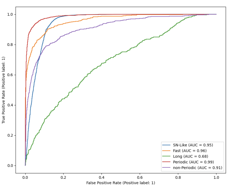
This study presents a bidirectional Long Short-Term Memory (LSTM) neural network for classifying transient astronomical object light curves from the Photometric LSST Astronomical Time-series Classification Challenge (PLAsTiCC) dataset. The original fourteen object classes were reorganized into five generalized categories (S-Like, Fast, Long, Periodic, and Non-Periodic) to address class imbalance. After preprocessing with padding, temporal rescaling, and flux normalization, a bidirectional LSTM network with masking layers was trained and evaluated on a test set of 19,920 objects. The model achieved strong performance for S-Like and Periodic classes, with ROC area under the curve (AUC) values of 0.95 and 0.99, and Precision-Recall AUC values of 0.98 and 0.89, respectively. However, performance was significantly lower for Fast and Long classes (ROC AUC of 0.68 for Long class), and the model exhibited difficulty distinguishing between Periodic and Non-Periodic objects. Evaluation on partial light curve data (5, 10, and 20 days from detection) revealed substantial performance degradation, with increased misclassification toward the S-Like class. These findings indicate that class imbalance and limited temporal information are primary limitations, suggesting that class balancing strategies and preprocessing techniques focusing on detection moments could improve performance.
📄 Full Content
Artificial intelligence (AI) has become increasingly important in scientific research, particularly for analyzing largescale datasets that exceed human processing capabilities. In astronomy, the exponential growth of observational data from modern telescopes requires automated classification systems to identify and categorize celestial objects efficiently. [1] Machine learning approaches, particularly deep neural networks, have shown great promise in handling such classification tasks.
Recently, the Large Synoptic Survey Telescope (LSST) proposed a challenge on Kaggle, a Google subsidiary website, Brazilian Centre for Physics Research 6th Edition of the Advanced School of Experimental Physics EAFExp called The Photometric LSST Astronomical Time-series Classification Challenge (PLAsTiCC). [2] This challenge is aimed at classifying light curves, data of the observed brightness of celestial objects as a function of time, which were simulated in preparation for LSST observations. These curves are capable of revealing the presence of some phenomena, such as supernovae [3]. The LSST will revolutionize our understanding of the sky, however, this type of study is hindered by the large volume of data obtained by the telescope, making automatic analysis procedures indispensable to differentiate and classify them. In this challenge, the question was raised: How well can we classify objects in the sky that vary in brightness from simulated LSST time-series data? The PLAsTiCC dataset and challenge were created to help classify these astronomical sources. [4] Before the use of AI, this type of classification still depended on manual analysis. Common statistical methods such as template fitting [5] were used, but these are not scalable for a large volume of data. Usually, a group of experts manually eliminated obvious cases of false positives, something that by itself can take several days. Of the remaining data, each case should be reviewed by at least three experts, which can lead to disagreements about a particular case, since experts might not have the same definition for classification. For these reasons, a reliable system is necessary that repeatedly selects the most important candidates that will be manually reviewed for confirmation at a later stage.
The light curve data were obtained through LSST PLAsTiCC via the Kaggle challenge [2]. To complete the project within the scheduled time of EAFEXP, a subset of the total data was used. In total, two datasets were used: the first had 7848 objects, of which 10% were used to form a validation set and the remainder formed the training set; the second dataset had 19920 objects and was used as the test set.
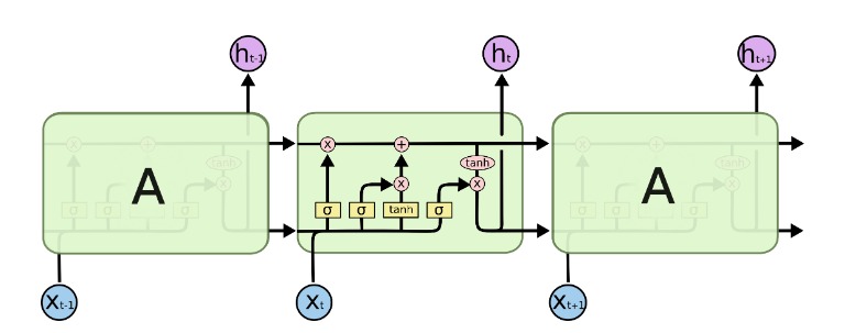
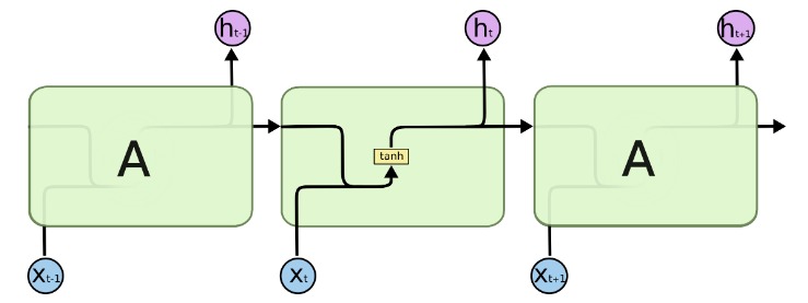
The data are in tabular format and consist of flux measurement information, measurement error, the measurement time Figure 2: Functioning of an LSTM network. [7] in Modified Julian Date (mjd), the filter used (the object’s emission spectrum, ugriZY, represented by a numerical value from zero to five), a boolean variable (0 or 1) that indicates detection or nondetection, the object class, and a unique identifier. An example can be seen in Table 1.
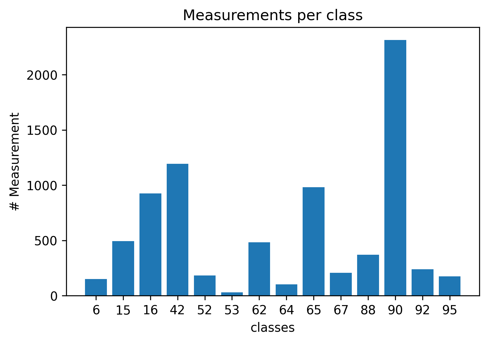
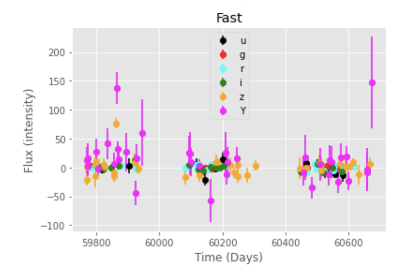
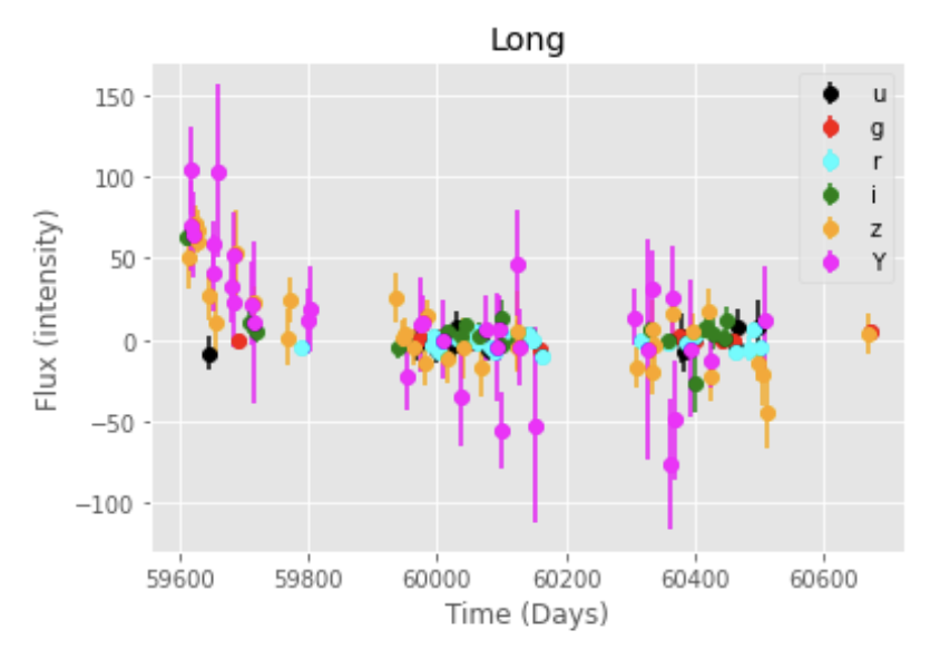
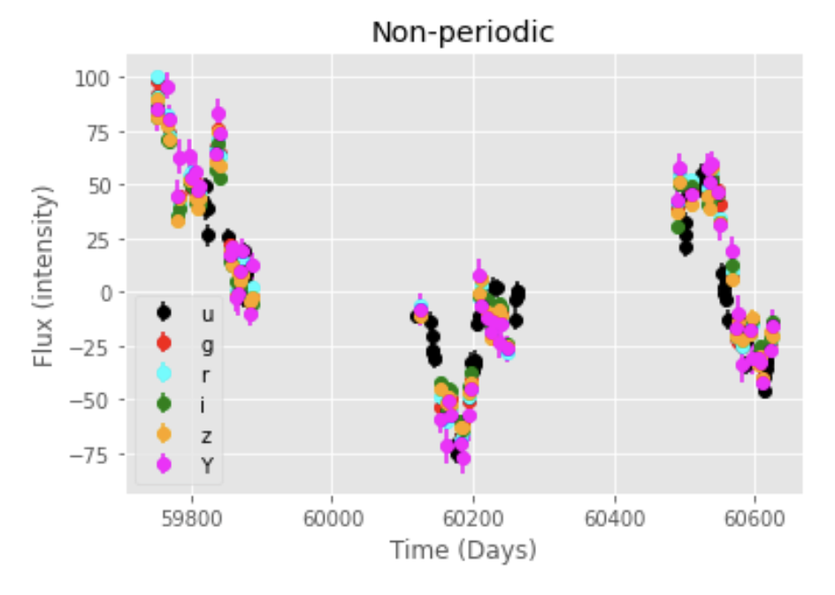
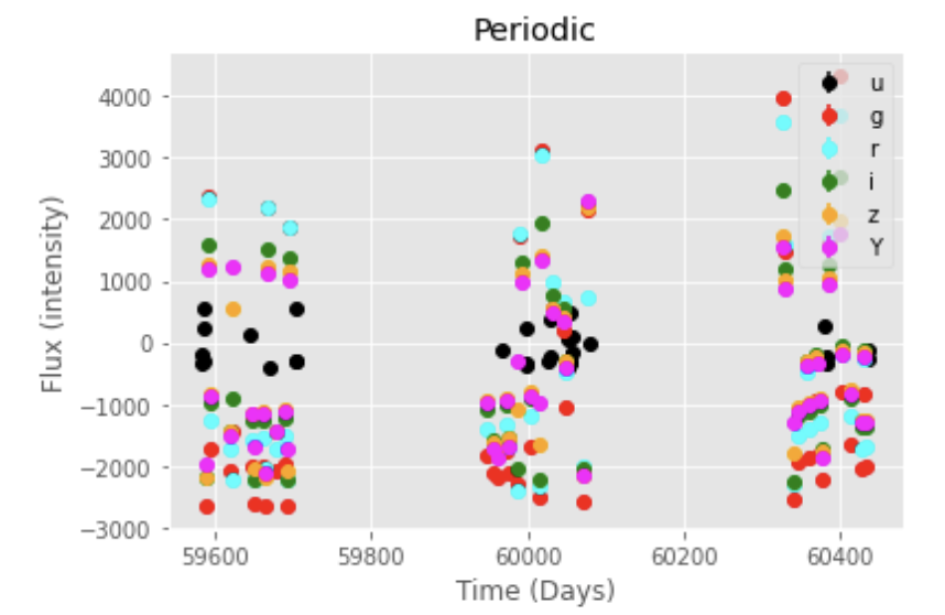
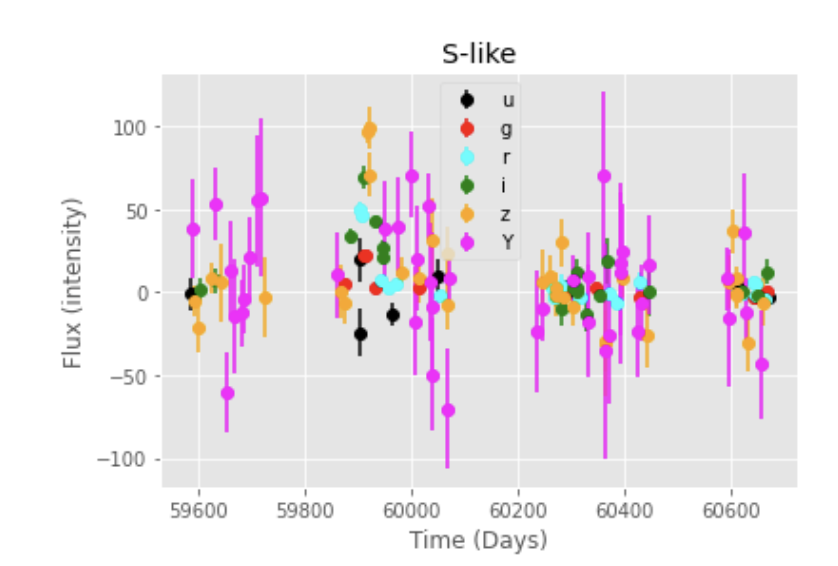
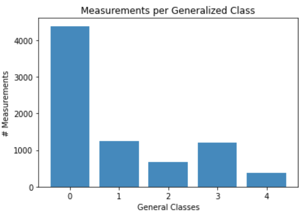
Initially, the provided data had fourteen categories, however, due to the discrepancy in the amount of data per category, the data were reorganized into five categories according to Table 2. Examples of each of the classes can be seen in figure 8. The distribution by original classes and generalized classes can be seen in figure 3.
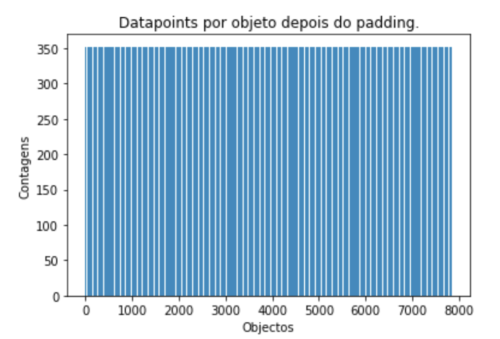
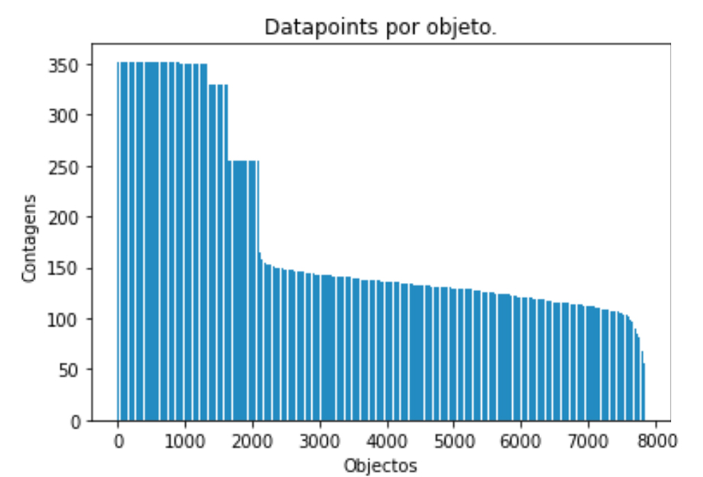
Id Original Class Generalized Class New Id Figure 3 To train the network, it is necessary to ensure that each object has the same number of measurements, since this will be the input dimension. This is not true for this dataset, so the data with smaller dimensions were filled with arbitrary values in a process known as padding. As shown in figure 4, after padding, all objects have the same dimension.
In addition, the temporal measurements were rescaled so that the first measurement of each object was set to zero on the temporal scale. Finally, the flux data were normalized for each object separately using min-max normalization, scaling values to the range [0,1], since the amplitude of measurements varies significantly between objects.
Finally, this project is interested in verifying the ability to classify objects with only partial light curve data. For this purpose, two new test sets were selected, where the data were advanced in time by ten and twenty days of observation from the moment each object is detected, and subsequently the network was evaluated with sets of five, ten, and twenty days into the future.
Since the provided data are time series, an LSTM network was chosen for its ability to capture temporal dependencies. The network is bidirectional to capture both forward and backward temporal patterns, as both previous and subsequent measurements are relevant for classification. Each column in the dataset (Table 1) was treated as a feature, resulting in five input features: flux, error, modified Julian date, filter, and detection.
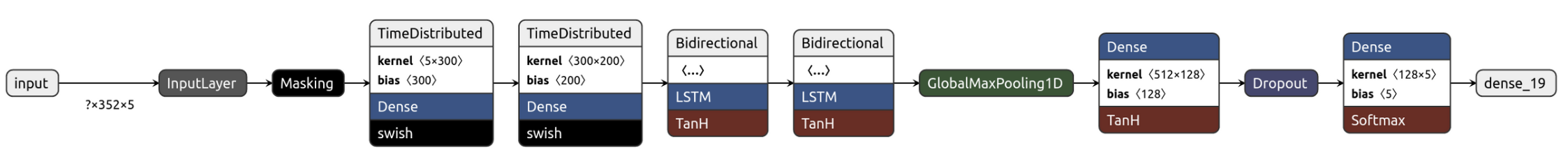
Due to the padding procedure, all objects have 352 measurements and 5 features. The network input dimensions are therefore 352×5, and the output is a probability distribution over the five generalized classes.
A masking layer was implemented to identify and ignore padded values, preventing them from being treated as noise. A GlobalMaxPooling layer was used to reduce the temporal dimensions by extracting the maximum value across the sequence, which helps capture the most significant features regardless of their temporal position. Finally, a dense layer with softmax activation performs the final classification. The complete network archi- Figure 4 tecture can be visualized in figure 5.
The network was trained using the Adam optimizer with categorical crossentropy as the loss function. Training was performed with early stopping based on validation loss to prevent overfitting. The model was trained for a maximum of 50 epochs with a batch size of 32.
All code used and the trained model to reproduce these results are available in a public repository on GitHub at the link https://github.com/MarcoBarroca/
VI_EAFEXP_Proj3.
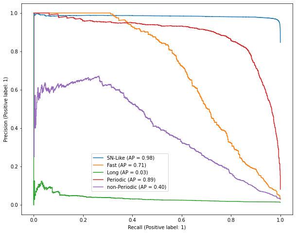
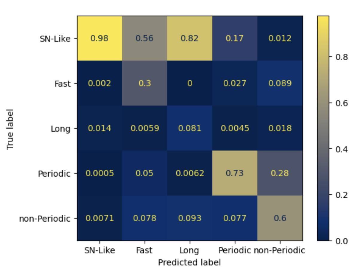
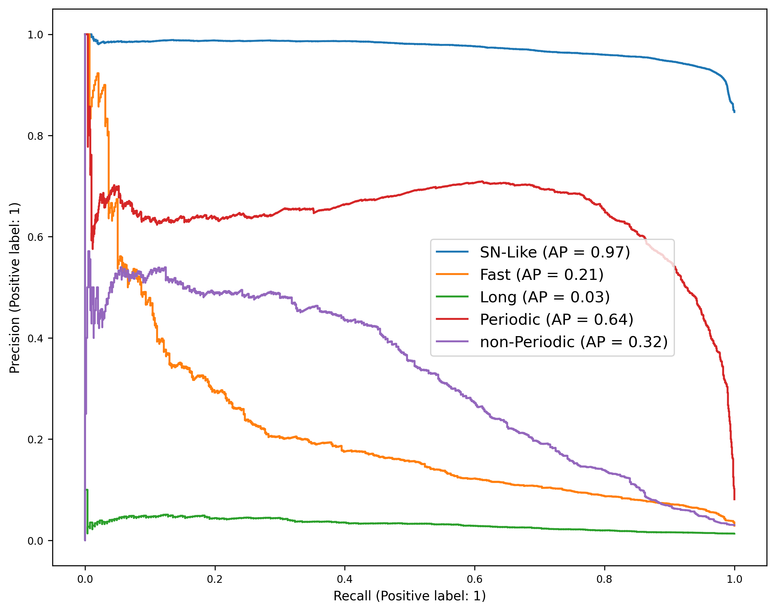
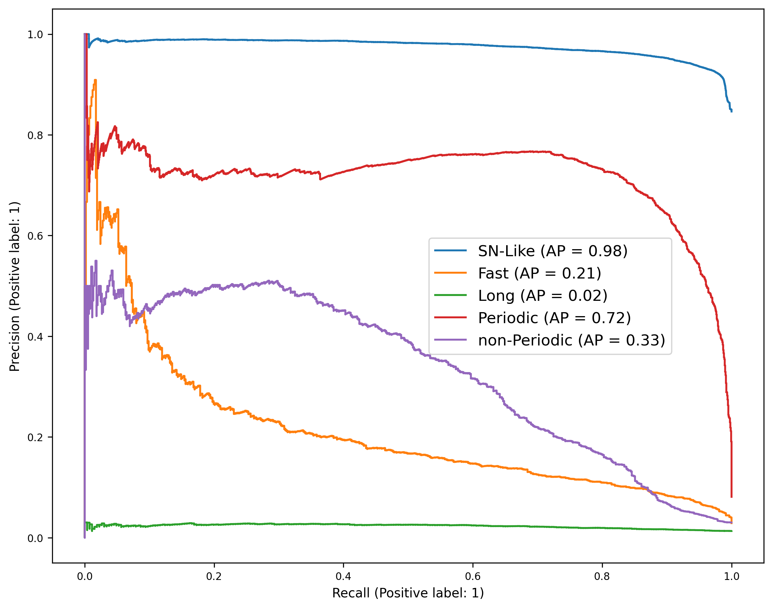
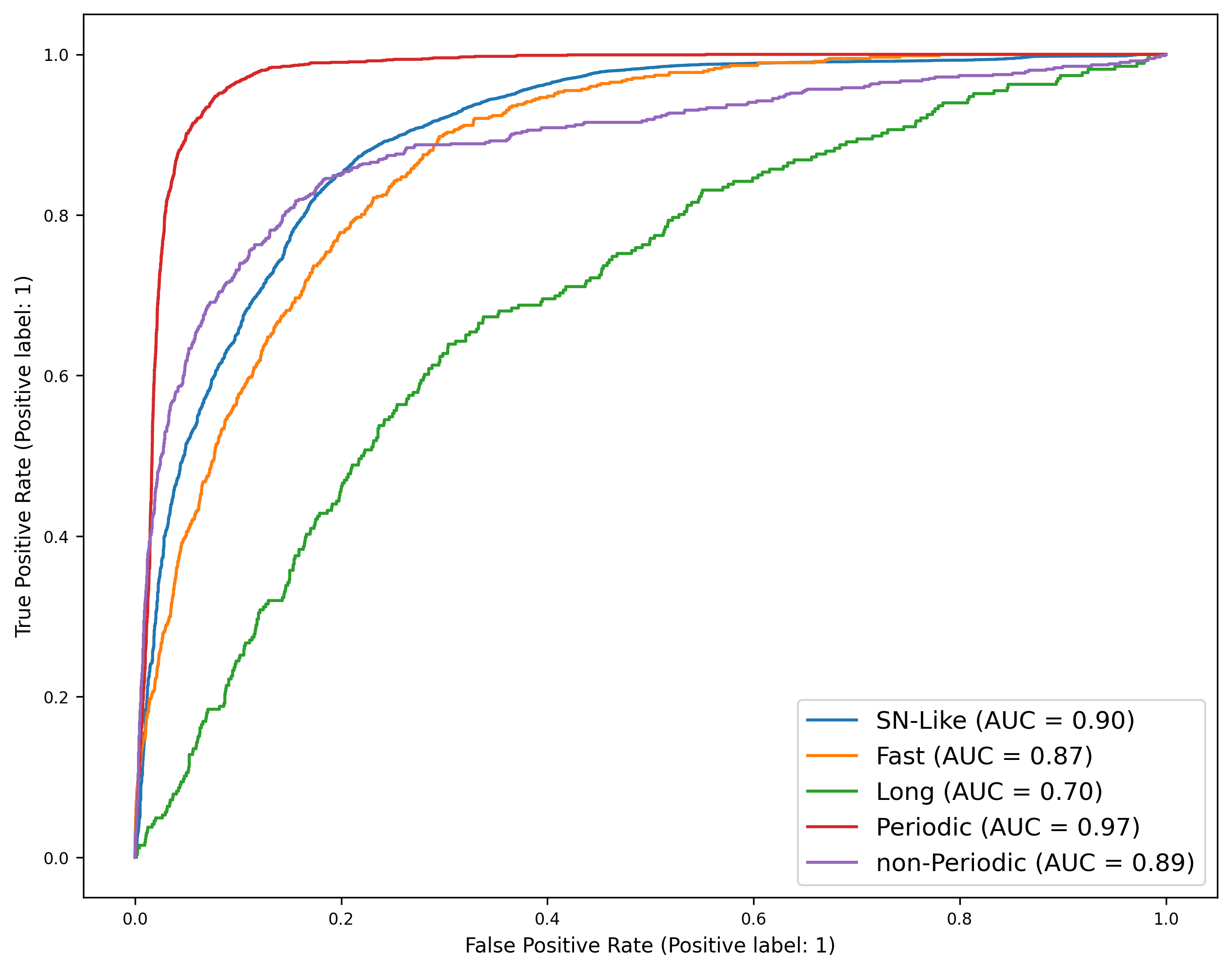
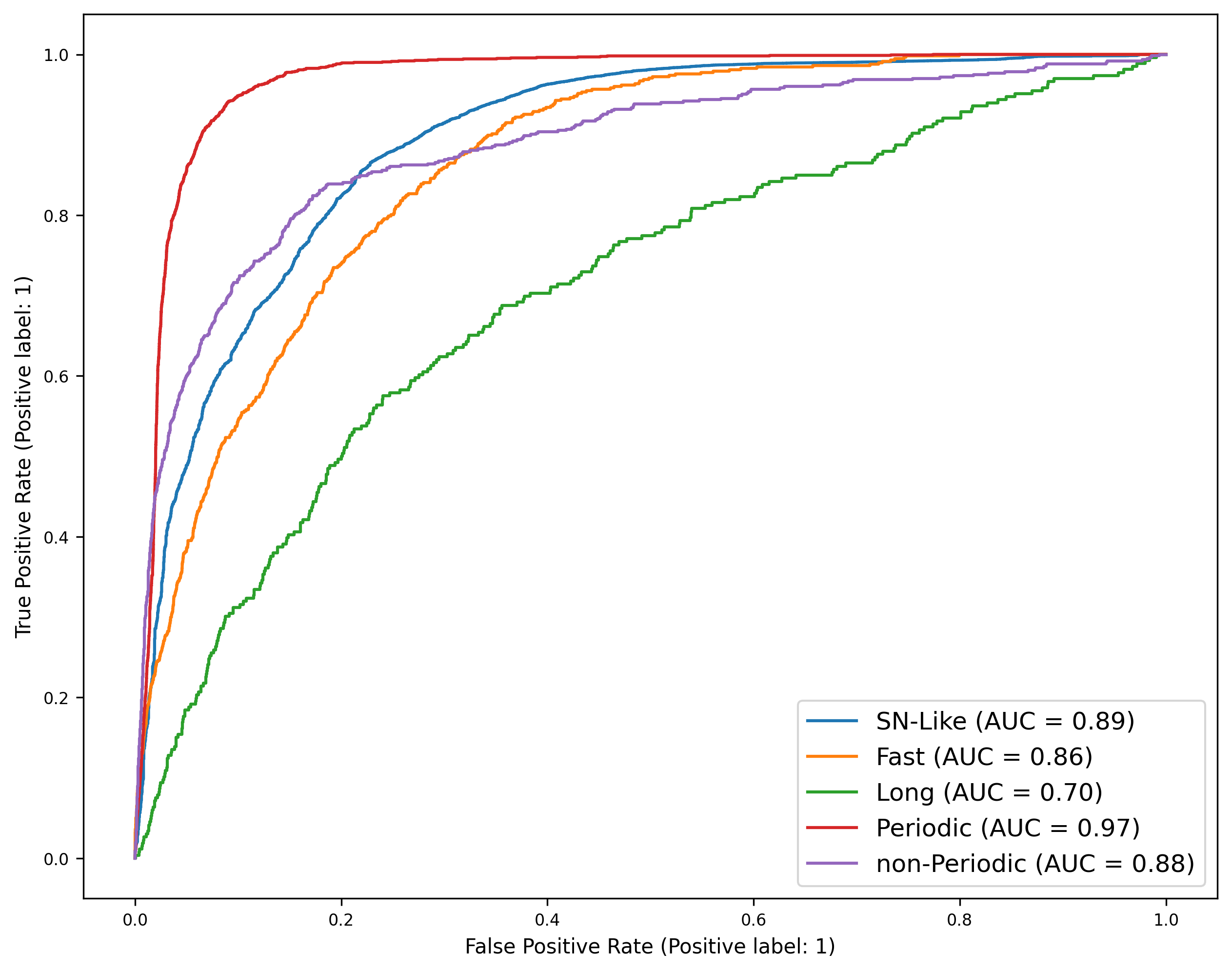
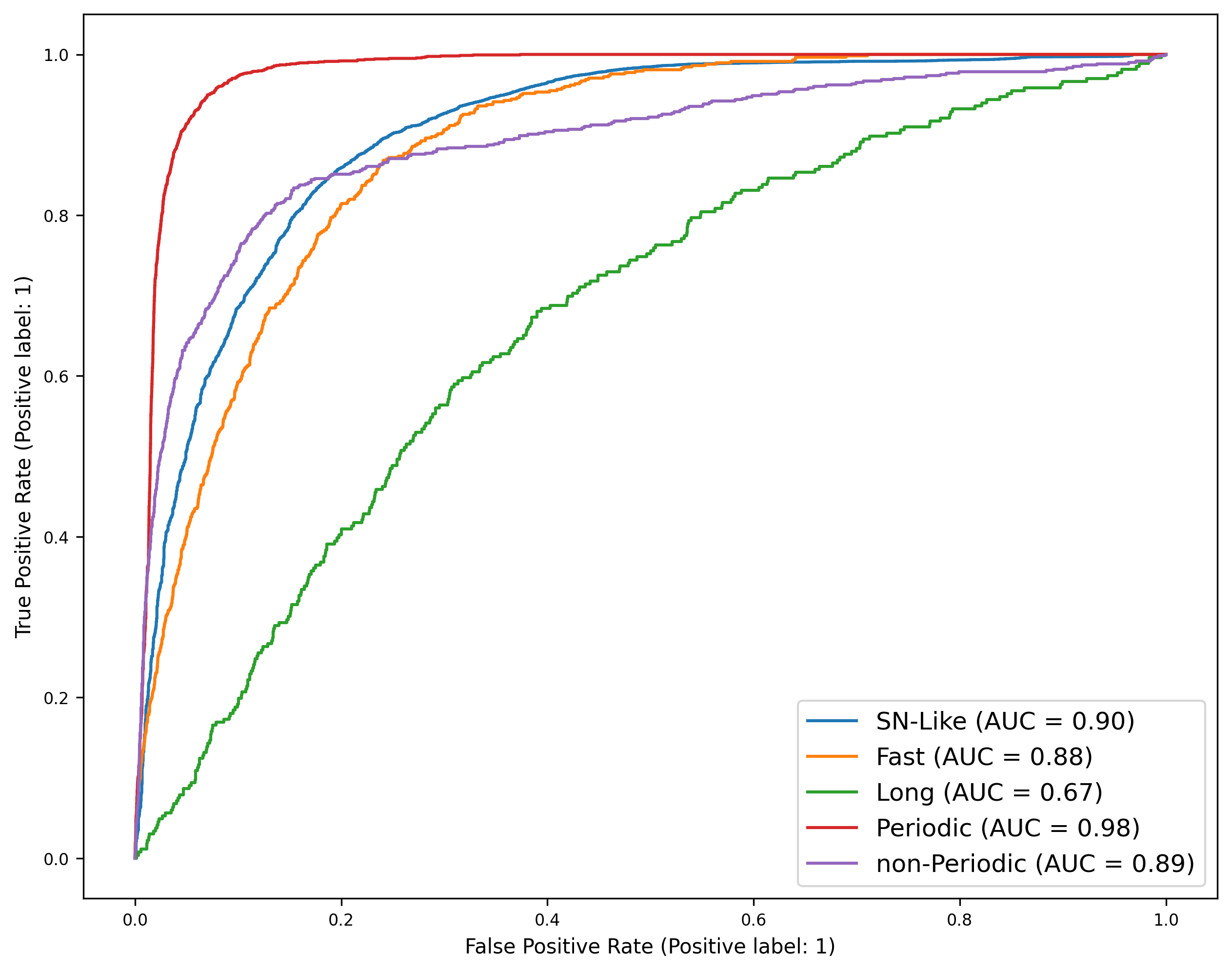
The network was evaluated using ROC curves, Precision-Recall curves, and confusion matrices, all constructed from the test set. The ROC curves showed excellent performance for the S-Like and Periodic classes, achieving area under the curve (AUC) values of 0.95 and 0.99, respectively. However, the Long class achieved a significantly lower AUC of 0.68, indicating poor performance for this
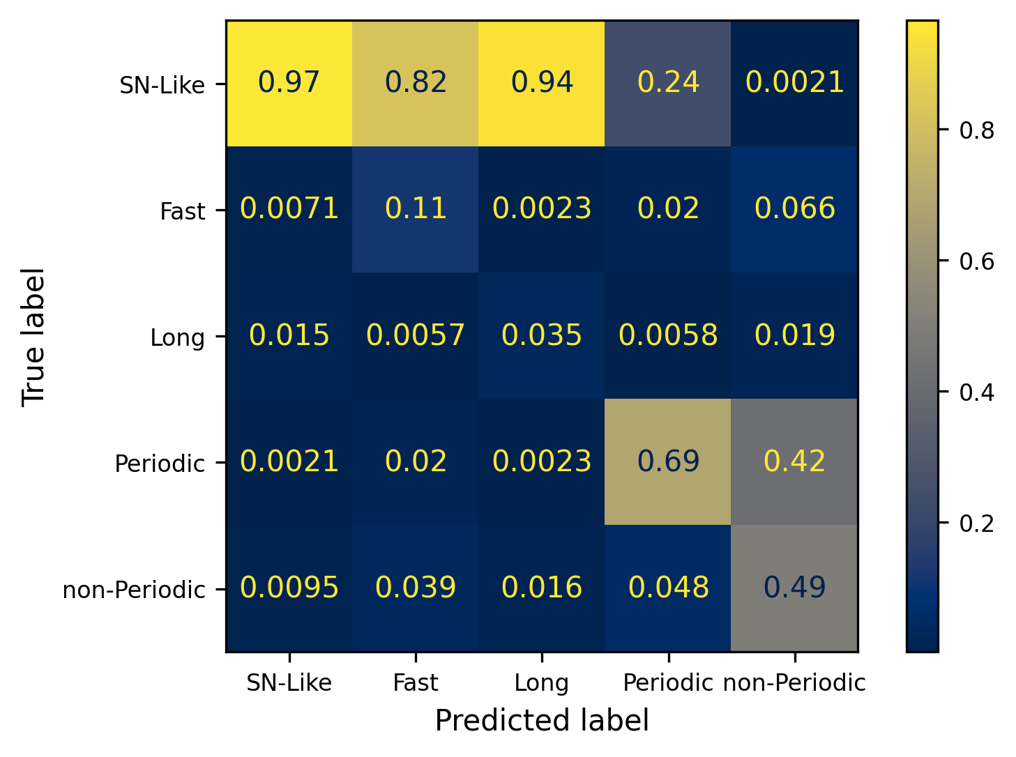
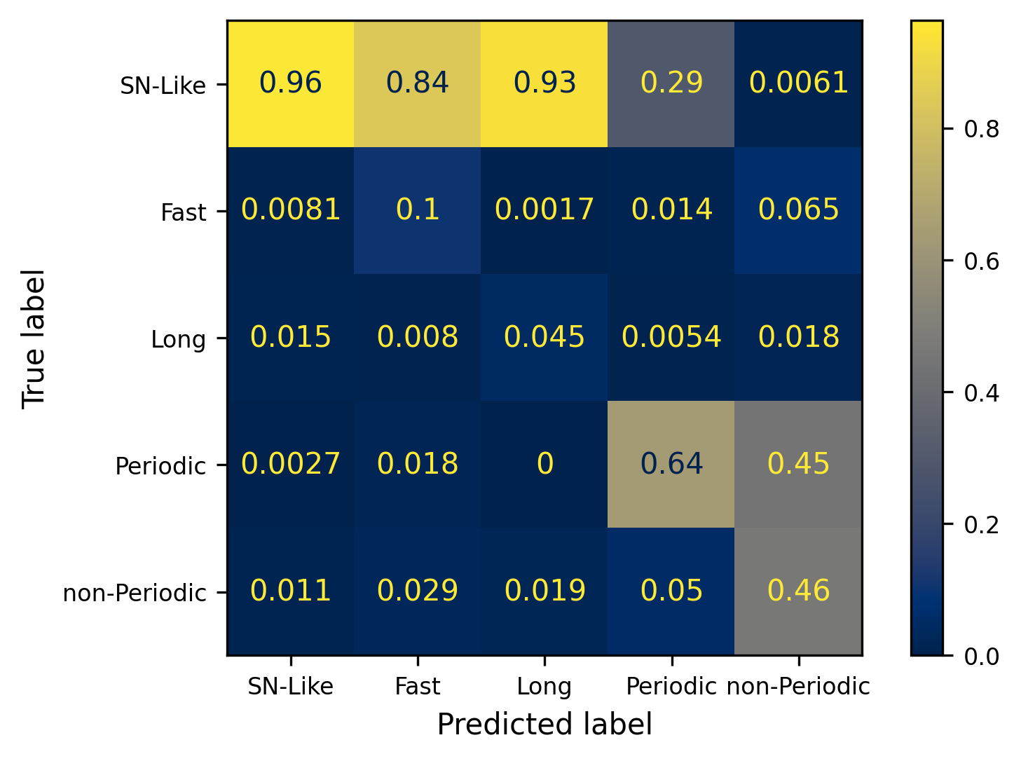
To assess the model’s ability to classify objects early in their light curve evolution, the network was evaluated on test sets with temporal advances of 5, 10, Figure 6 and 20 days from the detection moment. The results show a significant degradation in performance as the temporal advance increases. Even with only 5 days of advance, the network fails to achieve performance comparable to the complete dataset and begins to misclassify most objects as S-Like. This degradation becomes more pronounced with longer temporal advances, as shown in the confusion matrices in figure 7 (b), (c), and(d). The ROC and Precision-Recall curves for these partial datasets are provided in the Appendix (figures 9, 10, and 11).
This work presents a bidirectional LSTM neural network for classifying transient astronomical object light curves from the PLAsTiCC dataset. The model achieved strong performance for S-Like and Periodic classes, with ROC AUC values of 0.95 and 0.99, respectively, demonstrating the effectiveness of LSTM networks for time-series classification in astronomy.
However, several limitations were identified. The model struggled significantly with Fast and Long classes, likely due to their characteristic short-duration peaks that occur only at the beginning or end of measurements, making them difficult to capture with the current ap- Several approaches could address these limitations. First, class balancing through oversampling underrepresented classes or using more sophisticated class weighting schemes could improve performance on minority classes. Second, preprocessing strategies that focus on detection moments (using only data where the detection variable equals 1) could help capture the characteristic features of Fast
Brazilian Centre for Physics Research 6th Edition of the Advanced School of Experimental Physics