The Complexity of Contracting Planar Tensor Network

Algorithms for contracting tensor networks
Kourtis et al. introduced an algorithm to contract a planar Boolean tensor network in $`2^{O(\sqrt{\Delta}N)}`$ time, where $`N`$ denotes the number of vertices and $`\Delta`$ denotes the maximum degree. They presented a divide and conquer algorithm to find a sequence of edge separators to partition the network to $`N`$ isolated tensors, according to Lemma [planar_edge_separator]. Then they contracted the isolated tensors in the reversed order of partitioning. The algorithm guaranteed that each tensor appearing in the contraction process has $`O(\sqrt{\Delta N})`$ dimension so that the Boolean tensor network can be contracted in $`2^{O(\sqrt{\Delta N})}`$ time.
Inspired by the algorithm, we consider the edge separator of a finite element graph.
Let $`G`$ be a finite element graph with $`N`$ vertices and maximum degree $`\Delta`$. Suppose each element of $`G`$ has no more than $`d`$ boundary edges. A balanced edge separator $`C`$ of $`G`$ can be found in polynomial time, with $`|C|=O(d\sqrt{\max\{\Delta,d\}N})`$.
Proof. Let $`G^*`$ denotes the planar skeleton of $`G`$. Suppose $`G^*`$ has $`f`$ faces $`L_1,L_2,...,L_f`$ with more than $`3`$ boundary edges. We construct a planar graph $`G^{**}`$ from $`G^{*}`$ by adding a new vertex $`w_i`$ inside each face $`L_i`$ and connecting it with all boundary vertices. $`W=\{w_1,w_2,...,w_f\}`$. The planar graph $`G^{**}`$ has $`N+f\leq 2N`$ vertices and maximum degree $`\Delta^{**}\leq \mathrm{max}\{\Delta,d\}`$. By Lemma [separator_for_finite_element_graph], we find a balanced edge separator $`C^{**}`$ with $`|C^{**}|=O(\sqrt{\Delta^{**}N})`$ in $`O(N)`$ time.
Suppose $`C^{**}`$ partitions $`G^{**}`$ into two disconnected parts $`A^{**}`$ and $`B^{**}`$. Let $`A=A^{**}\cap V(G)`$ and $`B=B^{**}\cap V(G)`$. For an edge $`(u,v)\in E(G)`$ which connects $`A`$ and $`B`$, either $`(u,v)\in C^{**}`$ or $`\{(u,w_i),(w_i,v)\}\cap C^{**}\neq\emptyset`$ for some $`w_i\in W`$. If $`(u,w_i)\in C^{**}`$, we add all diagonals, which connect $`u`$ with some boundary vertex of $`L_i`$, to the set $`C`$. We do the same if $`(w_i,v)\in C^{**}`$. Finally, we add $`C^{**}\cap E(G)`$ to $`C`$. $`C`$ is a balanced edge separator of $`G`$ and $`|C|=O(d\sqrt{\max\{\Delta,d\}N})`$. ◻
Then we can build an exponential algorithm similar to the algorithm in .
Let $`G`$ be a finite element with $`N`$ vertices and maximum degree $`\Delta`$. Suppose each element of $`G`$ has no more than $`d`$ boundary edges. Given a Boolean tensor network whose underlying graph is $`G`$, it can be contracted in $`2^{O(d\sqrt{\max\{\Delta,d\}N})}`$ time.
Defined on a set of Boolean symmetric functions
We consider accelerating the above algorithms. When the tensor network is defined on a set of Boolean symmetric functions, we replace each function of some arity $`n`$ by a planar bounded degree gadget with $`O(n)`$ vertices.
Suppose $`F=[f_0,f_1,\cdots,f_n]`$ with $`f_0,f_1,...,f_n\in\mathbb{C}`$ (w.l.o.g, $`n`$ is a power of $`2`$)1. We replace $`F`$ with an equivalent planar gadget, shown in Figure 1. The general idea of the gadget is to rearrange the assignment of variables since the order of elements in the assignment is irrelevant. Treating each assignment as an $`n`$-length string over $`\{0,1\}`$, we use the left part to count the number of $`1`$ (Hamming weight) and use the right part to return an ordered $`n`$-length string where all $`1`$ are in front of $`0`$. Then we decide the corresponding function value according to the location of the border of $`1`$ and $`0`$. Next, we introduce the gadget in detail.
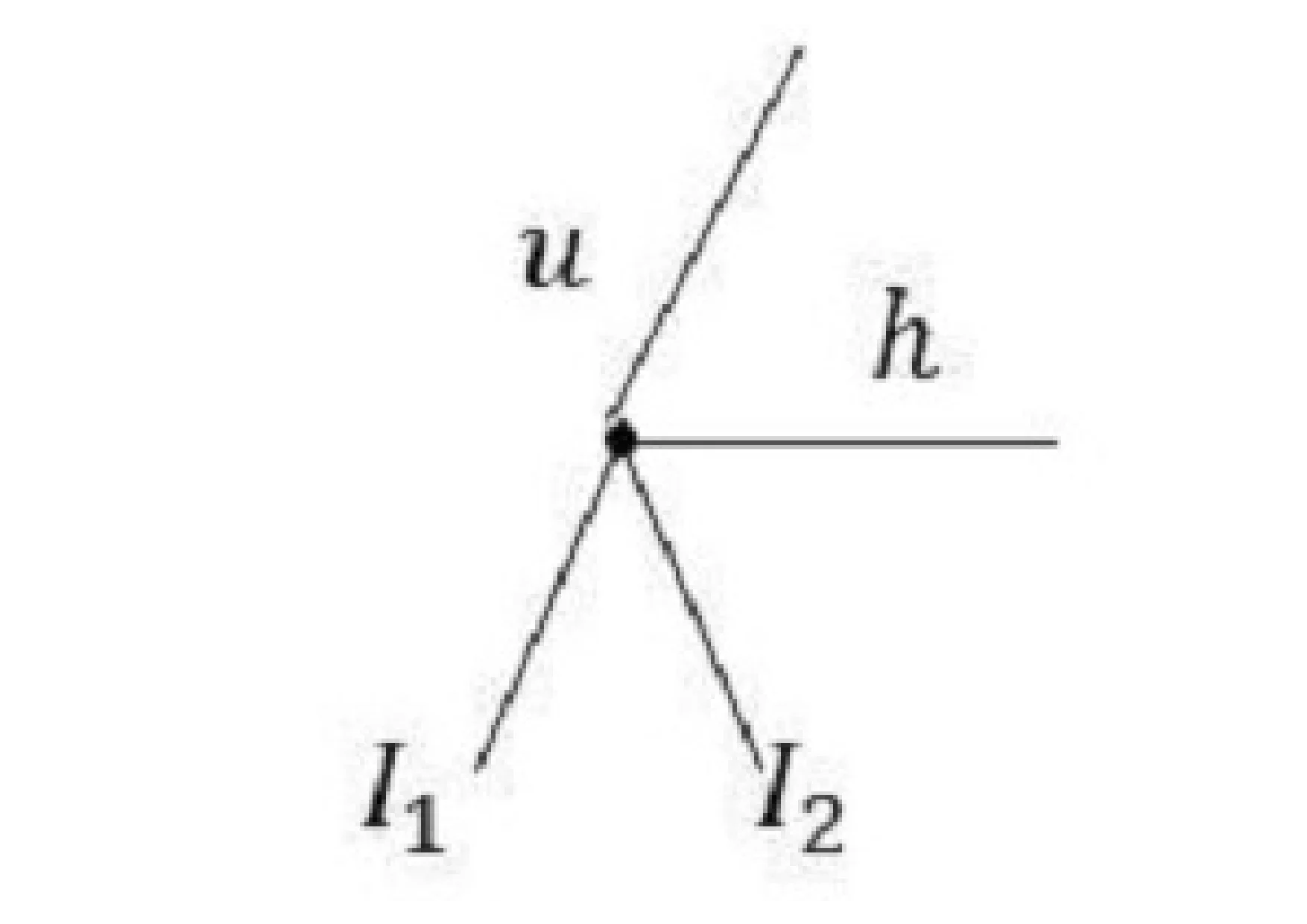
The left part of this planar gadget uses the idea “Adder” to calculate the binary expression of Hamming weight $`Hw(x)`$ of the assignment $`x=(w_1w_2\cdots w_n)\in\{0,1\}^n`$. The functions all are simple addition operators in the left part. The left structure accepts $`x`$ and adds every two adjacent bits. Each vertex denotes an addition function $`A`$ or $`B`$, shown in Figure 2-(a), which adds two bits $`I_1, I_2`$ or three bits $`h_1, I_1, I_2`$, sets the most significant bit $`u`$ to join a higher level addition, and sets the least significant bit $`h`$ or $`h_2`$ to join the operation of the horizontal adjacent vertex on the right. After $`\log_2 n`$ levels, the left part outputs the binary expression of $`{\rm Hw}(x)`$ in the horizontal edges from top to bottom (information would not be lost since $`{Hw}(x)\leq \log_2 n +1`$).


\begin{align*}
        &A(u,h,I_1,I_2)=
        \begin{cases}
            1  &  \text{if $u=\lfloor (I_1 + I_2)/2 \rfloor $ and $h=(I_1+I_2)$ mod 2} \\
            0 &  \text{else}\\
        \end{cases}
        \\
        &B(u,h_1,h_2,I_1,I_2)=
        \begin{cases}
            1  &  \text{if  $u=\lfloor(I_1 + I_2 + h_1)/2\rfloor$ and $h_2=(I_1+I_2+h_1)$ mod 2} \\
            0 &  \text{else}\\
        \end{cases}
\end{align*}
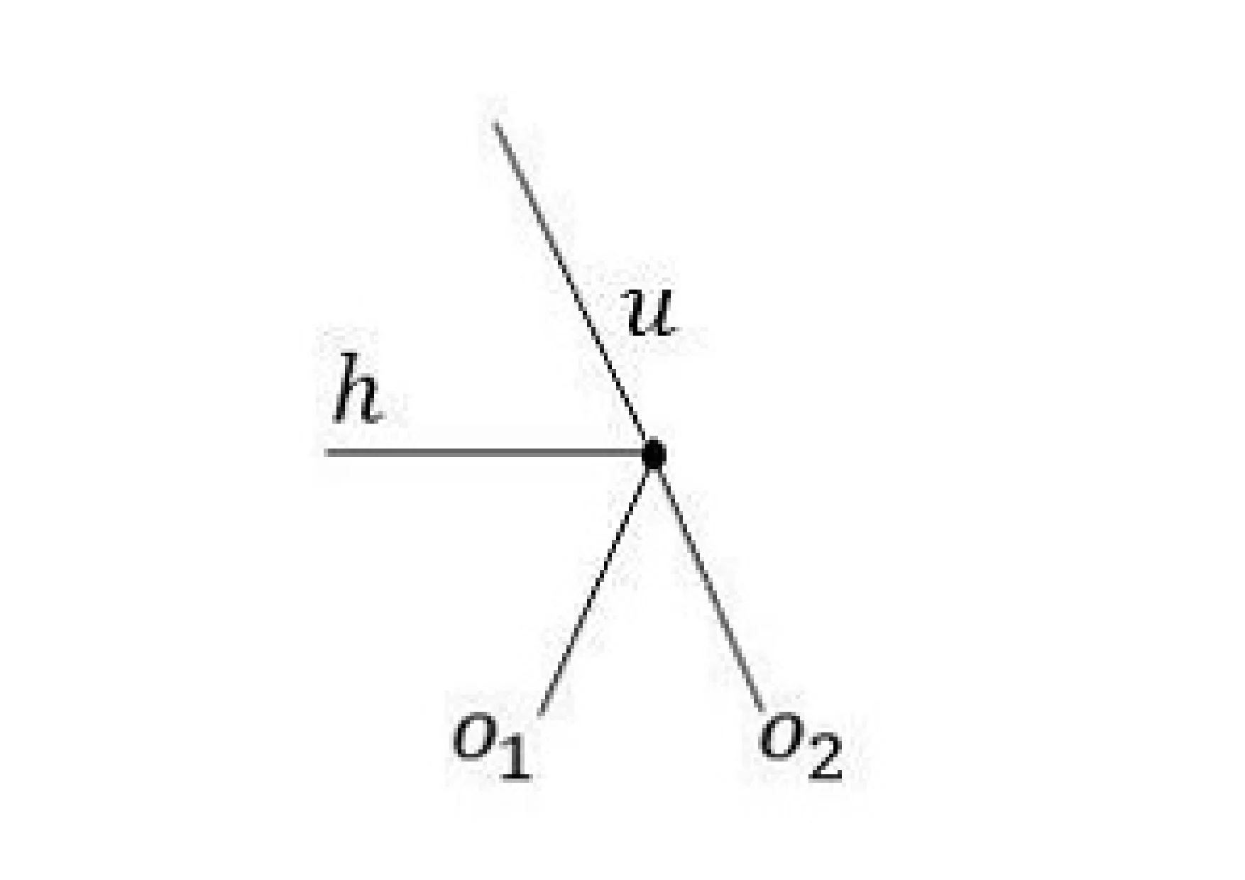
The right part uses the horizontal $`(\log_2 n+1)`$ bits to recover an ordered string of the form $`1^{{\rm Hw}(x)} 0^{|x|-{\rm Hw}(x)}`$ before outputting the accuracy value of $`F`$. It is obvious that the top two bits would not be $`1`$ at the same time. In the right part, the functions are a little different from those in the left part, shown in Figure 2-(b). Each of them is one of the following functions:
\begin{align*}
        &C(u,h,o_1,o_2)=
        \begin{cases}
            1 &  \text{if $o_1=u + h$ and $o_2= 2u+h-o_1$} \\
            0 &  \text{else}\\
        \end{cases}
        \\
        &D(u,h_1,h_2,o_1,o_2)=
        \begin{cases}
            1 &  \text{if $u=1$ \& $o_1=o_2=1$ and $h_2=h_1$} \\
            1 &  \text{if $u=0$ \& $o_1=h_1$ and $o_2=h_2=0$} \\
            0 &  \text{else}\\
        \end{cases}
\end{align*}
The Hamming weight is reflected by the location of the sub-string $`10`$ in the ordered string $`1^{{\rm Hw}(x)} 0^{|x|-{\rm Hw}(x)}`$. The gadget uses additional $`2`$-arity functions $`F_1,\cdots,F_i,\cdots,F_{n-1}`$ to identify the location, where $`i\in \{2,\cdots,n-2\}`$.
\begin{equation}
    \begin{cases}
    F_1(0, 0)=f_0, &   \\
    F_1(1, 0)=f_1, &  \\
    F_1(1, 1)=F_1(0,1)=1; &
    \end{cases}
    \nonumber
\end{equation}
\begin{align*}
        &\begin{cases}
            F_i(0,0)=F_i(1,1)=F_i(0,1)=1, &   \\
            F_i(1,0)=f_i; &
        \end{cases}
    \\
        &\begin{cases}
            F_{n-1}(1,1)=f_n, &   \\
            F_{n-1}(1,0)=f_{n-1}, &  \\
            F_{n-1}(0,0)=F_{n-1}(0,1)=1. &
        \end{cases}
\end{align*}
The number of vertices in such a planar gadget is $`2(n+ \frac{n}{2} + \frac{n}{4} + \cdots +1 ) + n-1 = O(n)`$, and the maximum degree is $`5`$.
For any tensor network $`G`$ defined on the set of Boolean symmetric functions, we preprocess it to a bounded degree tensor network $`G'`$ by the above gadgets. If $`G`$ is planar, then $`\sum_{v\in V(G)} d_{v}=2E(G)\leq 6|V(G)|-12`$. So $`G'`$ has $`O(|V(G)|)`$ vertices. We apply the algorithm on $`G'`$.
Any planar tensor network consisting of $`N`$ Boolean symmetric tensors can be contracted in $`2^{O(\sqrt{N})}`$ time.
If $`G`$ is a finite element graph, we need more steps to preprocess $`G`$. We transfer $`G`$ to a planar graph first. Suppose there are $`f`$ elements $`L_1,L_2,...,L_f`$ with more than $`3`$ boundary edges in the planar skeleton $`G^*`$ of $`G`$. $`d_i`$ denotes the number of boundary edges in $`L_i`$ for $`i\in[f]`$. There are no more than $`(\sum_{i\in [f]} d_i^4)`$ crossings in $`G`$, according to the definition of finite element graphs. We replace each crossing with a new vertex assigned with the function $`Cr`$, shown in Figure 3. The function $`Cr`$ keeps $`a=a'`$ and $`b=b'`$ for Boolean variables $`a,a',b,b'`$.

Then we obtain a planar tensor network $`G'`$with no more than $`N+\sum_{i\in [f]} d_i^4\leq N+2m d^3\leq N+ 6Nd^3`$ vertices, where $`m=|E(G^*)|\leq |E(G)|`$ and $`d=\mathrm{max}\{d_1,...,d_f\}`$. $`Z(G')=Z(G)`$. A gadget with the function $`Cr`$, shown in Figure 3, consists of only Boolean symmetric functions. We construct the planar $`G''`$ from $`G'`$ by replacing each occurrence of $`Cr`$ with such a gadget. $`G''`$ has $`O(d^3N)`$ vertices and maximum degree no more than $`6`$. $`Z(G'')=Z(G')=Z(G)`$. We can compute $`Z(G'')`$ in $`2^{O(\sqrt{d^3N})}`$ time by Theorem [thm4]. Since $`G''`$ is constructed in polynomial time, the above algorithm computes $`Z(G)`$ in $`2^{O(\sqrt{d^3N})}`$ time.
A tensor network consisting of $`N`$ Boolean symmetric tensors can be contracted in $`2^{O(\sqrt{d^3N})}`$ time if the underlying graph is a finite element graph whose elements all have no more than $`d`$ boundary edges.
Can we also construct a planar bounded degree gadget for any symmetric function over a larger domain, for example, the domain $`[3]`$? The algorithm in Theorem [thm3] can be extended further if we can. Unfortunately, the answer is negative, according to Appendix A.
Defined on a set of finite functions
It is trivial that a tensor network consisting of only unary functions can be contracted in polynomial time. $`CP`$ decomposition provides the way to decompose a tensor to a series of unary functions.
Let $`\mathcal{F}`$ be a finite set of functions and $`R=\mathrm{max}\{rank(F)|F\in\mathcal{F}\}`$. A planar tensor network defined on $`\mathcal{F}`$ can be contracted in $`R^{O(\sqrt{N})}`$ time, where $`N`$ denotes the number of vertices in the input.
Proof. We state the main idea of the divide and conquer algorithm here. Appendix A.1 shows details.
Given a planar tensor network $`G`$ with $`N`$ vertices, we search for a balanced node separator $`C`$ with $`|C|=O(\sqrt{N})`$ in linear time, by Lemma [planar_node_separator]. For each vertex $`v\in C`$, we replace the $`d_v`$-dimensional tensor $`F_v`$ by the components of a minimum $`CP`$ decomposition of $`F_v`$ independently. Suppose $`F_v=\sum_{i=1}^{r} u_{i}^{1}\otimes u_{i}^{2}\otimes \dots \otimes u_{i}^{d_v}`$, where $`r=rank(F_v)\leq R`$, then we obtain a series of new tensor networks $`G_1,...,G_r`$ by replacing $`F_v`$ with $`r`$ components $`u_{1}^{1}\otimes u_{1}^{2}\otimes \dots \otimes u_{1}^{d_v},...,u_{r}^{1}\otimes u_{r}^{2}\otimes \dots \otimes u_{r}^{d_v}`$ independently. We make a contraction between each $`u_{i}^{j}`$ and its adjacent tensor in $`G_i`$, where $`j\in[k]`$. After the contractions, $`G_i`$ is a tensor network consisting of two disconnected planar tensor networks $`A_i`$ and $`B_i`$, where each has no more than $`\frac{2}{3}N`$ vertices. Suppose $`Z(G)`$ denotes the value of $`G`$. $`Z(G)=\sum_{i=1}^{r} Z(G_i)=\sum_{i=1}^{r} Z(A_i)Z(B_i)`$. Then we compute $`Z(A_i)`$ and $`Z(B_i)`$ for $`i\in[r]`$.
The value of $`G`$ can be computed in $`R^{O(\sqrt{N})}`$ time by the above algorithm. The runtime analysis is presented in Appendix B. ◻
The above algorithm can be extended for contracting tensor networks on finite element graphs, by Lemma [separator_for_finite_element_graph].
Let $`\mathcal{F}`$ be a finite set of functions and $`R=\mathrm{max}\{rank(F)|F\in\mathcal{F}\}`$. A tensor network defined by $`\mathcal{F}`$, whose underlying graph is a finite element graph having no elements with more than $`d`$ boundary edges, can be contracted in $`R^{O(d\sqrt{N})}`$ time, where $`N`$ is the number of tensors.
Lower bounds of tensor network contraction problems
In this section, we prove the lower bound for contracting tensor networks, even restricting the underlying graphs to planar graphs or finite element graphs.
If #ETH holds, then there is a constant $`\varepsilon>0`$ such that a planar tensor network can not be contracted in $`2^{\varepsilon \sqrt{N}}`$ time, where $`N`$ denotes the number of vertices in the input.
Furthermore, the result holds for the planar tensor networks defined by the set $`\{=_2,=_3,\neq_2,OR_3\}`$.
Proof. We reduce the problem #$`\{=_2,=_3,\neq_2,OR_3\}`$ to $`pl`$-#$`\{=_2,=_3,\neq_2,OR_3\}`$. Let $`G`$ with $`N`$ vertices be an instance of #$`\{=_2,=_3,\neq_2,OR_3\}`$. $`G`$ has at most $`3N`$ edges and $`9N^2`$ crossings.
We replace each crossing with a new vertex assigned the function $`Cr`$. The new tensor network $`G'`$ is an instance of $`pl-\#\{=_2,=_3,\neq_2,OR_3,Cr\}`$. $`G'`$ has at most $`(N+9N^2)`$ vertices. We replace each occurrence of $`Cr`$ with the gadget shown in Figure 3, then we construct a planar tensor network $`G''`$with $`O(N^2)`$ vertices. $`G''`$ is an instance of $`pl`$-#$`\{=_2,=_3,\neq_2,OR_3,OR_2,=_5,=_6\}`$. We further replace each occurrence of $`OR_2`$, $`=_5`$, or $`=_6`$ by the gadgets shown in Figure 4. The generated tensor network $`G'''`$ is an instance of $`pl`$-$`\#\{=_2,=_3,\neq_2,OR_3\}`$. $`G'''`$ has $`O(N^2)`$ vertices. $`Z(G''')=Z(G'')=Z(G')=Z(G)`$.


Suppose the theorem is false, i.e., we can solve $`Z(G''')`$ in $`2^{\varepsilon \sqrt{cN^2}}`$ time for any $`\varepsilon>0`$, then we can solve $`Z(G)`$ in $`\mathrm{poly}(N)+2^{\varepsilon \sqrt{cN^2}}\leq2^{\varepsilon'N}`$ time for some constant $`\varepsilon'`$. It is a contradiction to Lemma [lower_bound_of_3SAT]. ◻
Now we think about the lower bound for tensor network contraction problems on finite element graphs. Given a planar graph, we use triangular partitioning to build a finite element graph.
If #ETH holds, then there is a constant $`\varepsilon>0`$ such that a tensor network, whose underlying graph is a finite element graph with $`N`$ vertices, can not be contracted in $`2^{\varepsilon \sqrt{N}}`$ time.
Furthermore, the result holds even when the parameterized set is restricted to Boolean symmetric functions of arity no more than $`7`$.
Proof. Let $`G`$ be an instance of $`pl-\#\{=_2, =_3, \neq_2, OR_3\}`$. The underlying graph has a planar embedding, which $`G`$ also denotes. For the embedded planar graph $`G`$, we think about triangular partitioning every face with more than $`3`$ boundary edges. We first deal with bridges. We add a new vertex $`w`$ and edges $`(v_1,w),(v_2,w)`$ for each bridge $`(v_1,v_2)`$. Then we get a new planar graph $`G'`$ with no bridge. Let $`L_1,L_2,...,L_s`$ denote the faces with more than $`3`$ boundary edges in $`G'`$.
Suppose the boundary vertices of a face $`L\in\{L_1,L_2,...,L_s\}`$ are labeled $`v_1,v_2,...,v_{d}`$ in clockwise order 2. We add a $`(\lceil \frac{d}{2}\rceil)`$-length cycle $`(u_1,u_2,...,u_{\lceil d/2 \rceil },u_1)`$ inside $`L`$, and add edges $`(u_j,v_{2j-1}),(u_j,v_{2j}),(u_j,v_{2j+1})`$ for $`j\in\{1,2,..,\lfloor d/2 \rfloor\}`$, where $`v_{d+1}`$ is exact $`v_1`$. If $`d`$ is odd, we extra add the edges $`(u_{\lceil d/2 \rceil},v_{d})`$ and $`(u_{\lceil d/2 \rceil},v_{d_1})`$. We partition $`L`$ into some triangles and a face $`L'`$ with $`(\lceil d/2 \rceil )`$ boundary edges. We continue to partition $`L'`$ in the same way. After no more than $`\lceil log_2 d \rceil`$ rounds, we completely triangulate $`L`$. We add no more than $`d`$ new vertices with degree no more than $`7`$. For example, we show in Figure 5 the process of partitioning a face with $`7`$ boundary edges.

We triangulate each face in $`G'`$ and obtain a finite element graph $`G''`$ in $`\mathrm{poly}(N)`$ time. The planar skeleton of $`G''`$ is itself. $`G''`$ has no more than $`N+\sum_{L_i} d_i\leq N+2|E(G')|\leq6N`$ vertices, where $`d_i`$ is the number of boundary edges in face $`L_i`$. The maximum degree of $`G''`$ is no more than $`7`$.
Next, we assign to every vertex $`v\in V(G'')`$ an appropriate Boolean symmetric function, such that $`Z(G')=Z(G)`$. For each vertex $`v\in V(G'') - V(G)`$, we assign the function $`[1,0]^{\otimes d_v}`$ to $`v`$, so that the edge-variables in $`E(G'')-E(G)`$ must be assigned $`0`$. For each vertex $`v\in V(G'')\cap V(G)`$, we assign to $`v`$ the function $`F_v`$, according to the function $`[f_0,f_1,f_2,f_3]`$ (or $`[f_0,f_1,f_2]`$) which is originally assigned to $`v`$ in $`G`$. $`F_v`$ denotes the function $`[0,...,0,f_0,f_1,f_2,f_3]`$ (or function $`[0,...,0,f_0,f_1,f_2]`$), which takes value $`0`$ when the Hamming weight of input is no more than $`k-4`$ (or $`k-3`$). The assignment to edges in $`E(G'')-E(G)`$ are fixed and make no difference to the value of $`G''`$. The assignments to edges $`E(G’')\cup E(G)`$ contribute to $`Z(G'')`$ in the same way as they contribute to $`Z(G)`$. So $`Z(G‘')=Z(G)`$.
Suppose $`Z(G'')`$ can be solved in $`2^{\varepsilon\sqrt{6N}}`$ time for any $`\varepsilon>0`$, then we have an algorithm to compute $`Z(G)`$ in $`(\mathrm{poly}(N)+2^{\varepsilon\sqrt{6N}})\leq2^{\varepsilon’ \sqrt{N}}`$ time for some $`\varepsilon'>0`$. It is a contradiction to Theorem [thm7]. ◻