Putting Probabilities First How Hilbert Space Generates and Constrains Them
📝 Original Paper Info
- Title: Putting probabilities first. How Hilbert space generates and constrains them- ArXiv ID: 1910.10688
- Date: 2021-08-10
- Authors: Michael Janas and Michael E. Cuffaro and Michel Janssen
📝 Abstract
We use Bub's (2016) correlation arrays and Pitowksy's (1989b) correlation polytopes to analyze an experimental setup due to Mermin (1981) for measurements on the singlet state of a pair of spin-$\frac12$ particles. The class of correlations allowed by quantum mechanics in this setup is represented by an elliptope inscribed in a non-signaling cube. The class of correlations allowed by local hidden-variable theories is represented by a tetrahedron inscribed in this elliptope. We extend this analysis to pairs of particles of arbitrary spin. The class of correlations allowed by quantum mechanics is still represented by the elliptope; the subclass of those allowed by local hidden-variable theories by polyhedra with increasing numbers of vertices and facets that get closer and closer to the elliptope. We use these results to advocate for an interpretation of quantum mechanics like Bub's. Probabilities and expectation values are primary in this interpretation. They are determined by inner products of vectors in Hilbert space. Such vectors do not themselves represent what is real in the quantum world. They encode families of probability distributions over values of different sets of observables. As in classical theory, these values ultimately represent what is real in the quantum world. Hilbert space puts constraints on possible combinations of such values, just as Minkowski space-time puts constraints on possible spatio-temporal constellations of events. Illustrating how generic such constraints are, the equation for the elliptope derived in this paper is a general constraint on correlation coefficients that can be found in older literature on statistics and probability theory. Yule (1896) already stated the constraint. De Finetti (1937) already gave it a geometrical interpretation.💡 Summary & Analysis
This paper explores the fundamental differences between quantum mechanics and classical theories through a detailed analysis of correlation structures using Bub's correlation arrays and Pitowsky's correlation polytopes. The study focuses on Mermin’s experimental setup for measurements on pairs of spin-$\frac{1}{2}$ particles in their singlet state. Quantum mechanical correlations are represented by an elliptope within a non-signaling cube, while classical local hidden-variable theories correspond to a tetrahedron inscribed within this elliptope.The authors extend the analysis to arbitrary spins and find that quantum mechanics continues to be described by the same elliptope, whereas the polyhedra representing local hidden-variable theories grow more complex but increasingly approximate the elliptope. This work supports an interpretation of quantum mechanics where probabilities and expectation values are primary, determined by inner products in Hilbert space.
The key insight is that while classical probability spaces require joint distributions for all variables to be defined, quantum mechanics can assign values to sums of observables without specifying individual values, allowing it to saturate the volume of the elliptope. This highlights a fundamental kinematical difference between quantum and classical theories, rooted in how they handle probabilities and correlations.
📄 Full Paper Content (ArXiv Source)
In Section 2 we introduced the concept of a correlation array—a concise representation of the statistical correlations between separated parties in the context of a given experimental setup. We focused primarily on setups involving two parties, Alice and Bob, who are each given one of two correlated systems and are asked to measure them using one of the three settings $`\hat{a}`$, $`\hat{b}`$ and $`\hat{c}`$. Such a setup can be characterized using a 3$`\times`$3 correlation array in which each cell corresponds to one of the nine possible combinations for Alice’s and Bob’s setting choices. In Section 2.3 we showed how to parameterize the cells in such a correlation array by means of an anti-correlation coefficient, defined as the negative of the expectation value of the product of Alice’s and Bob’s random variables, divided by the product of their standard deviations (see Eq. [chi as corr coef]). For example, when there are two possible outcomes per measurement, a symmetric 3$`\times`$3 correlation array with zeroes along the diagonal can be parameterized using three anti-correlation coefficients $`\chi_{ab}`$, $`\chi_{ac}`$ and $`\chi_{bc}`$, as depicted in Figure 7. One of the correlation arrays describable in this way is the correlation array for the Mermin setup given in Figure 6.
We considered local-hidden variable models for 3$`\times`$3 correlation arrays of this kind in Section 2.4. We imagined, in particular, modeling such arrays with mixtures of raffle tickets like the ones in Figure 10, and for such models we derived the following constraints on the anti-correlation coefficients $`\chi_{ab}`$, $`\chi_{ac}`$ and $`\chi_{bc}`$:1
\begin{align}
\label{repeatInequalities1}
-1 \leq \chi_{ab} + \chi_{ac} + \chi_{bc} \leq 3, \\[.3cm]
\label{repeatInequalities2}
-1 \leq \chi_{ab} - \chi_{ac} - \chi_{bc} \leq 3, \\[.3cm]
\label{repeatInequalities3}
-1 \leq \chi_{ab} + \chi_{ac} - \chi_{bc} \leq 3, \\[.3cm]
\label{repeatInequalities4}
-1 \leq \chi_{ab} - \chi_{ac} + \chi_{bc} \leq 3.
\end{align}Together these four linear inequalities are necessary and sufficient to characterize the space of possible statistical correlations realizable in any such model. This space can be visualized as the tetrahedron in Figure 14; i.e., for any given point $`(\chi_{ab}, \chi_{ac}, \chi_{bc})`$, it is contained in the convex set represented by the tetrahedron if and only if it satisfies all four of Eqs. ([repeatInequalities1]–[repeatInequalities4]). In Section 6.1 we showed that the convex set characterizing the allowable quantum correlations for 3$`\times`$3 setups of this kind is a superset of those allowed in a local-hidden variables model. It can be characterized by the non-linear inequality2
\begin{align}
\label{repeatElliptopeEqn}
1 - \chi^2_{ab} - \chi^2_{ac} - \chi^2_{bc} + 2\chi_{ab}\chi_{ac}\chi_{bc} \geq 0,
\end{align}whose associated inflated tetrahedron or elliptope is shown in Figure [elliptope].
Our work is both continuous with and extends that of Pitowsky. Pitowsky, in turn building on the work of George Boole , also considers the distinction between quantum and classical theory in light of the inequalities that characterize the possibility space of relative frequencies for a given classical event space. Pitowsky describes a general algorithm for determining these inequalities: Given the logically connected events $`E_1, \dots E_n`$, write down the propositional truth table corresponding to them and then take each row to represent a vector in an $`n`$-dimensional space. Their convex hull yields a polytope, and the sought-for inequalities characterize the facets of this polytope. Alternately, if we already know the inequalities we can then determine the polytope associated with them.
In our own case the event space associated with a 3$`\times`$3 correlation array for a setup involving two possible outcomes per measurement yields an easily visualisable three-dimensional representation of possible correlations between events for both a quantum and a local-hidden variables model. Moreover in the quantum case we showed that the resulting representation remains three-dimensional even when we transition to setups involving more than two outcomes—indeed we showed in Section 6.2.13 that it is in every case the very same elliptope as the one we derived in Section 6.1 for two outcomes (i.e., for spin-$`\frac12`$) and which we depicted in Figure [elliptope]. In the local-hidden variables case (where we model correlations with raffles) the local polytopes characterizing the space of possible correlations for setups with more than two possible outcomes per measurement are of much higher dimension than three. In part through considering only those raffles that have a hope of recovering the quantum set, we showed in Section 3.2 how to project these higher-dimensional polytopes down to three-dimensional anti-correlation polyhedra (see Figure [flowchart]).3 We showed that with increasing spin these polyhedra become further and further faceted and correspondingly more and more closely approximate the full quantum elliptope (see Figure [polytopevolume])—though actually computing these polyhedra becomes more and more intractable as the number of possible outcomes per setting increases. Finally, in addition to providing an easily visualisable representation in three dimensions of the quantum and local-hidden variable correlations associated with a 3$`\times`$3 Mermin-style setup, we showed how the correlation array formalism for this case can be straightforwardly extended so as to provide useful insight into the more familiar correlational space associated with CHSH-style setups, if the latter are characterized using 4$`\times`$4 correlation arrays and parameterized using six anti-correlation coefficients (see Section 4).
As Pitowsky observes ,4 linear inequalities such as those characterizing the facets of our polytopes have been an object of study for probability theorists since at least the 1930s. And although they were (re)discovered in a context far removed from these abstract mathematical investigations, the various versions of Bell’s inequality are all inequalities of just this kind. Non-linear inequalities like the one in Eq. [repeatElliptopeEqn], on the other hand, are not. Nevertheless, equations like this one have also been an object of study for probability theorists. Drawing directly on their work, we showed in Section 6.2.1 how one can derive an equation analogous to Eq. [repeatElliptopeEqn] characterizing the quantum elliptope from general statistical considerations concerning three balanced random variables $`X_a`$, $`X_b`$ and $`X_c`$ (for the meaning of balanced, see the definition numbered ([def balanced]) in Section 2.3). Specifically, we derived a constraint on the correlation coefficients $`\overline{\chi}_{ab}`$, $`\overline{\chi}_{ac}`$ and $`\overline{\chi}_{bc}`$ that is of exactly the same form as Eq. [repeatElliptopeEqn] (which, recall, constrains the anti-correlation coefficients $`\chi_{ab}`$, $`\chi_{ac}`$ and $`\chi_{bc}`$):5$`^,`$6
\begin{equation}
1 - \overline{\chi}_{ab}^2 - \overline{\chi}_{ac}^2 - \overline{\chi}_{bc}^2 + 2 \, \overline{\chi}_{ab} \, \overline{\chi}_{ac} \, \overline{\chi}_{bc} \ge 0.
\label{repeat inf the 5}
\end{equation}In Sections 6.2.2 and 6.2.3 we took up the questions, respectively, of how to model this general statistical constraint quantum-mechanically and in a local-hidden variables model, noting that the general derivation of Eq. [repeat inf the 5] relies essentially on the fact that we can consider a linear combination of the three random variables $`X_a`$, $`X_b`$ and $`X_c`$ in order to determine the expectation value of its square:7
\begin{equation}
\Big\langle \Big( v_a \frac{X_a}{\sigma_a} + v_b \frac{X_b}{\sigma_b} + v_c \frac{X_c}{\sigma_c} \Big)^{\!2} \Big\rangle \ge 0.
\label{repeat inf the 1}
\end{equation}To model such a relation with local-hidden variables, however, we require a joint probability distribution over $`X_a`$, $`X_b`$ and $`X_c`$. This in turn actually entails a tighter bound on the correlation coefficients than the one given by Eq. [repeat inf the 5]. Namely, it entails the analogue of the CHSH inequality for our setup, which should be unsurprising given the classical assumptions we began with. Thus, while the elliptope equation given by Eq. [repeat inf the 5] indeed constrains correlations between local-hidden variables in the setups we are considering, those correlations do not saturate that elliptope. In the case where there are only two possible values corresponding to each of the three random variables, the subset of the elliptope achievable is just the tetrahedron given in Figure 14. For more than two values per variable the situation is more complicated: When the number of possible values, $`n`$, per variable is odd, one can actually reach the Tsirelson bound for this setup—the minimum value of 0 in Eq. [repeat inf the 5]—while when the number of possible values, $`n`$, per variable is even, one reaches the bound only in the limit as $`n \to \infty`$ (see Eqs. ([Mermin CHSH half-integer spin]–[Mermin CHSH integer spin])). But in either case—whether one reaches the Tsirelson bound or not—it appears that one requires a number of possible values $`n \to \infty`$ per random variable in order to saturate the volume of the elliptope in its entirety.8
From a slightly different point of view we can understand this as follows. Think of an arbitrary linear combination of the variables $`X_a`$, $`X_b`$ and $`X_c`$ as a vector $`\mathbf{X}`$ in a vector space. (Note that it follows from this that each of the variables $`X_a`$, $`X_b`$, $`X_c`$ is itself trivially also a vector.) And let $`\varphi_{ab}`$, $`\varphi_{ac}`$ and $`\varphi_{bc}`$ represent the “angles” between such vectors . The correlation coefficient $`\overline{\chi}_{\alpha\beta}`$ may then be defined as the inner product of the vectors $`X_\alpha`$ and $`X_\beta`$, yielding (for instance) the natural property that two vectors are uncorrelated whenever they are orthogonal. As we explained in Section 6.2.4, from this point of view we can interpret Eq. [repeat inf the 5] geometrically as a constraint on the angles $`\varphi_{\alpha\beta}`$ between such vectors.
To express this mathematically is one thing. It is another to give a model for it. Note that such a model need not be classical. De Finetti’s own interpretation of the probability calculus, for instance, was not.9 Any underlying model for these correlations that is classical, however, presupposes the existence of a joint distribution over the individual random variables $`X_a`$, $`X_b`$ and $`X_c`$. From this it follows that the correlations realizable in such a model cannot saturate the full volume of the elliptope expressed by Eq. [repeat inf the 5] except in the limit as the number of possible values corresponding to each of the random variables goes to infinity.
As we explained in Section 6.2.2, there are a number of challenges which need to be overcome in order to provide a quantum-mechanical model for the general statistical constraint expressed in Eq. [repeat inf the 5]. The most important of these is that in quantum mechanics one cannot consistently assume a joint probability distribution over incompatible observables, such as one would have to do in order to non-ambiguously define a vector $`\mathbf{X}`$ by taking a linear combination over the quantum analogues of $`X_a`$, $`X_b`$ and $`X_c`$. Since the sum of any two Hermitian operators is also Hermitian, however, then given three observables represented by, say, the operators $`\hat{S}_a`$, $`\hat{S}_b`$ and $`\hat{S}_c`$, one can always also consider the observable represented by the operator $`\hat{S} \equiv \hat{S}_a + \hat{S}_b + \hat{S}_c`$. As von Neumann observed already in 1927,10 quantum mechanics allows us to assign in this way a value to the sum of three variables without assigning values to all of them individually. From this it follows, not only that the elliptope equation constrains the possible correlations in the setups we are considering, but also that it tightly constrains them. The quantum-mechanical correlations in these setups, that is, saturate the full volume of the elliptope. Moreover we saw in Section 6.2.2 how, in virtue of certain other assumptions we needed to model the constraint quantum-mechanically, Eq. [repeat inf the 5]—the equation we derived from without—reduces to Eq. [repeatElliptopeEqn]—the equation we derived from within quantum mechanics.
The remainder of this section is devoted to the philosophical conclusions that can be drawn from the foregoing. Below, in Section 5.2 we will comment on the nature of our derivation of the space of quantum correlations for the setups we have considered. We will note that our derivation evinces aspects of both the principle-theoretic and the constructive approaches to physics, and that in our own derivation and generally in the practice of theoretical physics, both work together to yield understanding of the physical world. In Section 5.3 we will argue that the insight yielded by our own investigation is that the fundamental novelty of the quantum mode of description can be located in the kinematics rather than in the dynamics of the theory. This distinction—between the kinematical and dynamical parts of a theory—is one we take to be of far more significance than the distinction between principle-theoretic and constructive approaches that has been the object of so much recent attention. In Section 5.4 we consider examples, from the history of quantum theory, of puzzles solved as a direct result of the changes to the kinematical framework introduced by quantum mechanics. We close, in Section 5.5, with the topic of measurement. We conclude that there are yet philosophical puzzles to be resolved concerning the quantum-mechanical account of measurement, though we locate these puzzles elsewhere than is standardly done.
Before moving on to Section 5.2 we want to comment on the interpretation of the distinction between principle-theoretic and constructive approaches that figures prominently within it. The idea of such a distinction dates back to a popular article Einstein published in the London Times shortly after the Eddington-Dyson eclipse expeditions had (practically overnight) turned him into an international celebrity. The distinction Einstein drew there has since taken on a life of its own, both in the historical and in the foundational physics literature. The account of this distinction, which we give in the next section, is meant to more closely reflect the latter literature (especially the literature on quantum foundations). It is not meant to reflect what Einstein intended by the distinction either in 1919 or in his later career.11
The account that we give of the distinction is also different from certain others whose interpretations of quantum mechanics are close to ours on the phylogenetic tree we mentioned in Section 1. For instance, on our reading of him (based on his unpublished monograph), Bill Demopoulos uses the label “constructive” to refer to particular dynamical hypotheses concerning the micro-constituents of matter, and uses the label “principle-theoretic” to refer to the specific structural constraints that a theory imposes on the representations it allows. In contrast, our own way of using the label “constructive” is broader than this; a constructive characterization may involve the kinematical features of a theory , and a principle-theoretic characterization may include dynamical posits . In the next section we will be speaking about constructive and principle-theoretic derivations in particular. What is essential about the former kind of derivation is that it begins from an internal perspective—it is a derivation from within quantum theory of some aspect of the world that it describes, while what is essential about the latter kind of derivation is that it begins from an external perspective—it is a derivation from without (i.e., from a more general mathematical framework) of some aspect of the quantum world.
Jeff Bub and Itamar Pitowsky also distinguish principle-theoretic from constructive approaches in their paper. In their case it is actually not clear to us which of the two senses of the distinction given above is the one they really intend, and at various times they seem to be appealing to both (see especially Section 2 of their paper), although in fairness they appear to do so consistently. This slippage is in any case understandable: The idea that the kinematical core of a theory constrains all of its representations is easily mistaken for the idea that this core constitutes a characterizing principle for the theory. In our own discussion we will endeavor to be careful in distinguishing the former from the latter. But regardless of what one makes of the distinction between constructive and principle-theoretic approaches, we take this distinction to be of relatively minor importance. As we will see further below, the more important distinction to bear in mind when interpreting a physical theory, as one of us pointed out in the context of special relativity, is the distinction between the kinematics and the dynamics of that theory .
From within and from without
Our derivation of the space of possible quantum correlations in the 2-party, 3-parameter, Mermin-style setup illustrates the interplay between principle-theoretic and constructive approaches that is typical of the actual practice and methodology of theoretical physics . Our goal was to carve out the space of quantum correlations so as to gain insight into what distinguishes quantum from classical theory. Accordingly, guided by the work of probability theorists and statisticians like De Finetti, Fisher, Pearson and Yule, we associated vectors with random variables and derived a constraint on the angles between such vectors, Eq. [repeat inf the 5], which has the same form as the constraint on anti-correlation coefficients that characterizes the quantum correlational space of our Mermin-style setup. But it would be wrong to stop here. In and of itself Eq. [repeat inf the 5] is just an abstract equation; it neither explains the space of quantum correlations, nor what distinguishes that space from the corresponding classical space. To gain insight into these matters we needed to model the angle inequality both in quantum theory and in a local-hidden variables model.
In the case of a local-hidden variables model, the classical assumptions that underlie the vectors constrained by Eq. [repeat inf the 5] entail a tighter bound on the correlations between them than what is given by the inequality itself. Specifically, assigning a value to the sum of three variables classically requires that we assign a value to all three of them individually. And because of this, the correlations in a local-hidden variables model cannot saturate the full space described by Eq. [repeat inf the 5], unless the number $`n`$ of possible values for a random variable goes to infinity—unless, that is, the range of possible values for a random variable is actually continuous (see Section 6.2.5 for further discussion, as well as note [discrete and contextual]).
In quantum theory, in contrast, this classical presupposition regarding a sum of random variables does not apply. We can indeed still take a sum of three random variables in quantum theory, but we do not need to assign a value to each of them individually in order to do so. As a result, the constraint expressed by the quantum version of the inequality turns out to be tight—quantum correlations, that is, saturate the full volume of the elliptope—regardless of the number of possible values we can assign to the random variables in a particular setup. In this sense Eq. [repeatElliptopeEqn]—a constraint on expectation values—expresses an essential structural aspect of the quantum probability space. Moreover a visual comparison of the quantum elliptope with the various polyhedra we derived for local-hidden variable models vividly demonstrates the way that their respective probabilistic structures differ. This, finally, motivates us to think of quantum mechanics as a theory that is, at its core, about probabilities. But this should not be misunderstood. What is being expressed here is the thought that the conceptual novelty of quantum theory consists precisely in the way that it departs from the assumptions that underlie classical probability spaces.
One of the strengths of principle-theoretic approaches to physics is that they give us insight into the multi-faceted nature of the objects of a theory.12 A formal framework is set up, for example the $`C^*`$-algebraic framework of , one of the minimalist operationalist frameworks of states, transformations and effects discussed in , “general probabilistic” frameworks , “informational” and/or “computational” frameworks , “operator tensor” formulations and so on.13 Each such framework focuses on a particular aspect of quantum phenomena, for example on distant quantum correlations, quantum measurement statistics, quantum dynamics and so on. In the language of a given framework one then posits a principle (or a small set of them), e.g., “no signaling” , “no restriction” , “information causality” or what have you. These principles carve up the conceptual space of a given framework into those theories that satisfy them with respect to the phenomena considered, and those that do not. The correlations predicted by quantum theory, for instance, satisfy the information causality principle, but any theory that allows correlations above the Tsirelson bound corresponding to the CHSH inequality does not .
It may sometimes even be possible to uniquely characterize a theory in a given context—to fix the point in a framework’s conceptual space that is occupied by the theory—and if the principles from which such a unique characterization follows are sufficiently compelling in that context, then situating the theory within it adds to our understanding both of the theory and of the phenomena described by it .14 We are not, of course, claiming that this or that abstract characterizing principle exhausts all that there is to say about quantum theory. But by situating quantum theory within the abstract space provided by a formal framework we subject it to a kind of “theoretical experiment”. Just as with an actual experiment, which we set up to determine this or that property of a physical system, in the course of which we control (i.e., in our lab) parameters that we deem irrelevant to or that interfere with our determination of the particular property of interest, in our theoretical experiments we likewise abstract away from features of quantum theory that are irrelevant to or obfuscate our characterization of it as a theory of information processing of a particular sort, or as a particular kind of $`C^*`$ algebra, or as a theory of probabilities and so on. Quantum theory can be thought of as each of these things. Insofar as it occupies a particular position (or region) within the conceptual space of these respective frameworks, it can be characterized from each of these points of view. And within each perspective within which it can be so characterized, there are constraints on what a quantum system can be from that perspective. It is these constraints which our theoretical experiments set out to discover. And it is these constraints which convey to us information about what quantum theory is and how the systems it describes actually behave under that mode of description.
The value of the principle-theoretic approach is, moreover, not limited to this descriptive role. Principle-theoretic approaches are also instrumental for the purposes of theory development. For instance in the course of setting up a conceptual framework in which to situate quantum theory, we might consider it more natural to relax rather than maintain one or more of the principles that characterize quantum theory in that framework (cf. ). In this way we feel our way forward to new physics. Even, that is, if we do not expect that they themselves will constitute new physical theories, the formal frameworks we set up enable forward theoretical progress by helping us to grasp the descriptive limits of our existing theories and to get a sense of what we may find beyond them.
And yet, earlier we stated our conviction that, “at its core”, quantum mechanics is fundamentally about probabilities. How can this univocal statement be consistent with the claim we have just been making regarding the essentially perspectival nature of the insights obtainable through a principle-theoretic approach? In fact it would be wrong to describe the interpretation of quantum theory that we have been advancing in this paper as a principle-theoretic one.15 As we have described them above, principle-theoretic approaches offer perspectives on quantum theory (or on some aspect of it) that are essentially external: One first sets up a formal framework which in itself has little to do with quantum theory; next one seeks to motivate and define a principle or set of them with which to pinpoint quantum theory within that framework. But what does it mean to pinpoint quantum theory within a framework? Generally this means matching the set of phenomena circumscribed by the principle(s) with the set of phenomena predicted by quantum mechanics, i.e., with those obtained via a derivation from within. In this way one tests that the set of phenomena captured by a set of principles really is the one predicted by quantum mechanics, that these characterizing principles really do constitute a perspective on the theory. A principle-theoretic approach to understanding quantum theory, therefore, is not wholly external. But on the approach just outlined the internal perspective only becomes relevant at the end of the procedure, as a way to gauge the success of one’s theoretical experiment.
For us this latter step was very far from trivial. Indeed it was only through it that we were able to gain full insight into the aspect of quantum phenomena that we were seeking to understand. To recapitulate: We first set up a generalized framework for characterizing correlations and within this framework we considered the angle inequality relating correlation coefficients for linear combinations of random variables expressed by Eq. [repeat inf the 5]. We thus began our derivation from without. We then asked whether one could view this as an expression of the fundamental nature of the correlations between random variables in either a local-hidden variables model such as our raffles, or in a quantum model. That is, we asked whether the correlations in either case saturate the elliptope described by Eq. [repeat inf the 5]. To answer this question we then took a constructive step in both cases: We gave both a local-hidden variables and a quantum model for the general constraint expressed by Eq. [repeat inf the 5]. And by proceeding in this way from within both frameworks we were able to show that, as a consequence of the assumptions underlying the framework of classical probability theory, the angle inequality and its corresponding elliptope cannot be seen as a fundamental expression of the nature of correlations in a local-hidden variables model, for there are further constraints that need to be satisfied in such a model in order to saturate the elliptope. As for the mathematical framework of quantum theory, we saw how it is able to succeed, where a local-hidden variables model cannot, in entirely filling up the elliptope. Finally by considering how it is capable of doing this we are able to understand what the essential distinction between quantum and classical theory is.
The new kinematics of quantum theory
What, then, is the essential distinction between quantum and classical theory? In the end we saw that the key assumption we needed to derive the quantum version of the angle inequality is one which follows straightforwardly from the Hilbert space formalism of quantum mechanics. The Hilbert space formalism, however, applies universally to all quantum systems. Our case studies were limited to a relatively small number of particular experimental setups—the Mermin-inspired setups we considered in Sections 2 and 3 and the CHSH-like setup we considered in Section 4. They were also limited in terms of the quantum states measured in those setups. But we see now that the wider significance of our analyses of these case studies is not likewise limited. For the key feature of the quantum formalism that these special but informative case studies point us to is in fact a fully general one; it expresses quantum theory’s kinematical core .
As mentioned in Section 1, our interpretation of quantum theory owes much to the work of Jeff Bub, Bill Demopoulos, Itamar Pitowsky and others who have proceeded from similar motivations. In their paper, Bub and Pitowsky characterize their interpretation of quantum theory as both principle- and information-theoretic (pp. 445–446), arguing both that the Hilbert space structure of quantum theory is derivable on the basis of information-theoretic constraints, and that quantum theory should in this sense be thought of as being all about information . Interpreted as some sort of ontological claim, the latter is surely false. If, instead, one interprets this as a claim about where the conceptual novelty of quantum theory is located , namely in the structural features of its kinematical core, then we take this claim to be correct, even if we prefer to speak of probability rather than of information (see Section 1).
There is a common viewpoint on interpretation that holds that what it means to interpret a theory is to ask the question: “What would the world be like (in a representational sense) if the theory were literally true of it?” . We reject this as exhaustive of what it means to interpret a theory , and rather affirm that often the more interesting interpretational question is the one which asks what the world must be like (not necessarily in a representational sense) in order for a given theory to be of use to us; i.e., to be effective in describing and structuring our experience and in enabling us to speak objectively about it to one another. Note, on the one hand, the realist commitment implicit in this question. But note, on the other hand, that the question does not presuppose the literal or even the approximately literal truth of the theory being considered. For even classical mechanics, superseded as it has been by quantum mechanics, is of use to us in this sense. And it is a meaningful question to ask how this constrains our possible conceptions of the world.
Such a question can be answered in a number of ways. One might begin, for instance, by positing a priori constraints on what an underlying ontological picture of the world must be like in a general sense, e.g., that it must be some kind of particle ontology . The descriptive success of quantum mechanics (and, correspondingly, the descriptive failure of classical mechanics) would then entail a number of constraints on this general ontological picture, in particular that it must be fundamentally non-local. Alternately (i.e., rather than positing a general ontological picture of the world a priori) one might choose instead to focus more directly on the relation between the formalism of the theory and the phenomena it describes. What aspect of the formalism, one might ask from this point of view, is key to enabling quantum theory to be successful in describing phenomena and coordinating our experience, and what does that tell us about the world? A natural way of illuminating this question is to compare quantum with classical modes of description—to consider what is novel in the quantum as compared with the classical mode of description—and to consider how this allows quantum theory to succeed where classical theory cannot. We take the investigations in the prior sections of this paper to have shown that this novel content can be located in the kinematical core of quantum theory, in the structural constraints that quantum theory places on our representations of the physical systems it describes.
In classical mechanics, an observable $`A`$ is represented by a function on the phase space of a physical system: $`A = f(p, q)`$ where $`p`$ and $`q`$ are the system’s momentum and position coordinates within its phase space. Points in this space can be thought of as “truthmakers” for the occurrence or non-occurrence of events related to the system in the sense that specifying a particular $`p`$ and $`q`$ fixes the values assigned to every observable defined over the system in question. With each observable $`A`$ one can associate a Boolean algebra representing the possible yes or no questions that can be asked concerning that observable in relation to the system. And because one can simultaneously assign values to every observable given the state specification $`(\mathbf{q}, \mathbf{p}) \equiv ((x_i, y_i, z_i), (p_{x_i}, p_{y_i}, p_{z_i}))`$, one can embed the Boolean algebras corresponding to each of them within a global Boolean algebra that is the union of them all. In general there is no reason to think of observables as representing the properties of a physical system within this framework. But because we can fix the value of every observable associated with the system in advance given a specification of the system’s state—because the union of the Boolean algebras corresponding to these observables is itself representable as a Boolean algebra—it is in this case conceptually unproblematic to treat these observables as though they do represent the properties of the system, properties that are possessed by that system irrespective of how we interact (or not) with it.
In quantum mechanics an observable, $`A`$, is represented by a Hermitian operator, $`\hat{A}`$ (whose spectrum can be discrete, continuous or a combination of both) acting on the Hilbert space associated with a physical system, with the possible values for $`A`$ given by the eigenvalues of $`\hat{A}`$: $`\{a: \hat{A}| \psi \rangle = a| \psi \rangle\}`$. Unlike the case in classical mechanics, the quantum state specification for a physical system, $`| \psi \rangle`$, cannot be thought of as the truthmaker for the occurrence or non-occurrence of events related to it, for specifying the state of a system at given moment in time does not fix in advance the values taken on at that time by every observable associated with the system. First, the state specification of a system yields, in general, only the probability that a given observable associated with it will take on a particular value when selected. Second, and more importantly, the Boolean algebras corresponding to the observables associated with the system cannot be embedded into a larger Boolean algebra comprising them all. Thus one can only say that conditional upon the selection of the observable $`A`$, there will be a particular probability for that observable to take on a particular value. At the same time no one of the individual Boolean sub-algebras of this larger non-Boolean structure yields what would be regarded, from a classical point of view, as a complete characterization of the properties of the system in question. As we will see in Section 5.5, this does not preclude a different kind of completeness from being ascribed to the quantum description of a system. But because our characterization is not classically complete, it is no longer unproblematic to take the observable $`A`$ as a stand-in for one of the underlying properties of the system, even in the case where quantum mechanics predicts a particular value with certainty conditional upon a particular measurement.
To put it a different way: Because classical-mechanical observables can be set down in advance, irrespective of the nature of the interaction with the system from which they result, they can straightforwardly be taken to represent “beables” with respect to a given state specification. Quantum-mechanical observables cannot be, or at any rate there can be no direct, unproblematic, inference from observable to beable within quantum theory—something more, some further argument must be given. As for us, we have yet to see a convincing argument to this effect. We rather take quantum theory to be telling us that there can be no ground in the classical sense of a fully determinate globally Boolean noncontextual assignment of values to all of the observables relevant to a given system .
In the context of space-time theories, Minkowski space-time encodes generic constraints on the space-time configurations allowed by any specific relativistic theory compatible with its kinematics. These constraints are satisfied as long as all of the observables are represented by mathematical objects that transform as tensors (or spinors) under Lorentz transformations. Analogously, in quantum mechanics, Hilbert space encodes generic constraints on the possible values of observables as well as on the correlations between such values that are allowed within any specific quantum theory compatible with its kinematics. These constraints are satisfied as long as all of the observables are represented by Hermitian operators acting on Hilbert space. In the case of Minkowski space-time, the determination of the particular tensor (or spinor) representative of a given transformation is the province of the dynamics, not the kinematics, of the specific relativistic theory in question. Likewise, determining the particular self-adjoint operator representative of a given action on a system is a province of the dynamics, not the kinematics, of the specific quantum theory in question.
Just as in special relativity, the kinematical part of quantum theory is a comparatively small one. The lion’s share (and more) of the practice of quantum theory is concerned with determining the dynamical aspects of particular systems of interest. And yet, conceptually, the kinematics of quantum theory may justifiably be regarded as its most important part; it constitutes the “operating system” upon which the dynamics of particular physical systems can be seen as “applications” being run .
Examples of problems solved by the new kinematics
As in the transition from 19th-century ether theory to special relativity , one can find examples in the transition from the old to the new quantum theory of puzzles solved as a direct result of changes in the basic kinematical framework. Unsurprisingly, given our characterization of the “big discoveries” of Heisenberg and Schrödinger in Section 1, these examples are easier to come by in the early history of matrix mechanics than in the early history of wave mechanics, but they can be found in both.
The basic idea of the paper with which laid the foundation of matrix mechanics was not to repeal the laws of classical mechanics but to reinterpret them . This is clearly expressed in the title of the paper: “Quantum-theoretical reinterpretation (Umdeutung) of kinematical and mechanical relations.” Heisenberg replaced the real numbers $`p`$ and $`q`$ by non-commuting arrays of numbers soon to be recognized as matrices and then as operators. These operators, $`\hat{p}`$ and $`\hat{q}`$, satisfy the same relations as $`p`$ and $`q`$ (e.g., the functional dependence of the Hamiltonian on these variables will remain the same) but they are subject to the commutation relation, $`[\hat{q} \, , \, \hat{p}] = i\hbar`$, the quantum analogue, as realized early on, of Poisson brackets in classical mechanics.
In the final section of the Dreimännerarbeit, the joint effort of Max Born, Werner Heisenberg and Pascual Jordan that consolidated matrix mechanics, the authors (or rather Jordan who was responsible for this part of the paper) showed that the new formalism automatically yields both terms of a famous formula for energy fluctuations in black-body radiation .16 had derived this formula from little more than the connection between entropy and probability expressed in the formula $`S = k \ln{W}`$ carved into Boltzmann’s tombstone and Planck’s law for black-body radiation. One of its two terms suggested waves, the other particles. Einstein had argued in 1909 that the latter called for a modification of Maxwell’s equations . He had contemplated such drastic measures before when faced with the tension between Maxwell’s equations and the relativity principle. The new kinematics of special relativity had resolved that tension. Jordan now showed that the tension between Maxwell’s equations and Einstein’s fluctuation formula could also be resolved by a change in the kinematics.
Instead of a cavity with electromagnetic waves obeying Maxwell’s equations, Jordan considered a simple model, due to Paul , of waves in a string fixed at both ends. This string can be replaced by an infinite number of uncoupled harmonic oscillators. Quantizing those oscillators, using the basic commutation relation $`[\hat{q} \, , \, \hat{p}] = i\hbar`$, and calculating the fluctuation of the energy in a small segment of the string in a narrow frequency interval, Jordan recovered both the wave and the particle term of Einstein’s formula. Using classical kinematics, one only finds the wave term. As Jordan concluded:
The reasons for the occurrence of a term not delivered by the classical theory are obviously closely related to the reasons for the occurrence of the zero-point energy [of the harmonic oscillator, which itself follows directly from the commutation relation for position and momentum]. In both cases, the basic difference between the theory attempted here and the one attempted so far [i.e., classical theory with the restrictions imposed on it in the old quantum theory] lies not in a disparity of the mechanical laws but in the kinematics characteristic for this theory. One could even see in [this fluctuation formula], into which no mechanical principles whatsoever even enter, one of the most striking examples of the difference between quantum-theoretical kinematics and the one used hitherto .
Our second example turns on the quantum-mechanical treatment of orbital angular momentum, which proceeds along the exact same lines as the treatment of intrinsic or spin angular momentum underlying the quantum-mechanical analysis of the experiments we have been studying in Sections 2–4. We already alluded to this example at the end of Section 6.2.2. It is the problem of the electric susceptibility of diatomic gases such as hydrogen chloride.17 One of the two terms in the so-called Langevin-Debye formula for this quantity comes from the alignment of the molecule’s permanent dipole with the external field. This term decreases with increasing temperature as the thermal motion of these dipoles frustrates their alignment. This makes it at least intuitively plausible that only the lowest energy states of the molecule contribute to the susceptibility. This is indeed what the classical theory predicts. In the old quantum theory, however, this feature was lost. This is a direct consequence of the way in which angular momentum was quantized. The length $`L`$ of the angular momentum vector could only take on values $`l \hbar`$ in the old quantum theory, where $`l`$ is an integer greater than 1. The value $`l=0`$ was ruled out for the same reason that it was ruled out for the hydrogen atom: an orbit with zero angular momentum would have to be a straight line going back and forth through the nucleus! Hence $`l \ge 1`$ for all states contributing to the susceptibility. This led to the strange situation, as noted in one of his early papers, that there are “only such orbits present that according to the classical theory do not give a sizable contribution to the electrical polarization” (emphasis in the original). Fortunately, the allowed orbits (or energy states) with $`l \ge 1`$ do give a sizable contribution. Unfortunately, this contribution is almost five times too large.
The quantization of angular momentum in the new quantum mechanics was worked out in the Dreimännerarbeit mentioned above . The upshot was that the correct quantization of angular momentum leads to the eigenvalues $`l(l+1)`$ for $`\hat{L}^2`$, where the allowed integer values of $`l`$ start at 0 rather than 1 (cf. Eq. [state dfn] in Section 3.1). This new quantization rule for angular momentum follows directly from the basic commutation relation for position and momentum.
Pauli and his former student Lucy Mensing showed how this new quantization rule solved the puzzle of the electric susceptibility of diatomic gases. As in classical theory, only the lowest ($`l=0`$) state contributes to the susceptibility, the contributions of all other terms sum to zero (and this depends delicately on the exact quantization rule). As noted with palpable relief: “Only the molecules in the lowest state will therefore give a contribution to the temperature-dependent part of the dielectric constant" (emphasis, once again, in the original). The new quantum theory thus reverted to the classical theory in this respect. In a note to Nature on the topic, Van Vleck made the same point: “The remarkable result is obtained that only molecules in the state of lowest rotational energy make a contribution to the polarisation. This corresponds very beautifully to the fact that in the classical theory only molecules with [the lowest energy] contribute to the polarisation" .
Van Vleck expanded on this comment when interviewed in 1963 by his former PhD student Thomas S. Kuhn for the Archive for History of Quantum Physics (AHQP):
I showed that [the Langevin-Debye formula for susceptibilities] got restored in quantum mechanics, whereas in the old quantum theory, it had all kinds of horrible oscillations … you got some wonderful nonsense, whereas it made sense with the new quantum mechanics. I think that was one of the strong arguments for quantum mechanics. One always thinks of its effect and successes in connection with spectroscopy, but I remember Niels Bohr saying that one of the great arguments for quantum mechanics was its success in these non-spectroscopic things such as magnetic and electric susceptibilities.18
Van Vleck was so taken with this result that it features prominently in his Nobel lecture in 1977 . The important point for our purpose is that this is another example of a problem that was solved by a change in the kinematics rather than the dynamics.
The two examples given so far both turned on the commutation relation $`[\hat{q} \, , \, \hat{p}] = i\hbar`$ at the heart of matrix mechanics. Our third and last example turns on a key feature of wave mechanics. As we noted in Section 1, Schrödinger, unlike Heisenberg, may not have emphasized that his new theory provided a new framework for doing physics but this is, of course, as true for wave mechanics as it is for matrix mechanics. An obvious example of a change in the basic framework for doing physics that emerged from the development of wave mechanics rather than matrix mechanics is the introduction of quantum statistics, especially Bose-Einstein statistics, which preceded the formulation of wave mechanics. We close this subsection with a less obvious but informative example.19
In the same year that saw the appearance of Bohr’s atomic model, Johannes discovered the effect named after him, the splitting of spectral lines due to an external electric field, the analogue to the effect discovered by Pieter Zeeman in 1896, the splitting of spectral lines due to a magnetic field. It was not until two key contributions—one by a physicist, Arnold Sommerfeld, in late 1915; one by an astronomer, Karl Schwarzschild, in early 1916—that there was any hope of accounting for the Stark effect on the basis of the old quantum theory, the extension, mainly due to Sommerfeld, of Bohr’s original ideas. Sommerfeld’s key contribution to the explanation of the Stark effect was to introduce (even though he did not call it that) degeneracy, the notion that the same energy level can be obtained with different combinations of quantum numbers. External fields will lift this degeneracy and result in a splitting of the spectral lines associated with transitions between these energy levels. Schwarzschild’s key contribution was to bring the advanced techniques developed in celestial mechanics to bear on the analysis of the miniature planetary systems representing atoms in the old quantum theory. Once those two ingredients were available, and Paul , an associate of Sommerfeld, quickly and virtually simultaneously derived formulas for the line splittings in the Stark effect in hydrogen that were in excellent agreement with the experimental data.
Even though some energy states and some transitions between them had to be ruled out rather arbitrarily and even though there was no convincing explanation for the polarizations and relative intensities of the components into which the Stark effect split the spectral lines, this was seen as a tremendous success for the old quantum theory. As Sommerfeld exulted in the conclusion of the first edition of Atombau und Spektrallinien (Atomic structure and spectral lines), which became known as the “the bible of atomic theory” : “the theory of the Zeeman effect and especially the theory of the Stark effect belong to the most impressive achievements of our field and form a beautiful capstone on the edifice of atomic physics” .
Even in the case of the Stark effect (to say nothing of the Zeeman effect), Sommerfeld’s jubilation would prove to be premature. In addition to the limitations mentioned above, there was a more subtle but insidious difficulty with Schwarzschild and Epstein’s result. To find the line splittings of the Stark effect, they had to solve the so-called Hamilton-Jacobi equation, familiar from celestial mechanics, for the motion of an electron around the nucleus of a hydrogen atom immersed in an external electric field. This could only be done in coordinates in which the Hamilton-Jacobi equation for this problem is separable, i.e., in coordinates in which the equation splits into three separate equations, one for each of the three degrees of freedom of the electron. Similar problems in celestial mechanics made it clear that they needed so-called parabolic coordinates for this purpose. These then also were the coordinates in which Schwarzschild and Epstein imposed the quantum conditions to select a subset of the orbits allowed classically. As long as there is no external electric field, it was much simpler to do the whole calculation in polar coordinates. Letting the strength of the external field go to zero, one would expect that the quantized orbits found in parabolic coordinates reduce to those found in polar coordinates. This turns out not to be the case. The energy levels are the same in both cases but the orbits are not. Both Sommerfeld and Epstein recognized that this is a problem (Schwarzschild died the day his paper appeared in the proceedings of the Berlin academy). As put it:
Even though this does not lead to any shifts in the line series, the notion that a preferred direction introduced by an external field, no matter how small, should drastically alter the form and orientation of stationary orbits seems to me to be unacceptable .
The old quantum theory simply did not have the resources to tackle this problem and nothing was done about it.
The Stark effect in hydrogen was one of the first applications of Schrödinger’s new wave mechanics. The calculation is actually very similar to the one in the old quantum theory. This is no coincidence. An important inspiration for Schrödinger’s wave mechanics was Hamilton’s optical-mechanical analogy . So it is not terribly surprising that Hamilton-Jacobi theory informed the formalism Schrödinger came up with. The time-independent Schrödinger equation was actually modeled on the Hamilton-Jacobi equation. The time-independent Schrödinger equation for an electron in a hydrogen atom in an external electric field is, once again, most easily solved in parabolic coordinates. Independently of one another, and did this calculation shortly after wave mechanics arrived on the scene. To first order in the strength of the electric field, this calculation yields the same splittings as the old quantum theory. However, as both Schrödinger and Epstein emphasized, no additional restrictions on states or transitions between states are necessary and the theory also correctly predicts the polarizations and intensities of the various Stark components. What Schrödinger and Epstein did not mention, however, was that wave mechanics also solves the problem of the non-uniqueness of orbits of the old quantum theory. Although physicists at the time lacked the mathematical tools to express this—and the problem, it seems, quickly got lost in the waves of excitement about the new theory20—the problematic non-uniqueness of orbits in the old quantum theory turns into the completely innocuous non-uniqueness of bases of wave functions in an instantiation of Hilbert space .
Both Heisenberg and Schrödinger recognized the problematic nature of the old quantum theory’s electron orbits, which had been imported from celestial mechanics along with the mathematical machinery to analyze atomic structure and atomic spectra . An area in which the trouble with orbits had become glaringly obvious by the early 1920s was optical dispersion, the study of the dependence of the index of refraction on the frequency of the refracted light. Heisenberg’s Umdeutung paper builds on a paper he co-authored with Hans Kramers, Bohr’s right-hand man in Copenhagen, on Kramers’s new quantum theory of dispersion . Taking his cue from this theory, Heisenberg steered clear of orbits altogether in his Umdeutung paper and focused instead on observable quantities such as frequencies and intensities of spectral lines . The quantities with which he replaced position and momentum were not, in his original scheme, themselves observable. Instead they functioned as auxiliary quantities that allowed him to calculate the values of (indirectly) observable quantities such as energy levels and transition probabilities. Schrödinger did not get rid of orbits as radically as Heisenberg. His wave functions can be seen as a new way to characterize atomic orbits once we have come to recognize that they are the manifestation of an underlying wave phenomenon. Comparing these different responses to the trouble with orbits in the old quantum theory, we see the beginnings of the two main lineages of the genealogy we proposed in Section 1 to classify different interpretations of quantum mechanics.
Measurement
Consider a measurement device that has been set up to assess the spin state of an ensemble of electrons that has been prepared in a particular way. For instance, imagine we have prepared a uniform ensemble of electrons in the superposition state (cf. Section 6.1):
\begin{align}
  \label{eqn:pm-superpos}
  | \psi \rangle = \alpha | + \rangle_z \, + \, \beta | - \rangle_z.
\end{align}We direct the electrons one at a time toward the device, which we have prepared so that it will measure their spin in the $`z`$-direction. We observe the results of our experiment and see that in each case, the spin state of the electron is recorded as having a definite value of either up ($`+`$) or down ($`-`$) along the $`z`$-axis, and further that the distribution of results is such that an electron’s spin is recorded as up with a relative frequency that tends toward $`|\alpha|^2`$ and as down with a relative frequency that tends toward $`|\beta|^2`$. What is the explanation?
Here is an attempt. The quantum-mechanical state description assigns a probability to the outcome of a measurement that is given (in the case of a projective measurement in the $`z`$-basis) by:
\begin{align}
\label{eqn:outcome-prob}
\mathrm{Pr}(m|\hat{z}) = \, _{z\!}\langle \psi | \hat{P}_m | \psi \rangle_{\!z},
\end{align}where
\begin{align}
\label{eqn:projection}
\hat{P}_m \equiv |m\rangle_{\!z} \, _{z\!}\langle m|
\end{align}is the projection operator corresponding to the outcome $`m`$. For the current example involving a uniform ensemble of electrons in the state given by Eq. [eqn:pm-superpos] this entails that:
\begin{align}
  \mathrm{Pr}(+| \hat{z}) & = \Big(\alpha^*\,_{z\!}\langle + | \,+\, \beta^*\,_{z\!}\langle - |\Big)\Big(| + \rangle_{\!z}\,_{z\!}\langle + | \Big) \Big(\alpha| + \rangle_{\!z} \,+\, \beta| - \rangle_{\!z}\Big) \nonumber \\[.3cm]
  & = \alpha^*\,_{z\!}\langle + |\Big(\alpha| + \rangle_{\!z} \,+\, \beta| - \rangle_{\!z}\Big) = \alpha^*\alpha = |\alpha|^2,
\end{align}and similarly for $`\mathrm{Pr}(-| \hat{z})`$. This agrees with the statistics actually observed. In the more general case of a non-uniform ensemble described by the density operator21
\begin{align}
  \label{eqn:densityop}
  \hat{\rho} = \sum_i| \psi \rangle_{\!i} \, _{i\!}\langle \psi |,
\end{align}the probability of the outcome $`m`$, in the case of a projective measurement in the $`z`$-basis, is given by
\begin{align}
  \label{eqn:probdensityop}
  \mathrm{Pr}(m|\hat{z}) = \mbox{Tr}(\hat{\rho} \hat{P}_m).
\end{align}Gleason’s theorem tells us that quantum mechanics’ assignment of probabilities is complete in the sense that every probability measure on the Boolean sub-algebras associated with the observables of a system is representable by means of a density operator in the manner just described.22
The account of a quantum-mechanical measurement given above will be criticized. What has been given, it will be maintained, is merely a recipe for recovering the statistics associated with such a measurement. All we learn from this recipe is that, and how, the quantum formalism may be used to calculate the probabilities that will be observed upon interacting the system of interest with a device we set up to measure one of its dynamical parameters. No account has been given here of how the measurement interaction itself allows for this, however. And this is what is demanded by our objector.
Now consider again a measurement in the $`z`$-basis on an electron that is part of a uniform ensemble of systems prepared in the state described by Eq. [eqn:pm-superpos]. This state description is non-classical. However given such a measurement one knows—even before it has interacted with the measurement device—that conditional upon that measurement, we can consider each electron as a member, not of the uniform ensemble that has actually been prepared, but rather of a non-uniform ensemble whose relative proportion of systems in the states $`| + \rangle_{z}`$ and $`| - \rangle_{z}`$ is $`|\alpha|^2`$ and $`|\beta|^2`$, respectively. That is, conditional upon a $`z`$-basis measurement, the observed statistics will not be distinguishable from those that would be observed from a $`z`$-basis measurement on an ensemble characterized by the density operator for the mixed state
\begin{align}
\label{eqn:mixedstate}
\hat{\rho} = |\alpha|^2| + \rangle_{\!z} \, _{z\!}\langle + | ~+~ |\beta|^2| - \rangle_{\!z} \, _{z\!}\langle - |.
\end{align}Because of this we can simulate the observed statistics, conditional upon such a measurement, with a local-hidden variables model similar to the raffles we used in the previous sections of this paper. Unlike those raffles, the phenomena we are simulating here are not correlations, thus our tickets will not need to have two halves like the ones depicted in Figure 10. In the current scenario we can make do with a basket of raffle tickets inscribed with a single symbol, either “$`|+\rangle`$” or “$`|-\rangle`$”, whose relative proportions in the basket are $`|\alpha|^2`$ and $`|\beta|^2`$, respectively. Thus, we have here an account of how, through measuring a system in a given basis, our characterization of the system transitions from a quantum to an effectively classical description. Moreover if one repeats this procedure sufficiently many times, for measurements in the $`z`$ and possibly also in other measurement bases, one can convince oneself that the statistics yielded by these measurements accord with one’s expectations given the initial quantum-mechanical description of the ensemble, i.e., the description of it as a uniform ensemble of electrons in the state given by Eq. [eqn:pm-superpos].
Again this will be criticized. This explanation of the measurement process, it will be objected, is no explanation at all. Our measurement seems almost magical on the account just given, a black box whose inner workings we do not grasp. But it is a goal of physical inquiry to open all such boxes, and it will be demanded of us that we open this one as well.
In the present instance this demand is completely legitimate, for so far we have told you nothing of the details of the measurement interaction outlined above. Obviously, though, there are many good reasons to want to be informed of such details. If the measurement statistics do not accord with our expectations, for instance, we will want to examine the inner workings of the measurement device in more detail to see whether it is functioning properly. Even when we have full confidence in a particular device, we might still want information about its inner workings so that we can reproduce the experiment in another physical location with different equipment. Or maybe we simply want to understand its inner workings for understanding’s sake. These are all legitimate reasons to demand a deeper explanation of the measurement interaction described above. And within quantum theory it is always possible to give you such a description, i.e., to describe how a particular measurement device dynamically interacts with a given system of interest, gives rise to an entangled state of the system of interest and apparatus, and yields probabilities for the state of the measuring device that will be found upon its being assessed.
To come back to our running example: Rather than considering our system of interest to be a member of a uniform ensemble of electrons in the state given by Eq. [eqn:pm-superpos], one can instead describe our system of interest as a member of a uniform ensemble of composite systems, where the state of each member is describable by the entangled superposition:
\begin{align}
  \label{eqn:compound}
  \alpha |+ \rangle_{Mz} |+ \rangle_{Sz} \, + \; |-  \rangle_{Mz} | - \rangle_{Sz}
\end{align}with $`| + \rangle_{Sz}`$, $`|- \rangle_{Sz}`$ (where $`S`$ stands for the system of interest) representing the two possible spin-$`z`$ states of the electron, and $`| + \rangle_{Mz}`$, $`| - \rangle_{Mz}`$ representing the corresponding two possible magnetic field orientations of the DuBois magnets used in the apparatus. In this way we move back “the cut” : the dividing line between, on the one hand, our quantum description of the system we are measuring, and on the other hand, our description of the instrument we are using to assess that system’s state. That part of the measurement phenomenon which, on our earlier analysis, was the instrument of measurement is now, on this more detailed analysis, part of the (quantum) system measured. But as before, if one considers measuring this system in (for instance) the basis
\begin{align}
  \label{eqn:zzbasis}
  \mathcal{B}_{zz} \equiv \{|+\rangle_{Mz}|+\rangle_{Sz},~ |+\rangle_{Mz}|-\rangle_{Sz},~ |-\rangle_{Mz}|+\rangle_{Sz},~ |-\rangle_{Mz}|-\rangle_{Sz}\},
\end{align}one can treat the expected statistics, conditional upon that choice of basis, as arising from measurements on a non-uniform ensemble of composite systems for which the proportion of such systems in the state $`| + \rangle_{Mz}| + \rangle_{Sz}`$ is $`|\alpha|^2`$ and the proportion of such systems in the state $`| - \rangle_{Mz}| - \rangle_{Sz}`$ is $`|\beta|^2`$. Similarly to before, one can simulate these statistics using a raffle with tickets marked as either “$`|+\rangle|+\rangle`$” or “$`|-\rangle|-\rangle`$”, with proportions $`|\alpha|^2`$ and $`|\beta|^2`$, respectively. In other words we see, in more detail now, how the measurement interaction gives rise to an effectively classical description of the statistics observed. Note, though, that in this particular case the more detailed analysis of the interaction yields the very same expected statistics as the less detailed analysis. In the scenario we are imagining, this is as it should be, for we were not looking for a different result but merely for a deeper understanding of the interaction between the electron and the measuring device.
It is not the case, however, that any cut we impose on a given phenomenon will be compatible with any other. Consider, for instance, two identically prepared ensembles of electrons, both in the state given by Eq. [eqn:pm-superpos]. Imagine that we subject the electrons in the first ensemble to a $`z`$-basis measurement while we subject the electrons in the second ensemble to an $`x`$-basis measurement. If we now examine the $`z`$-component of spin for the electrons in both ensembles (through a further measurement in the $`z`$-basis in both cases), we will see that the statistics yielded by the first ensemble are incompatible with the statistics yielded by the second. And similarly, if we take two identical ensembles of compound systems, each in the state given by Eq. [eqn:compound], and subject the first to a measurement in the basis
\begin{align}
  \label{eqn:xzbasis}
  \mathcal{B}_{xz} \equiv \{|+\rangle_{Mx}|+\rangle_{Sz},~ |+\rangle_{Mx}|-\rangle_{Sz},~ |-\rangle_{Mx}|+\rangle_{Sz},~ |-\rangle_{Mx}|-\rangle_{Sz}\},
\end{align}while we subject the second to a measurement in the basis $`\mathcal{B}_{zz}`$, then our statistics for $`| + \rangle_{Mz}| + \rangle_{Sz}`$ and $`| - \rangle_{Mz}| - \rangle_{Sz}`$ (which, again, we will have to determine through a further measurement in the basis $`\mathcal{B}_{zz}`$) will not be compatible with one another.
Corresponding to any particular cut that we impose on a particular phenomenon is a particular experimental arrangement, and with it a different physical interaction through which we assess the state of the system being probed .23 Corresponding to this new cut—to this new subdivision of the measurement phenomenon—is a different description which will in general be incompatible with the first (cf. and especially ’s response in Section 10.4 of the revised edition of Bananaworld). As we saw in Section 5.3, quantum theory presents us with a fundamentally non-Boolean kinematical structure of possibilities. Upon this structure, we impose a particular Boolean frame. We do this through the need to express our experience of the result of a particular measurement—an experience of events that either do or do not occur, and which together fit into a consistent picture of the phenomenon in the particular measurement context being considered .24 In this way we partition the quantum-theoretical description into a quantum (non-Boolean) part, and a classical (Boolean) part. The latter is what we leave out of the quantum description. But it is left out by stipulation. The cut is movable. It is something that we impose upon our description of nature. Importantly, however, along with every cut comes a particular measurement context, and a particular measurement interaction corresponding to that context. And yet there is something that we may call perspective-independent within quantum theory: This is its kinematical core, the fundamental structural constraints that quantum theory places on the possible representations of the physical systems it describes.
Our example of the measurement interaction given in Eq. [eqn:compound] could of course be given in even more detail. More of the components of the Stern-Gerlach device being used and of the dynamical interactions occurring between them and between them and the electron can be included in our description of the experiment—in fact one can include as many of these components as one likes. Moreover if there is an external system being used to assess the state of the Stern-Gerlach device after its interaction with the electron (your eyes, your ears, or even your nose, for instance), these can in principle be included in a dynamical description of the measurement as well. Indeed, quantum mechanics can be used to describe the interaction between any two systems, one of which is to be called the “system of interest”, the other the “measuring device”, irrespective of the level of internal complexity of either of them. This description will be of essentially the same form that it took in the simple examples given above. And in all cases the quantum description of an interaction will give us the answer to how, conditional upon it, the observed statistics can effectively be treated as classical.
What of the universe as a whole? There are areas of physics (notably cosmology) in which we aim to describe the universe in its totality as well as the dynamical evolution of that totality. Even putting cosmology to one side, is it not the goal of fundamental physics, generally speaking, to yield up a total description of whatever aspect of the world is being considered? In order to do that, however, one would seem to require, not an account of this or that particular measurement (however detailed it may be), but rather an account of the measurement process in in general. Second, if we are to provide a total description of reality, the scope of quantum description in the case of a measurement cannot be limited to the system of interest alone. Rather, the measurement apparatus itself should be included in one’s quantum description of the interaction. It is true that it has been shown above how to do this to some extent, yet on the account of a measurement interaction given it is still the case that the emergence of a particular probability distribution is always conditional upon the particular (classical) assessment that we make. No matter how far we push back the cut, some cut must always remain on this account. But this, it will be objected, is unacceptable; it cannot constitute a total description of reality.
The first demand—that an account of measurement must take the form of a general dynamical account —is a demand we reject. There is no dynamical process of measurement in general. There are only particular measurements. And in every particular case quantum mechanics provides, as we have illustrated, the general scheme through which a dynamical account of that measurement process can be given. Quantum mechanics provides, that is, the tools we need in order to give an account of how the particular measurement apparatus in question dynamically interacts with a particular system of interest so as to give rise to a combined system in an entangled superposition yielding probabilities for the state of the measuring device that will be found upon assessing it.
As for the second objection: This, we maintain, misunderstands the nature of the cut upon which the quantum-mechanical assignment of conditional probabilities is based. For asserting the necessity of such a cut does not amount to the claim that measurement necessarily involves an interaction with some “classical physical system”, where by this we imagine something large or heavy or both. Indeed, an atomic system can in many cases serve very well as a measuring apparatus . The claim being made here, rather, is a logical one. Specifically, the claim is that in order to represent the assessment of a system’s state, one needs to distinguish between that assessment and the system being assessed. This is true regardless of the measurement interaction in question, and indeed it is true even if the measurement scenario imagined is one in which it is the state of the entire universe being assessed, say, by a supreme being. It is still the case that this supreme being must distinguish, in its description of its measurement, its assessment of that measurement from the system it is measuring. And there is no reason to stop there; for there is nothing to stop one from considering the supreme being and the universe as together comprising a single physical system (supposing that the supreme being exists somehow in space and time); and in that case one still needs to distinguish one’s assessment of that larger system from the system being assessed. There is no “view from nowhere” within quantum mechanics with respect to its account of observation. Nor should there be.
Consider, by way of analogy, the claim one might make in the context of classical physics that one can measure the length of a given body with a rod, or the lifetime of a given particle with a clock. Now to conduct an accurate measurement, the rod must be rigid, the clock ideal. And a legitimate demand one might make in this instance is that the existence of such rigid rods and ideal clocks be substantiated. Einstein accepted this, and in his debate with Weyl over the issue, appealed to the identical spectral lines manifested by atoms of the same kind as compelling evidence for the existence of such ideal instruments . Now the further objection was not made, though it conceivably could have been, that in connecting the theory up with our experience in this way, it is still presupposed, in every particular case, that somehow a rod or a clock has been determined to be a suitable one, and to complete the theory we require an account of how such a determination can be possible. In the context of special relativity this objection is easily dismissed as an extra-physical, purely philosophical concern. And yet, the analogous question in the case of quantum mechanics is not so readily dismissed.25
The issue, it seems, is the intrinsic randomness of the theory. The dynamical account of a given measurement that is provided by quantum mechanics ultimately ends in probabilities; it does not end in definite outcomes. And yet when one assesses the state of a given system the result is in every case a definite outcome. What, one will ask, is to be made of the definite character of these particular outcomes as contrasted with the apparent indefiniteness we attach to the description of a quantum state, and how is it that the former can be seen as arising from the latter? For someone motivated by this worry, appealing to the quantum-mechanical account of the dynamics of a particular measurement, as we did above, is a non sequitur; the quantum-mechanical account of a measurement, no matter how deep or encompassing one makes it, in the end can only yield indefiniteness; it can in general only assign a probability to a particular measurement outcome. But it is an account of the mechanism through which a particular definite outcome emerges from this indefiniteness which is now being demanded.
refer, with irony, to this as the “big” measurement problem. We will dispense with the irony. On our view it would be better to call it the superficial measurement problem. If one compares a uniform ensemble of quantum systems in the state given by Eq. [eqn:compound] with a basket of raffle tickets in which the proportion of tickets marked “$`|+\rangle|+\rangle`$” and “$`|-\rangle|-\rangle`$” is respectively $`|\alpha|^2`$ and $`|\beta|^2`$, the important conceptual difference between the two cases is not that the outcome obtained for a particular experimental run in one but not the other scenario is determined stochastically. For this is in fact true of both the quantum ensemble and the raffle. To be sure, in the case of the raffle, we can always interpret away this indeterminism. As mentioned earlier, the complete classical state specification (which by assumption our raffle contestant has no access to) for a given ticket is the truthmaker for the occurrence or non-occurrence of an event in the sense that it fixes the value of every yes-or-no question one may ask of the system. In the case of the quantum system this is not true. A quantum state assignment fixes in advance only the probability that a selected observable will take on a particular value when we query the system concerning it (i.e., when the operator representing the observable is applied to the state vector describing the system). But rather than add further structure to the quantum formalism so as to make possible the same sort of interpretation that seems so straightforward in the classical case, we rather elect to take as true what the kinematical core of quantum theory is telling us: that the world is fundamentally nondeterministic, that there is no further story to tell about how a particular definite outcome emerges as the result of a given measurement; that measurement outcomes are intrinsically random—in general only determinable probabilistically.
The profound problem of measurement is not this. Nor is it quite what refer to as the “small” measurement problem: the problem of how to dynamically account for the effective emergence of a globally Boolean macrostructure of events out of a globally non-Boolean microstructure underlying them. Unlike the “small” problem, the profound problem of measurement cannot be resolved by considering the dynamics of decoherence alone, nor is it truly dynamical in nature at all. The profound problem of measurement stems, rather, from the fact that of the many classical probability distributions that are implicit in the quantum state description, the one that emerges in a given scenario is always conditional upon the choice that we make from among the many possible measurements performable on the system. In other words it is the—in part physical and in large part philosophical—problem to account for the fact that, owing to the nature of the non-Boolean kinematical structure of quantum mechanics, only some of the classical possibility distributions implicit in the quantum state are actualized in the context of a given measurement, and moreover which of them are actualized is always conditional upon that measurement context.
An ensemble of quantum systems prepared in the state given by Eq. [eqn:pm-superpos], for example, yields a particular classical probability distribution over the outcomes $`| + \rangle_z`$ and $`| - \rangle_z`$ when the systems from the ensemble interact with a Stern-Gerlach apparatus whose DuBois magnets are oriented along the $`z`$-direction. If we interact the ensemble with an apparatus whose magnets are oriented along the $`x`$-direction, however, we require a different probability distribution to describe the measurement statistics that ensue, which is in general incompatible with the first. Note that this problem is not resolved by including aspects of the measuring apparatus (or indeed all of it) in our quantum-mechanical description of the experimental setup as we did above. For given the entangled superposition in Eq. [eqn:compound], we are still left with the choice of whether to measure the combined system in the basis $`\mathcal{B}_{zz}`$ or in some other basis. Quantum mechanics does not make this choice for us. It is up to us. This is the profound problem of measurement.
And yet to think of it as a problem pertaining to the quantum-mechanical account of a measurement is misleading. Given a particular measurement context, quantum mechanics provides us with all of the resources we need in order to account for the dynamics of the measurement interaction between the system of interest and measurement device, and through this account we explain why a particular classical probability distribution is applicable given that measurement context, despite the non-classical nature of the quantum state description. Quantum mechanics does not tell you, however, which of the many possible measurements on a system you should apply in a given case. From the point of view of the theory the choices you make or do not make are up to you.
This paper is a brief for a specific take on the general framework of quantum mechanics.26 In terms of the usual partisan labels, it is an information-theoretic interpretation in which the status of the state vector is epistemic rather than ontic. On the ontic view, state vectors represent what is ultimately real in the quantum world; on the epistemic view, they are auxiliary quantities for assigning definite values to observables in a world in which it is no longer possible to do so for all observables. Such labels, however, are of limited use for a taxonomy of interpretations of quantum mechanics. A more promising approach might be to construct a genealogy of such interpretations.27 As this is not a historical paper, however, a rough characterization of the relevant phylogenetic tree must suffice here.28 The main thing to note then is that the mathematical equivalence of wave and matrix mechanics papers over a key difference in what its originators thought their big discovery was. These big discoveries are certainly compatible with one another but there is at least a striking difference in emphasis.29 For Erwin Schrödinger the big discovery was that a wave phenomenon underlies the particle behavior of matter, just as physicists in the 19th century had discovered that a wave phenomenon underlies geometrical optics . For Werner Heisenberg it was that the problems facing atomic physics in the 1920s called for a new framework to represent physical quantities just as electrodynamics had called for a new framework to represent their spatio-temporal relations two decades earlier . What are now labeled ontic interpretations—e.g., Everett’s many-worlds interpretation, De Broglie-Bohm pilot-wave theory and the spontaneous-collapse theory of Ghirardi, Rimini and Weber (GRW)—can be seen as descendants of wave mechanics; what are now labeled epistemic interpretations—e.g., the much maligned Copenhagen interpretation and Quantum Bayesianism or QBism—as descendants of matrix mechanics.30
The interpretation for which we will advocate in this paper can, more specifically, be seen as a descendant of the (statistical) transformation theory of Pascual and Paul and of the “probability-theoretic construction” (Wahrscheinlichkeitstheoretischer Aufbau) of quantum mechanics in the second installment of the trilogy of papers by John that would form the backbone of his famous book . While incorporating the wave functions of wave mechanics, both Jordan’s and Dirac’s version of transformation theory grew out of matrix mechanics. More strongly than Dirac, Jordan emphasized the statistical aspect. The “new foundation” (Neue Begründung) of quantum mechanics announced in the titles of Jordan’s 1927 papers consisted of some postulates about the probability of finding a value for one quantum variable given the value of another. Von Neumann belongs to that same lineage. Although he proved the mathematical equivalence of wave and matrix mechanics in the process (by showing that they correspond to two different instantiations of Hilbert space), he wrote his 1927 trilogy in direct response to Jordan’s version of transformation theory. His Wahrscheinlichkeitstheoretischer Aufbau grew out of his dissatisfaction with Jordan’s treatment of probabilities. Drawing on work on probability theory by Richard von Mises , he introduced the now familiar density operators characterizing (pure and mixed state) ensembles of quantum systems.31 He showed that what came to be known as the Born rule for probabilities in quantum mechanics can be derived from the Hilbert space formalism and some seemingly innocuous assumptions about properties of the function giving expectation values . This derivation was later re-purposed for the infamous von Neumann no-hidden variables proof, in which case the assumptions, entirely appropriate in the context of the Hilbert space formalism for quantum mechanics, become highly questionable .
A branch on the phylogenetic tree of interpretations of quantum mechanics closer to our own is the one with Jeffrey Bub and Itamar Pitowsky’s (2010) “Two dogmas of quantum mechanics,” a play on W. V. O. Quine’s (1951) celebrated “Two dogmas of empiricism.” Bub and Pitowsky presented their paper in the Everettians’ lion’s den at the 2007 conference in Oxford marking the 50th anniversary of the Everett interpretation.32 It appears in the proceedings of this conference. Enlisting the help of his daughter Tanya, a graphic artist, Bub has since made two valiant attempts to bring his and Pitowsky’s take on quantum mechanics to the masses. Despite its title and lavish illustrations, Bananaworld: Quantum Mechanics for Primates is not really a popular book. Its sequel, however, the graphic novel Totally Random , triumphantly succeeds where Bananaworld came up short.33 The interpretation promoted overtly in Bananaworld and covertly in Totally Random has been dubbed Bubism by Robert Rynasiewicz (private communication).34 Like QBism, Bubism is an information-theoretic interpretation but for a Bubist quantum probabilities are objective chances whereas for a QBist they are subjective degrees of belief. Our defense of Bubism builds on the Bubs’ two books and on “Two dogmas …” as well as on earlier work by (Jeff) Bub and Pitowsky, especially the latter’s lecture notes Quantum Probability—Quantum Logic and his paper on George Boole’s “conditions of possible experience” . We will rely heavily on tools developed by these two authors, Bub’s correlation arrays and Pitowsky’s correlation polytopes. A third musketeer on whose insights we drew for this paper is William Demopoulos (see, e.g., Demopoulos, 2010, and, especially, Demopoulos, 2018, a monograph he completed shortly before he died, which we fervently hope will be published soon).35
In the spirit of Bananaworld, Totally Random and Louisa Gilder’s (2008) lovely The Age of Entanglement, we wrote the first part of our paper (i.e., most of Section 2) with a general audience in mind. We will frame our argument in this part of the paper in terms of a variation of Bub’s peeling and tasting of quantum bananas scheme (see Figures 1 and 2). This is not just a gimmick adopted for pedagogical purposes. It is also intended to remind the reader that, on a Bubist view, inspired by Heisenberg rather than Schrödinger, quantum mechanics provides a new framework for dealing with arbitrary physical systems, be they waves, particles, or various species of fictitious quantum bananas. The peeling and tasting of bananas also makes for an apt metaphor for the (projective) measurements we will be considering throughout .
As the title of our paper makes clear, however, we follow Jordan rather than Bub in arguing that quantum mechanics is essentially a new framework for handling probability rather than information. We are under no illusion that this substitution will help us steer clear of two knee-jerk objections to information-theoretic approaches to the foundations of quantum mechanics: parochialism and instrumentalism (or anti-realism).
What invites complaints of parochialism is the slogan “Quantum mechanics is all about information,” which conjures up the unflattering image of a quantum-computing engineer, who, like the proverbial carpenter, only has a hammer and therefore sees every problem as a nail. It famously led John to object: “Whose information? Information about what?” In Bananaworld, counters that “we don’t ask these questions about a USB flash drive. A 64 GB drive is an information storage device with a certain capacity, and whose information or information about what is irrelevant.” A computer analogy, however, is probably not the most effective way to combat the lingering impression of parochialism. We can think of two better responses to the parochialism charge.
The first is an analogy with meter rather than memory sticks. Consider the slogan “Special relativity is all about space-time” or “Special relativity is all about spatio-temporal relations." These slogans, we suspect, would not provoke the hostile reactions routinely elicited by the slogan “Quantum mechanics is all about information.” Yet, one could ask, parroting Bell: “spatio-temporal relations of what?” The rejoinder in this case would simply be that what could be any physical system allowed by the theory; and that, to qualify as such, it suffices that what can consistently be described in terms of mathematical quantities that transform as scalars, vectors, tensors or spinors under Lorentz transformations. When we say that a moving meter stick contracts by such-and-such a factor, we only have to specify its velocity with respect to the inertial frame of interest, not what it is made of. Special relativity imposes certain kinematical constraints on any physical systems allowed by theory. Those constraints are codified in the geometry of Minkowski space-time. There is no need to reify Minkowski space-time. We can think of it in relational rather than substantival terms . The slogan “Quantum mechanics is all about information/probability” can be unpacked in a similar way. Quantum mechanics imposes a kinematical constraint on allowed values and combinations of values of observables. Which observables? Any observable that can be represented by a Hermitian operator on Hilbert space. As in the case of Minkowski space-time, there is no need to reify Hilbert space. So, yes, quantum mechanics is obviously about more than just information, just as special relativity is obviously about more than just space-time. Yet the slogans that special relativity is all about space-time and that quantum mechanics is all about information (or probability) do capture—the way slogans do—what is distinctive about these theories and what sets them apart from the theories they superseded.
In Section 5, we will revisit this comparison between quantum mechanics and special relativity. We should warn the reader upfront though that the kinematical take on special relativity underlying this comparison, while in line with the majority view among physicists, is not without its detractors. In fact, the defense of the kinematical view by one of us was mounted in response to an alternative dynamical interpretation of special relativity articulated and defended most forcefully by Harvey .36 Both in Bananaworld and in “Two dogmas …” invoked analogies with special relativity to defend their information-theoretic interpretation of quantum mechanics. have disputed the cogency of these analogies .37
Our second response to the parochialism charge is that the quantum formalism for dealing with intrinsic angular momentum, i.e., spin, laid out in Section 3.1 and used throughout in our analysis of an experimental setup to test the Bell inequalities, is key to spectroscopy and other areas of physics as well. These two responses are not unrelated. In Sections 6.2.2 and 5.4, drawing on work on the history of quantum physics by one of us, we will give a few examples of puzzles for the old quantum theory that physicists resolved not by altering the dynamical equations but by using key features of the kinematical core of the new quantum mechanics.
What about the other charge against information-theoretic interpretation of quantum mechanics, instrumentalism or anti-realism? What invites complaints on this score in the case of Bub and Pitowsky is their identification of the second of the two dogmas they want to reject: “the quantum state is a representation of physical reality” . This statement of the purported dogma is offered as shorthand for a more elaborate one: “[T]he quantum state has an ontological significance analogous to the significance of the classical state as the ‘truthmaker’ for propositions about the occurrence or non-occurrence of events” (ibid.). Of course, denying that state vectors in Hilbert space represent physical reality in and of itself does not make one an anti-realist. We can still be realists as long as we can point to other elements of the theory’s formalism that represent physical reality. The sentence we just quoted from “Two dogmas …” suggests that for Bub and Pitowsky “events” fit that bill.
That same sentence also points to an important difference between the role of points in classical phase space and vectors in Hilbert space when it comes to identifying what represents physical reality in classical and quantum mechanics. In fact, their notion of a “truthmaker” is particularly useful not just for pinpointing how quantum and classical mechanics differ when it comes to representing physical reality but also—even though this may not have been Bub and Pitowsky’s intention—for articulating how they are similar. In both classical and quantum mechanics, reality is ultimately represented by values of observable quantities posited by the theory. How we get from catalogs of values of observable quantities to the notion of some object or system possessing the properties represented by those quantities is a separate issue. Physicists may want to leave that for philosophers to ponder, especially since this is not, we believe, what separates quantum physics from classical physics. In both cases, it seems, catalogs of values of observable quantities are primary and objects carrying properties (be it swarms of particles, fields, bananas, tables and chairs or lions and tigers) are somehow constructed out of those.38
Where quantum and classical mechanics differ is in how values are assigned to observable quantities. In classical mechanics, observable quantities are represented by functions on phase space. Picking a point in phase space fixes the values of all of these. It is in this sense that points in phase space are “truthmakers”. In quantum mechanics, observable quantities are represented by Hermitian operators on Hilbert space. The possible values of these quantities are given by the eigenvalues of these operators. Picking a vector in Hilbert space, however, does not fix the value of any observable quantity. It fails to do so in two ways. First, the observable(s) being measured must be selected. Only those selected will be assigned definite values. Quantum mechanics tells us that, once this has happened, it is impossible for any observable represented by an operator that does not commute with those representing the selected ones to be assigned a definite value as well. Second, even after this selection has been made, the state vector will in general only give a probability distribution over the various eigenvalues of the operators for the selected observables. Which of those values is found upon measurement of the observable is a matter of chance. Vectors in Hilbert space thus doubly fail to be “truthmakers”. Pace Bub and Pitowsky, however, it does not follow that classical and quantum states have a different “ontological significance”. One can maintain that neither vectors in Hilbert space nor points in phase space represent physical reality; both can be seen as mathematical auxiliaries for assigning definite values (albeit in radically different ways) to quantities that do.39
This quite naturally leads us to the first dogma want to reject: Measurement outcomes should be accounted for in terms of the dynamical interaction between the system being measured and a measuring device. As we will argue in Section 5.5, rejection of this dogma does not amount to black-boxing measurements. On Bub and Pitowsky’s view, any measurement can be analyzed in as much detail as on any other view of quantum mechanics. It does mean, however, that one accepts that there comes a point where no meaningful further analysis can be given of why a measurement gives one particular outcome rather than another. Instead it becomes a matter of irreducible randomness—the ultimate crapshoot.40
In the opening sentence of their paper, announce that rejection of the two dogmas they identified will expose “the intractable part of the measurement problem”—which they, with thick irony, call the “big” measurement problem—as a pseudo-problem. We agree with Bub and Pitowsky that rejecting the first dogma trivially solves the measurement problem in its traditional form of having two different dynamics side-by-side, unitary Schrödinger evolution as long as we do not make any measurement, state vector collapse when we do. If one accepts that ultimately measurements do not call for a dynamical account (in the sense just mentioned), the problem in this particular form evaporates.
By our reckoning, however, the real problem is still with us, just under a different guise. That the quantum state vector is not a “truthmaker” in the two senses explained above raises two questions. First, how does one set of observables rather than another get selected to be assigned definite values? Second, why does an observable, once selected, take on one value rather than another? Rejection of the first dogma makes it respectable to resist the call for a dynamical account to deal with the second question and endorse the “totally random” response instead.41 Though arguments from authority will not carry much weight in these matters, we note that a prominent member of the Copenhagen camp did endorse this very answer. In an essay originally published in 1954, Wolfgang Pauli wrote: “Like an ultimate fact without any cause, the individual outcome of a measurement is … in general not comprehended by laws” . This then solves Bub and Pitowsky’s “big” measurement problem. However, it does not address the first question and thus fails to solve what they, again ironically, call the “small” measurement problem, which is closely related to the problem posed by this first question.42
We will accordingly call their “big” problem the minor or superficial problem and the problem closely related to their “small” one the major or profound one. The profound problem cannot be solved by a stroke of the pen—crossing out this or that alleged dogma in some quantum catechism. What it would seem to require is some account of the conditions under which one set of observables rather than another acquire (or appear to acquire) definite values (regardless of which values). The reader will search our paper in vain for such an account. Instead, we will argue that even in the absence of a solution to the profound problem there are strong indications that Bub and Pitowsky were right to reject the two dogmas they identified (and thereby the Everettian solution to both the profound and the superficial problem).
These indications will come from our analysis—in terms of Bub’s correlation arrays and Pitowsky’s correlation polytopes—of correlations found in measurements on a special but informative quantum state in a simple experimental setup to test a Bell inequality due to David .
We introduce special raffles to determine which of these quantum correlations can be simulated by local hidden-variable theories (see Figure [raffles-spin32-tickets-mu] for an example of tickets for such raffles and Figures 11 and 13 for examples of the correlation arrays that raffles with different mixes of these tickets give rise to). These raffles will serve as our models of local hidden-variable theories. They are both easy to visualize and tolerably tractable mathematically (see Section 3.2). They also make for a natural classical counterpart to the quantum ensembles central to von Neumann’s Wahrscheinlichkeitstheoretischer Aufbau, which were themselves inspired by von Mises’s classical statistical ensembles. Finally, they provide simple examples of theories suffering from the superficial but not the profound measurement problem (see note [minor/major] in Section 6.2.2).
The quantum state we will focus on is that of two particles of spin $`s`$ entangled in the so-called singlet state (with zero overall spin). For most of our argument it suffices to consider entangled pairs of spin-$`\frac12`$ particles. In Section 2 we will almost exclusively consider this case. Our analysis of this case, however, is informed (and justified) at several junctures by our analysis in Section 3 of cases with larger integer or half-integer values of $`s`$. In Section 3.1, we analyze the quantum correlations for these larger spin values; in Section 3.2 we analyze the raffles designed to simulate as many features of these quantum correlations as possible.
In Section 4 we show how our analysis in Sections 2 and 3 can be adapted to the more common experimental setup used to test the Clauser-Horne-Shimony-Holt (CHSH) inequality. The advantage of the Mermin setup, as we will see in Section 2, is that in that case the classes of correlations allowed by quantum mechanics and by local hidden-variable theories can be pictured in ordinary three-dimensional space. The corresponding picture for the setup to test the CHSH inequality is four-dimensional. The class of all correlations in the Mermin setup that cannot be used for sending signals faster than light can be represented by an ordinary three-dimensional cube, the so-called non-signaling cube for this setup; the class of correlations allowed by quantum mechanics by an elliptope contained within this cube; those allowed by classical mechanics by a tetrahedron contained within this elliptope (see Figures 14 and [elliptope]). This provides a concrete example of the way in which Pitowsky and others have used nested polytopes to represent the convex sets formed by these classes and subclasses of correlations (compare the cross-section of the non-signaling cube, the tetrahedron and the elliptope in Figure 8 to the usual Vitruvian-man-like cartoon in Figure 5). Such polytopes completely characterize these classes of correlations whereas the familiar Bell inequalities in the case of local hidden-variable theories or Tsirelson bounds in the case of quantum mechanics only provide partial characterizations.
As Pitowsky pointed out in the preface of Quantum Probability—Quantum Logic:
The possible range of values of classical correlations is constrained by linear inequalities which can be represented as facets of polytopes, which I call “classical correlation polytopes.” These constraints have been the subject of investigation by probability theorists and statisticians at least since the 1930s, though the context of investigation was far removed from physics .
The non-linear constraint represented by the elliptope has likewise been investigated by probability theorists and statisticians before in contexts far removed from physics. As we will see in Section 6.2, it can be found in a paper by Udny on what are now called Pearson correlation coefficients as well as in papers by Ronald A. and Bruno de Finetti (1937). Yule, like Pearson, was especially interested in applications in evolutionary biology (see notes [biometrist] and [mendel]). We illustrate the results of these statisticians with a simple example from physics, involving a balance beam with three pans containing different weights (see Figure [3M-balance] in Section 6.2.4). These antecedents in probability theory and statistics provide us with our strongest argument for the thesis that the Hilbert space formalism of quantum mechanics is best understood as a general framework for handling probabilities in a world in which only some observables can take on definite values.
In Section 6.1 we show that it follows directly from the geometry of Hilbert space that the correlations found in our simple quantum system are constrained by the elliptope and do not saturate the non-signaling cube. This derivation of the equation for the elliptope is thus a derivation from within quantum mechanics.
and others have raised the question why quantum mechanics does not allow all non-signaling correlations. They introduced an imaginary device, now called a PR box, that exhibits non-signaling correlations stronger than those allowed by quantum mechanics.43 Several authors have looked for information-theoretic principles that would reduce the class of all non-signaling correlations to those allowed by quantum mechanics (see, e.g., Clifton, Bub, and Halvorson, 2003, Bub 2016, Ch. 9, Cuffaro, 2018). Such principles would allow us to derive the elliptope from without.44
What the result of Yule and others shows is that the elliptope expresses a general constraint on the possible correlations between three arbitrary random variables. It has nothing to do with quantum mechanics per se. As such it provides an instructive example of a kinematical constraint encoded in the geometrical structure of Hilbert space, just as time dilation and length contraction provide instructive examples of kinematic constraints encoded in the geometry of Minkowski space-time. In Sections 5.2–5.3, we return to this and other analogies between quantum mechanics and special relativity. In this context, we take a closer look at the interplay between from within and from without approaches to understanding fundamental features of quantum mechanics.
We want to make one more observation before we get down to business. As we just saw, it is not surprising that the correlations found in measurements on a pair of particles of (half-)integer spin $`s`$ in the singlet state do not saturate the non-signaling cube. No such correlations between three random variables could. What is surprising (see Section 6.2) is that, even in the spin-$`\frac12`$ case, these correlations do saturate the elliptope. This is in striking contrast to the correlations that can be generated with the raffles designed to simulate the quantum correlations. In the spin-$`\frac12`$ case, the correlations allowed by our raffles are all represented by points inside the tetrahedron inscribed in the elliptope. As we will see in Section 6.2, this is because there are only two possible outcomes in the spin-$`\frac12`$ case, $`\pm \sfrac12`$. In the spin-$`s`$ case, there are $`2s+1`$ possible outcomes: $`-s, -s+1, \ldots, s-1, s`$. With considerable help from the computer (see the flowchart in Figure [flowchart] in Section 6.2.7 and the discussion of its limitations in Section 6.2.5), we generated figures showing that, with increasing $`s`$, the correlations allowed by the raffles designed to simulate the quantum correlations are represented by polytopes that get closer and closer to the elliptope (see Figures [polytope-spin1], [SpinThreeHalfFace] and [FacetsSpin2Spin52] for $`s = 1, \sfrac32, 2, \sfrac52`$). That the quantum correlations already fully saturate the elliptope in the spin-$`\frac12`$ case is due to a remarkable feature of quantum mechanics: it allows a sum to have a definite value even if the individual terms in this sum do not.
Taking Mermin to Bananaworld
The classical tests of Bell’s theorem in the 1970s and 1980s were for a version of the Bell inequality formulated by .45 The CHSH inequality, like the one originally proposed by , is a bound on the strength of distant correlations allowed by local hidden-variable theories. In such theories, the outcomes of the relevant measurements are predetermined by variables not included in the quantum description (hence: hidden) and cannot be affected by signals traveling faster than light (hence: local). The setup used to test the CHSH inequality involves two parties, the ubiquitous Alice and Bob, two settings per party of some measuring device (e.g., a polarizer or a Dubois magnet as used in a Stern-Gerlach-type experiment), and two outcomes per setting (labeled ‘0’ and ‘1’, ‘$`+`$’ and ‘$`-`$’, or ‘up’ and ‘down’).
originally considered three rather than four settings, labeled $`\{\hat{a}, \hat{b}, \hat{c}\}`$. In Bell’s setup, one party performs measurements using the pair $`\{\hat{a}, \hat{b}\}`$ while the other uses $`\{\hat{b}, \hat{c}\}`$. In the CHSH setup the two parties use two pairs that have no setting in common, $`\{\hat{a}, \hat{b}\}`$ and $`\{\hat{a}', \hat{b}'\}`$ in our notation. kept Bell’s three settings but in his setup both parties use all three settings rather than just two of them. He derived a Bell inequality for this setup, so simple that even those without Mermin’s pedagogical skills can explain it to a general audience.
We use the Mermin setup to illustrate the power of some of the tools in Bananaworld . We represent the correlations Mermin considered by correlation arrays, the workhorse of Bananaworld, and parametrize these arrays in such a way that they, in turn, can be represented as points in convex sets in so-called non-signaling cubes. This approach was pioneered by in Quantum Probability—Quantum Logic.46
The representation of classes of correlations in terms of convex sets is well-established in the quantum-foundations literature. Our paper can be seen as another attempt to bring this approach to a broader audience by applying it to Mermin’s particularly simple and instructive example. The CHSH setup uses four different settings and its non-signaling cube is a hypercube in four dimensions. The Mermin setup only uses three different settings and its non-signaling cube is an ordinary cube in three dimensions, which makes it easy to visualize. The convex set representing the non-signaling correlations allowed classically is a tetrahedron spanned by four of the eight vertices of the non-signaling cube (see Figure 14); the convex set representing those allowed quantum-mechanically is an elliptope enclosing this tetrahedron (see Figure [elliptope]).
In Bananaworld, settings become peelings, outcomes become tastes, and parties become characters from Alice in Wonderland (Alice stars as Alice, the White Rabbit as Bob). Bananas can be peeled “from the stem end ($`S`$)” or “from the top end ($`T`$)” and can only taste “ordinary (“o” or 0)” or “intense, incredible, incredibly delicious (“i” or 1)” .47 Bub’s banana-peeling scheme suffices for the discussion of the CHSH inequality as well as for the analysis of PR boxes, at least those of the original design of their inventors, . A PR box is a hypothetical system allowing superquantum correlations , non-signaling correlations that are stronger (in some sense to be explicated later) than those allowed by quantum mechanics. Like the CHSH setup, the original design of a PR box involved two parties, two settings per party, and two outcomes per setting. Bub’s scheme also works for the analysis of correlations that arise in measurements on so-called GHZ states . While these measurements involve three rather than two parties,48 they still fit the mold of two settings per party and two outcomes per setting. The Mermin setup breaks this mold by using (the same) three settings for both parties.
To recreate the Mermin setup in Bananaworld we thus need a new banana-peeling scheme. Our scheme not only allows infinitely many different settings, it also highlights elements of spherical symmetry in the setups we will examine that turn out to be key to their quantum-mechanical analysis (see Section 3.1). Figures 1–2 illustrate our Bananaworld version of the Mermin setup.
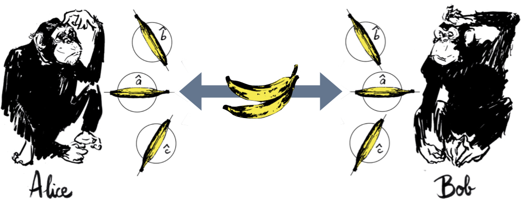
We focus on a species of banana that grows in pairs on special banana trees. These bananas can only taste yummy or nasty. Yet we cannot say that they come in two flavors, as they only acquire a definite flavor once they are peeled and tasted. We use these bananas in a long series of peel-and-taste experiments following a protocol familiar from experimental tests of Bell inequalities. We pick a pair of bananas, still joined at the stem, from the banana tree. We separate them and give one each to two chimps, Alice and Bob. Once they have received their respective bananas, they randomly and independently of one another pick a particular peeling, defined by the peeling direction, i.e., the direction of the line going from the top to the stem of the banana while it is being peeled. Alice and Bob are instructed not to change the orientation of their bananas while peeling so that it is unambiguous which peeling they are using. In the Mermin setup, Alice and Bob get to choose between three peelings, labeled $`\hat{a}`$, $`\hat{b}`$ and $`\hat{c}`$, represented by unit vectors, $`\vec{e}_a`$, $`\vec{e}_b`$ and $`\vec{e}_c`$, in the corresponding peeling directions (see Figure 1). Once they have randomly chosen one of these three peelings, they point the stem of their banana in the direction of the corresponding unit vector and peel their banana (it does not matter whether they peel from the top or from the stem). When done peeling, Alice and Bob reposition their bananas and take a bite to determine whether they taste yummy or nasty (see Figure 2). The whole procedure is then repeated with a fresh pair of bananas from the banana tree.
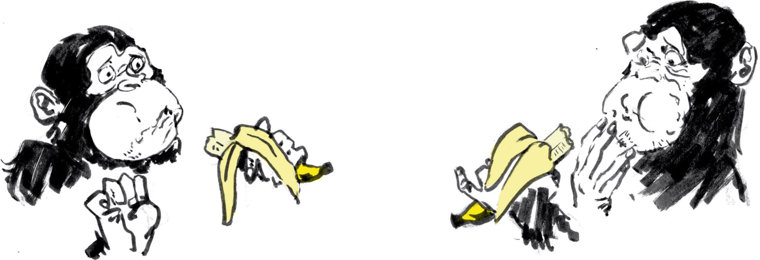
In each run of this peel-and-taste experiment, Alice and Bob record that run’s ordinal number, the peeling chosen ($`\hat{a}`$, $`\hat{b}`$ or $`\hat{c}`$) and the taste of their banana, using “$`+`$” for “yummy” and “$`-`$” for “nasty”. Every precaution is taken to ensure that, as long as there are more bananas to be peeled and tasted, Alice and Bob cannot communicate. While they are peeling and tasting, the only contact between them is that the bananas they are given come from pairs originally joined at the stem on the banana tree.
When all bananas are peeled and tasted, Alice and Bob are allowed to compare notes. Just looking at their own records, they see nothing out of the ordinary—just a sequence of pluses and minuses as random as if they had faked their results by tossing a coin for every run. Comparing their records, however, they note that, every time they happened to choose the same peeling (in roughly $`33 \%`$ of the total number of runs), their results are perfectly anti-correlated. Whenever one banana tasted yummy, its twin tasted nasty. In and of itself, this is not particularly puzzling. Maybe our bananas always grow in pairs in which one is predetermined to taste yummy while its twin is predetermined to taste nasty. This simple explanation, however, is ruled out by another striking correlation our chimps discover while pouring over their data. When they happened to peel differently (in roughly $`66 \%`$ of the runs), their results were positively correlated, albeit imperfectly. In 75% of the runs in which they used different peelings, their bananas tasted the same .49 The tastes of two bananas coming from one pair thus depend on the angle between the peeling directions used. This is certainly odd but one could still imagine that our bananas are somehow pre-programmed to respond differently to different peelings and that the set of pre-programmed responses is different for the two bananas in one pair. What Mermin’s Bell inequality shows, however, is that it is impossible to pre-program twin bananas in such a way that they would produce the specific correlations found in this case. Such correlations, however, can and have been produced with quantum twins (see Section 6.1). Given that they persist no matter how far we imagine Alice and Bob to be apart, another explanation of these curious correlations is also unavailing: it would take a signal traveling faster than the speed of light for the taste of one banana peeled a certain way to either affect the way the other banana is peeled or affect its taste when peeled that way. In short, these correlations cannot be accounted for on the basis of any local hidden-variable theory.
Non-signaling correlation arrays
The correlations found in the Mermin setup can be represented in a correlation array consisting of nine cells, one for each of the nine possible combinations of peelings (see Figure 6 in Section 2.3). These cells form a grid with three rows for Alice’s three peeling directions and three columns for Bob’s. Each cell has four entries, giving the probabilities of the four possible pairs of tastes for that cell’s combination of peelings (the entries in one cell thus always sum to 1).
Since Bananaworld focuses on setups with two settings per party, all correlation arrays in it have only four cells. These cells form a $`2 \times 2`$ grid with rows for Alice peeling from the stem and from the top and columns for Bob peeling from the stem and from the top. Before we turn to the $`3 \times 3`$ Mermin correlation array we go over some properties of these simpler $`2 \times 2`$ correlation arrays.
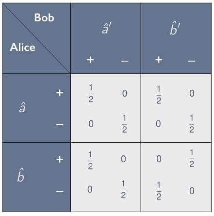
The correlation array in Figure 3 for a PR box in its original design is an example of such an array . This correlation array plays an important role in Bananaworld and is central to its sequel, Tanya and Jeffrey Bub’s (2018) enchanting Totally Random. A version of it is prominently displayed on many pages of this graphic novel . The version in Totally Random differs in two respects from the version in Figure 3 (which follows Bananaworld). First, in Figure 3, the outcomes found by Alice and Bob are perfectly correlated in three of the four cells, while they are perfectly anti-correlated in the remaining one. In Totally Random it is just the other way around. Second, instead of the four entries in each cell in Figure 3, the cells in Totally Random just have “$`=`$” for perfectly correlated and “$`\neq`$” for perfectly anti-correlated.
In Bananaworld the PR-box correlations in Figure 3 are realized with the help of PR bananas growing in pairs on PR banana trees. The settings $`\{\hat{a}, \hat{b}\}`$ and $`\{\hat{a}', \hat{b}'\}`$ now stand for Alice and Bob peeling their bananas from the stem ($`S`$) or from the top ($`T`$). These peelings could be replaced by two of the peeling directions we introduced. In realizations of this PR box, we can (but do not have to) use the same pair of settings for Alice and Bob (in the case of the CHSH setup we definitely need different pairs of settings; see Section 4).
In Totally Random, the PR-box correlations in Figure 3 are realized with the help of an imaginary device, named for the inventors of the PR box, the “Superquantum Entangler PR01”. This gadget, which looks like a toaster, has slots for two US quarters. When we insert two ordinary coins, the PR01 turns them into a pair of entangled “quoins” . The different settings now stand for Alice and Bob holding their quoins heads-up ($`\hat{a} = \hat{a}'`$) or tails-up ($`\hat{b} = \hat{b}'`$) when tossing them. The outcomes are the quoins landing heads or tails. What makes this a realization of a PR box with the correlation array shown in Figure 3 is that the quoins invariably land with the same side facing up, except when both are tossed being held tails-up ($`\hat{b}, \hat{b}'`$), in which case they always land with opposite sides facing up.
The correlations between the outcomes found in a PR box—be it between the tastes of a pair of PR bananas or the landings of a pair of quoins—are preserved no matter how far its two parts are pulled apart.50
An important feature of correlation arrays (no matter how many cells they have or how many entries each cell has) is that they allow us to see at a glance whether or not the correlations they represent can be used for the purposes of instant messaging or superluminal signaling. Suppose Alice wants to use the peeling of a pair of PR bananas to instant-message the answer to some “yes/no” question to Bob. They agree ahead of time that Alice will peel $`\hat{a}`$ if the answer is “yes” and $`\hat{b}`$ if it is “no”.51 This scheme will not work. No matter how Bob peels his banana, he cannot tell from its taste whether Alice peeled hers $`\hat{a}`$ or $`\hat{b}`$. Suppose Bob peels $`\hat{b}'`$ (essentially the same argument works if Bob peels $`\hat{a}'`$). In that case, the correlation array in Figure 3 tells us that the marginal probability of Bob finding $`+`$ if Alice were to peel $`\hat{a}`$ (trying to transmit “yes”) is
\begin{equation}
\mathrm{Pr}(+_{\mathrm B}| \hat{a} \,\hat{b}') = \mathrm{Pr}(+\!+| \hat{a} \,\hat{b}') \, + \, \mathrm{Pr}(-\!+| \hat{a} \,\hat{b}') =  \sfrac12 + 0 = \sfrac12,
\label{non-signaling property 1}
\end{equation}which is the same as the marginal probability of him finding $`+`$ if Alice were to peel $`\hat{b}`$ (trying to transmit “no”):
\begin{equation}
\mathrm{Pr}(+_{\mathrm B}| \hat{b} \,\hat{b}') = \mathrm{Pr}(+\!+| \hat{b} \,\hat{b}') \; + \; \mathrm{Pr}(-\!+| \hat{b} \,\hat{b}') =  0 + \sfrac12 = \sfrac12.
\label{non-signaling property 2}
\end{equation}Inspection of the correlation array in Figure 3 shows that all such marginal probabilities are equal to $`\sfrac12`$ in this case. PR boxes—whether realized with the help of magic bananas, quoins, or other systems—cannot be used for instant messaging.
Correlations that do not allow instant messaging are called non-signaling. It will be convenient to use this term for their correlation arrays as well. The correlations and correlation arrays for a PR box are always non-signaling. In fact, this is what makes these hypothetical devices intriguing. Even though they would give rise to correlations stronger than those allowed by quantum mechanics, they would not violate special relativity’s injunction against superluminal signaling.
Generalizing the results in Eqs. ([non-signaling property 1])–([non-signaling property 2]), we can state the following non-signaling condition:
A correlation in a setup with two parties, two settings per party and two outcomes per setting is non-signaling if the probabilities in both rows and both columns of all cells in its correlation array add up to $`\sfrac12`$.
The converse is not true. A correlation array with the entries
\begin{equation}
\begin{array}{cccc}
1  & 0  & 0 & 1 \\[.1 cm]
 0 & 0  & 0 & 0 \\[.1 cm]
 0 & 0  & 0 & 0 \\[.1 cm]
1 & 0 & 0 & 1
\end{array}
\end{equation}is non-signaling even though the entries in half the rows and columns of its cells add up to 1 while the entries in the other half add up to 0. The relevant marginal probabilities, however, are still equal to each other. For instance,
\begin{equation}
\mathrm{Pr}(+_{\mathrm B}|\hat{a} \,\hat{b}') = \mathrm{Pr}(+_{\mathrm B}|\hat{b} \,\hat{b}') = 0 \quad \mathrm{ and} \quad \mathrm{Pr}(-_{\mathrm B}|\hat{a} \,\hat{b}') = \mathrm{Pr}(-_{\mathrm B}|\hat{b} \,\hat{b}') = 1.
\end{equation}In Section 3, we will encounter correlation arrays for setups with three outcomes per setting that are non-signaling even though not all rows and columns of its cells add up to the same number (see Figure [CA-3set3out-raffle-vi] in Section 6.2.7).52
Non-signaling cubes, classical polytopes and the elliptope
Any cell in a non-signaling correlation array for any number of settings with two outcomes per setting can be parametrized by a variable with values running from $`-1`$ to $`+1`$. Figure 4 shows such a cell for Alice using setting $`\hat{a}`$ and Bob using setting $`\hat{b}`$. Let $`-1 \ge \chi_{ab} \ge 1`$ be the variable parametrizing this cell. If $`\chi_{ab} = 0`$, the results of Alice and Bob are uncorrelated; if $`\chi_{ab} =-1`$, they are perfectly correlated; if $`\chi_{ab} =1`$, they are perfectly anti-correlated. We will thus call $`\chi_{ab}`$ an anti-correlation coefficient.
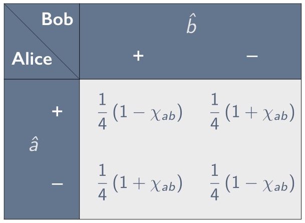
Consider the random variable $`X_a^A`$ measured by Alice using setting $`\hat{a}`$ and the random variable $`X_b^B`$ measured by Bob using setting $`\hat{b}`$. The covariance of these two variables is defined as the expectation value of the product of $`X_a^A - \langle X_a^A \rangle`$ and $`X_b^B - \langle X_b^B \rangle`$, where $`\langle X \rangle`$ is the expectation value of $`X`$:
\begin{equation}
\mathrm{cov} \! \left( X_a^A, X_b^B \right) \equiv \left\langle \left( X_a^A - \langle X_a^A \rangle \right) \left( X_b^B - \langle X_b^B \rangle \right) \right\rangle.
\label{cov def 0}
\end{equation}The random variables we will be considering are all balanced. That a random variable is balanced means that it has the following two properties:
A random variable $`X`$ is balanced IFF
MATH\begin{equation} \begin{array}{l} \text{(1) if $x$ is a possible value, then $-x$ is a possible value as well;} \\[.2cm] \text{(2) the value $x$ is as likely to occur as the value $-x$.} \end{array} \label{def balanced} \end{equation}Click to expand and view more
Such variables have zero expectation value, which means that Eq. ([cov def 0]) reduces to:
\begin{equation}
\mathrm{cov} \! \left( X_a^A, X_b^B \right) = \left\langle  X_a^A \, X_b^B \right\rangle.
\label{cov def}
\end{equation}Bell inequalities (including the CHSH one) are typically expressed in terms of such expectation values. To compute $`\langle X_a^A \, X_b^B \rangle`$, we need to assign a numerical value to the taste of a banana. To this end, we introduce the Bub or banana constant $`b`$. Yummy ($`+`$) and nasty ($`-`$) then correspond to $`\pm \bbar/2`$, where $`\bbar \equiv b/2\pi`$ (called banana split or banana bar). Using the entries in the correlation array in Figure 4, we evaluate the expectation value of the product of $`X_a^A`$ and $`X_b^B`$:
\begin{eqnarray}
\left\langle X_a^A \, X_b^B \right\rangle & = & \frac{\bbar^2}{4} \left(\mathrm{Pr}(+\!+| \hat{a} \,\hat{b}) \, + \, \mathrm{Pr}(-\!-| \hat{a} \,\hat{b})\right)
- \frac{\bbar^2}{4} \left(\mathrm{Pr}(+\!-| \hat{a} \,\hat{b}) \, + \, \mathrm{Pr}(-\!+| \hat{a} \,\hat{b})\right) \nonumber \\[.2 cm]
& = & \frac{\bbar^2}{4} \left( \frac12 (1 - \chi_{ab}) - \frac12 (1 + \chi_{ab}) \right) \; = \; -\frac{\bbar^2}{4} \chi_{ab}.
\label{prob 2 exp}
\end{eqnarray}Introducing the standard deviations of $`X_a^A`$ and $`X_b^B`$,
\begin{equation}
\begin{array}{c}
\sigma^A_a \equiv \sqrt{ \left\langle (X^A_a)^2 - \langle X_a^A \rangle^2 \right\rangle} = \sqrt{ \left\langle (X^A_a)^2 \right\rangle }= \displaystyle{\frac{\bbar}{2}},    \\[.4cm]
\sigma^B_b \equiv  \sqrt{ \left\langle (X^B_b)^2 - \langle X_b^B \rangle^2 \right\rangle} = \sqrt{ \left\langle (X^B_b)^2 \right\rangle }= \displaystyle{\frac{\bbar}{2}}
\end{array}
\label{standard deviations a and b}
\end{equation}where we used that $`\langle X_a^A \rangle = \langle X_b^B \rangle = 0`$, we can thus write the parameter $`\chi_{ab}`$ introduced in Figure 4 as
\begin{equation}
\chi_{ab} = - \frac{\left\langle X_a^A \, X_b^B \right\rangle}{\sigma^A_a \sigma^B_b}.
\label{chi as corr coef}
\end{equation}This is our formal justification for calling $`\chi_{ab}`$ (and parameters like it for other cells in this and other correlation arrays) an anti-correlation coefficient: it is minus what is commonly known as Pearson’s correlation coefficient. We will return to this information-theoretic interpretation of $`\chi_{ab}`$ in Section 6.2.
 style="width:5in" />
A $`2 \times 2`$ non-signaling correlation array such as the one in Figure 3 for a PR box, with four cells of the form of Figure 4, can be parametrized by four anti-correlation coefficients
\begin{equation}
-1 \le \chi_{aa'} \le 1, \quad -1 \le \chi_{ab'} \le 1, \quad -1 \le \chi_{ba'} \le 1, \quad -1 \le \chi_{bb'} \le 1.
\label{chi values for PR box}
\end{equation}Such a correlation array can thus be represented by a point in a hypercube in four dimensions with the anti-correlation coefficients serving as that point’s Cartesian coordinates. The correlation array for a PR box is represented by one of the vertices of this hypercube:
\begin{equation}
(\chi_{aa'}, \chi_{ab'}, \chi_{ba'}, \chi_{bb'}) = (-1, -1, -1, 1).
\label{PR box vertices}
\end{equation}The four-dimensional hypercube that represents the class of all non-signaling correlations in this setup (two parties, two settings per party, two outcomes per setting) is an example of a so-called non-signaling polytope, which can be defined (typically in some higher-dimensional space) for setups with two parties, any number of settings and any number of outcomes per setting.

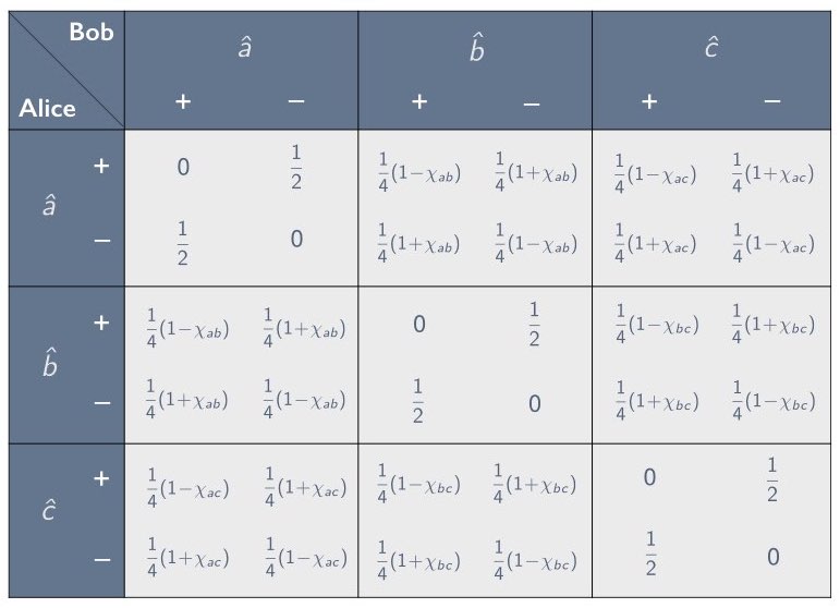
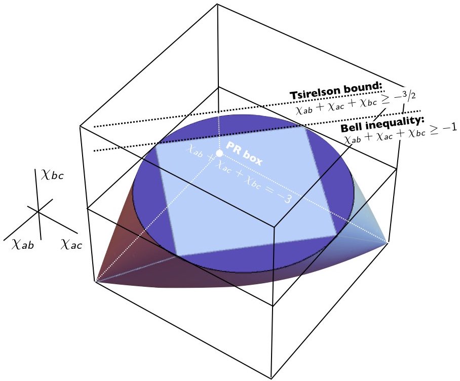
Figure 5 gives a schematic representation of the non-signaling polytope for such a setup. The outer square and everything inside of it (the non-signaling polytope $`\mathcal{P}`$) represents the set of all non-signaling correlations. The inner square and everything inside of it (the local polytope $`\mathcal{L}`$) represents the set of all non-signaling correlations allowed classically (i.e., by a local hidden-variable theory). The circle in between these two squares and everything inside of it (the quantum convex set $`\mathcal{Q}`$) represents the set of all correlations allowed quantum-mechanically. One of the facets of $`\mathcal{L}`$ represents a Bell inequality, a bound on the strength of the correlations allowed classically. The vertex of the non-signaling cube where this bound is maximally violated represents a PR box for the setup under consideration.
Figure 6 shows the correlation array for our version of Mermin’s example of a quantum correlation violating a Bell inequality. We will refer to it as the Mermin correlation array. Its nine cells form a $`3 \times 3`$ grid. The cells along the diagonal of this grid, when Alice and Bob peel the same way, show a perfect anti-correlation. The six off-diagonal cells, when Alice and Bob peel differently, all show the same imperfect positive correlation. It is easy to see that this correlation array is non-signaling: the entries in both rows and both columns of all nine cells add up to $`\sfrac12`$. Concisely put, this correlation (array) has uniform marginals.
The Mermin correlation array in Figure 6 is a special case of the more general correlation array in Figure 7. The three cells along the diagonal are the same, all showing a perfect anti-correlation (i.e., its diagonal elements are 0 and its off-diagonal elements are $`\sfrac12`$). Moreover, cells on opposite sides of the diagonal are the same. This correlation array can thus be parametrized by three anti-correlation coefficients of the kind introduced in Figure 4 and Eq. ([chi as corr coef]). In the specific example of the Mermin setup in Figure 6, the three anti-correlation coefficients have the same value:
\begin{equation}
\chi_{ab} = \chi_{ac} = \chi_{bc} = -\sfrac12.
\label{chi values Mermin example}
\end{equation}The class of all non-signaling correlations in the Mermin setup can be visualized as a cube in ordinary three-dimensional space with the correlation coefficients, $`\chi_{ab}`$, $`\chi_{ac}`$ and $`\chi_{bc}`$, providing the three Cartesian coordinates of points in this cube. The non-signaling correlations allowed classically can be represented by a tetrahedron spanned by four of the eight vertices of this non-signaling cube (see Figure 14 in Section 2.4); those allowed quantum-mechanically by an elliptope enclosing this tetrahedron (see Figure [elliptope] in Section 6.1). Figure 8 shows the cross-section $`\chi_{bc} =0`$ of this non-signaling cube, the classical tetrahedron and the elliptope. This cross-section has exactly the form of the cartoonish rendering in Figure 5 of the Vitruvian-man-like structure of the local polytope $`\mathcal{L}`$ and the quantum convex set $`\mathcal{Q}`$ inside the non-signaling polytope $`\mathcal{P}`$. In the next two subsections, we will show in detail how one arrives at the classical tetrahedron and the quantum elliptope in the Mermin setup.
Classical polytopes and raffles to simulate quantum correlations
As explains in the opening chapter of Bananaworld, to decide whether or not some correlation array is allowed classically (or quantum-mechanically), he checks whether or not it can be simulated with classical (or quantum-mechanical) resources. Though we will use a more direct approach to find classes of correlations allowed quantum-mechanically (see Sections 6.1 and 3.1), we will adopt a variation on Bub’s imitation game to find classes of correlations allowed classically (i.e., by some local hidden-variable theory).
We will use special raffles to simulate the correlations found in our quantum banana peeling and tasting experiments. These raffles involve baskets of tickets such as the ones in Figure 10. All tickets list the outcomes for both parties and for all settings in the setup under consideration. We randomly draw a ticket of the appropriate kind from a basket with many such tickets. We tear this ticket in half and randomly decide which side goes to Alice and which side goes to Bob. Alice and Bob then decide, randomly and independently of each other, which setting they will use. They record the outcome for that setting printed on their half of the ticket. We repeat this procedure a great many times.
Raffles of this kind provide a criterion for determining whether or not a certain correlation is allowed classically:53
A correlation array is allowed by a local hidden-variable theory if and only if there is a raffle (i.e., a basket with the appropriate mix of tickets) with which we can simulate that correlation array following the protocol described above.
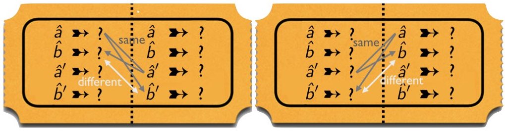
Invoking this criterion, we can easily show that a PR box with the correlation array in Figure 3 is not allowed classically.54 These correlations place impossible demands on the design of the tickets for a raffle that would simulate them (see Figure 9). The perfect positive correlation between the outcomes for three of the four possible combinations of settings ($`\hat{a} \, \hat{a}'`$, $`\hat{a} \, \hat{b}'`$ and $`\hat{b} \, \hat{a}'`$) requires that the outcomes printed on the ticket for $`\hat{a}`$ and $`\hat{b}`$ on one side are the same as the outcomes for $`\hat{a}'`$ and $`\hat{b}'`$ on the other side. That makes it impossible for the outcomes for $`\hat{b}`$ and $`\hat{b}'`$ on opposite sides of the ticket to be different as required by the perfect anti-correlation for the remaining combination of settings ($`\hat{b} \, \hat{b}'`$).
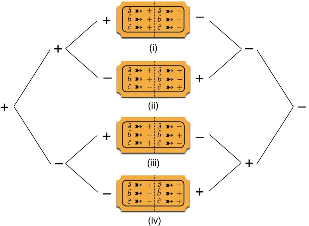
Figure 10 shows four different types of tickets, labeled (i) through (iv), for raffles meant to simulate correlations found in the Mermin setup in which Alice and Bob choose from the same three settings $`(\hat{a}, \hat{b}, \hat{c})`$ with two possible outcomes each $`(+, -)`$. Since in all setups that we will examine Alice and Bob find opposite results whenever they use the same setting, the outcomes on one side of the ticket dictate the outcomes on the other. That reduces the number of different ticket types to $`2^3 = 8`$. Given that it is decided randomly which side of a ticket goes to Alice and which side to Bob, two tickets that differ only in that the left and the right side are swapped are two equivalent versions of the same ticket type. This further reduces the number of different ticket types to four. As illustrated in Figure 10, we chose the ones that have $`+`$ for the first setting ($`\hat{a}`$) on the left side of the ticket.
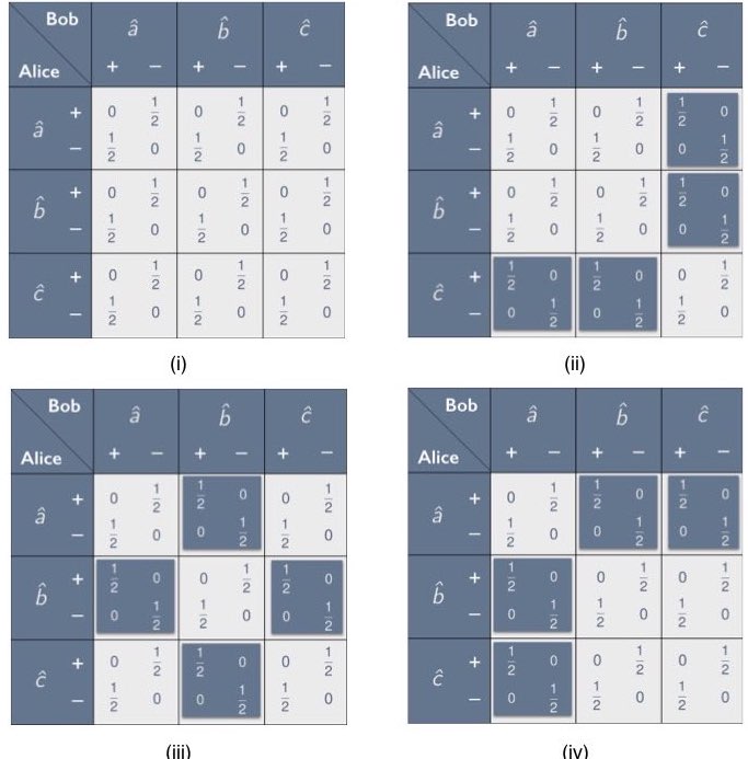
Figure 11 shows the correlation arrays for raffles with baskets containing only one of the four types of tickets in Figure 10. The design of our raffles guarantees that the correlations between the outcomes found by Alice and Bob are non-signaling. This is borne out by the correlation arrays in Figure 11. The entries in both rows and both columns of all cells in these correlation arrays add up to $`\sfrac12`$. In other words, these raffles all give uniform marginals. The design of our raffle tickets also guarantees that the outcomes found by Alice and Bob are balanced (see the definition in the sentence following Eq. ([cov def 0])).
The entries of correlation arrays like those in Figure 11 form $`6 \times 6`$ matrices. These matrices are symmetric. This is true both for single-ticket and mixed raffles. All raffles we will consider have this property. This too follows directly from the design of these raffles. It is simply because Alice and Bob are as likely to get the left or the right side of any ticket.
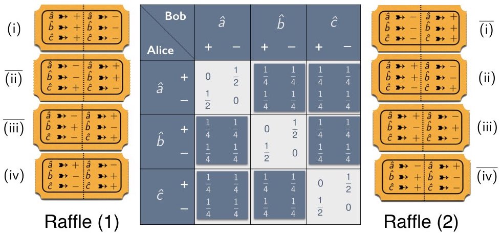
Before we continue our analysis, we show that changing the protocol of our raffles so that Alice is always given the left side and Bob is always given the right side of any ticket does not give rise to correlation arrays with symmetric associated matrices that cannot be simulated with our more economical protocol—more economical because it requires fewer ticket types. For the alternative protocol, we need four more tickets, labeled $`\overline{(\mathrm{i})}`$ through $`\overline{(\mathrm{iv})}`$, that differ from their counterparts (i) through (iv) in that the left and right sides of the ticket have been swapped. Figure 12 shows two raffles for this alternative protocol. Raffle (1) has equal numbers of tickets of type $`\big\{ \mathrm{(i)}, \overline{(\mathrm{ii})}, \overline{(\mathrm{iii})}, \mathrm{(iv)} \big\}`$. The matrix associated with the correlation array for this raffle is symmetric. That means that we get the same correlation array if we swap the left and the right sides of all tickets in raffle (1). This turns raffle (1) into raffle (2) with equal numbers of tickets of type $`\big\{ \overline{(\mathrm{i})}, \mathrm{(ii)}, \mathrm{(iii)}, \overline{(\mathrm{iv})} \big\}`$. Any raffle mixing raffles (1) and (2) will also give that same correlation array. Consider the special case of a raffle with equal numbers of all eight tickets. This raffle is equivalent to a basket with equal numbers of tickets $`\big\{ \mathrm{(i)}, \mathrm{(ii)}, \mathrm{(iii)}, \mathrm{(iv)} \big\}`$ with the understanding that it is decided at random which side of the ticket goes to Alice and which side goes to Bob. This construction works for any correlation array with a symmetric associated matrix that we can produce using the protocol in which Alice always get the left side and Bob always get the right side of a ticket. We conclude that we can produce any such correlation array using our more economical protocol.
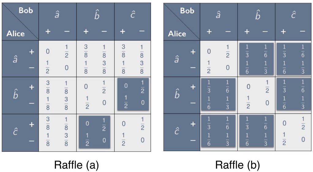
There is no mix of tickets (i) through (iv) in Figure 10 that produces a raffle that can simulate the Mermin correlation array in Figure 6. Figure 13 shows the results of two unsuccessful attempts to produce one. In the first, we take a basket with 25% tickets of type (i) and 75% of type (iv). This results in correlation array (a) in Figure 13. This raffle correctly simulates all but two cells of the Mermin correlation array. We get the same result if we replace tickets (iv) by tickets (ii) or (iii), the only difference being that now two other cells will differ from the corresponding ones in the Mermin correlation array. The best we can do overall is to take a basket with 33% each of tickets (ii) through (iv). This results in correlation array (b) in Figure 13. Like the Mermin correlation array we are trying to simulate, this one has the same positive correlation in all six off-diagonal cells but the correlation is weaker ($`-\chi_{ab} = -\chi_{ac} = -\chi_{bc} = \sfrac13`$) than in the Mermin case ($`-\chi_{ab} =-\chi_{ac} = -\chi_{bc} = \sfrac12`$).
To prove that there is no raffle that can simulate the Mermin correlation array, we consider the sum $`\chi_{ab} + \chi_{ac} + \chi_{bc}`$ of the anti-correlation coefficients for a raffle. From the tickets in Figure 10 we can read off the values of $`\chi_{ab}`$, $`\chi_{ac}`$ and $`\chi_{bc}`$ for the four single-ticket raffles. These values are brought together in Table 1.
| ticket | $`\chi_{ab}`$ | $`\chi_{ac}`$ | $`\chi_{bc}`$ |
|---|---|---|---|
| (i) | $`+1`$ | $`+1`$ | $`+1`$ |
| (ii) | $`+1`$ | $`-1`$ | $`-1`$ |
| (iii) | $`-1`$ | $`+1`$ | $`-1`$ |
| (iv) | $`-1`$ | $`-1`$ | $`+1`$ |
Values of the anti-correlation coefficients parametrizing the off-diagonal cells of the correlation arrays (i) through (iv) in Figure 11 for single-ticket raffles with tickets (i) through (iv) in Figure 10.
The cells in the correlation arrays in Figure 11 are all either perfectly anti-correlated or perfectly correlated. The anti-correlation coefficients for these single-ticket raffles can therefore only take on the values $`\pm 1`$ and their sum can only take on the value 3 (for a raffle with tickets of type (i) only) or $`-1`$ (for raffles with tickets (ii) or (iii) or (iv) only). For mixed raffles, $`\chi_{ab} + \chi_{ac} + \chi_{bc}`$ is the weighted average of the value of $`\chi_{ab} + \chi_{ac} + \chi_{bc}`$ for these four single-ticket raffles, with the weights given by the fractions of each of the four tickets in the raffle.55 Hence, for any mix of tickets, this sum must lie between $`-1`$ and $`3`$:
\begin{equation}
-1 \le \chi_{ab} + \chi_{ac} + \chi_{bc} \le 3.
\label{Mermin inequality CHSH-like}
\end{equation}The first of these inequalities, giving the lower bound on $`\chi_{ab} + \chi_{ac} + \chi_{bc}`$, is the analogue of the CHSH inequality for our variation of the Mermin setup. It is also the form in which originally derived the Bell inequality. The CHSH-type Bell inequality is violated by the Mermin correlation array in Figure 6. In that case, $`\chi_{ab} = \chi_{ac} = \chi_{bc} = - \sfrac12`$ (see Eq. ([chi values Mermin example])) and their sum equals $`-\sfrac32`$. As we will see in Section 6.1, this is the maximum violation of this inequality allowed by quantum mechanics. Note that the absolute minimum value of $`\chi_{ab} + \chi_{ac} + \chi_{bc}`$ is $`-3`$. This value is allowed neither classically nor quantum-mechanically. It is the value reached with the (hypothetical) PR box for this setup.
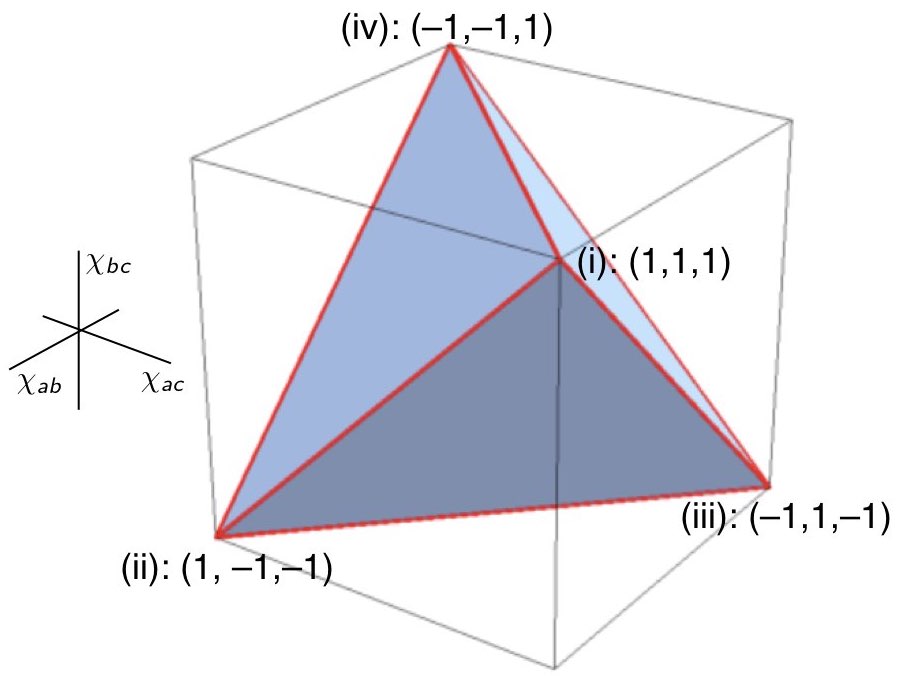
The values of $`\chi_{ab}`$, $`\chi_{ac}`$ and $`\chi_{bc}`$ in Table 1 for tickets (i) through (iv) can be used as the Cartesian coordinates of four vertices in the non-signaling cube for the Mermin setup. These are the vertices labeled (i) through (iv) in Figure 14. The vertex $`(-1, -1, -1)`$ represents the PR box for this setup (see Figure 8). The vertices (i) through (iv) span a tetrahedron forming the convex set of all raffles that can be obtained by mixing the four types of tickets. The sum $`\chi_{ab} + \chi_{ac} + \chi_{bc}`$ takes on its maximum value of 3 at the vertex for tickets of type (i) and its minimum value of $`-1`$ for the facet spanned by the vertices for tickets of types (ii), (iii) and (iv). The inequalities in Eq. ([Mermin inequality CHSH-like]) tell us that all correlations that can be simulated with raffles with various mixes of tickets must lie in the region of the non-signaling cube between the vertex (i) and the facet (ii)-(iii)-(iv).
This is a necessary but not a sufficient condition for a correlation to be allowed by a local hidden-variable theory. As Figure 14 shows, there are three forbidden sub-regions in the region between vertex (i) and facet (ii)-(iii)-(iv). A full characterization of the class of correlations allowed classically requires three additional pairs of inequalities like the pair given in Eq. ([Mermin inequality CHSH-like]), corresponding to the other three vertices and the other three facets of the tetrahedron. The following four pairs of inequalities do fully characterize the tetrahedron:
\begin{eqnarray}
-1 \le \;\, \chi_{ab} + \chi_{ac} + \chi_{bc} \; \le 3  & \!\!\!\! & \textrm{[between facet (ii)-(iii)-(iv) and vertex (i)]}
\label{Mermin inequality CHSH-like (i)} \\[.4cm]
-1 \le \;\, \chi_{ab} - \chi_{ac} - \chi_{bc} \; \le 3  & \!\!\!\!  & \textrm{[between facet (i)-(iii)-(iv) and vertex (ii)]}
\label{Mermin inequality CHSH-like (ii)} \\[.4cm]
-1 \le - \chi_{ab} + \chi_{ac} - \chi_{bc} \le 3 & \!\!\!\!  & \textrm{[between facet (i)-(ii)-(iv) and vertex (iii)]}
\label{Mermin inequality CHSH-like (iii)} \\[.4cm]
-1 \le - \chi_{ab} - \chi_{ac} + \chi_{bc} \le 3 & \!\!\!\!   & \textrm{[between facet (i)-(ii)-(iii) and vertex (iv)]}.
\label{Mermin inequality CHSH-like (iv)}
\end{eqnarray}Using the symmetries of the tetrahedron we can easily get from any one of these pairs of inequalities to another. Another way to see this is to recall that the coordinates $`(\chi_{ab}, \chi_{ac}, \chi_{bc})`$ are anti-correlation coefficients for different combinations of the measurement settings $`(\hat{a}, \hat{b}, \hat{c})`$ and to look at what happens when we flip the sign of the outcomes for one of these three settings. If we do this for $`\hat{a}`$, $`\chi_{ab}`$ and $`\chi_{ac}`$ pick up a minus sign and Eq. ([Mermin inequality CHSH-like (i)]) turns into Eq. ([Mermin inequality CHSH-like (iv)]). If we do this for $`\hat{b}`$, $`\chi_{ab}`$ and $`\chi_{bc}`$ pick up a minus sign and Eq. ([Mermin inequality CHSH-like (i)]) turns into Eq. ([Mermin inequality CHSH-like (iii)]). Finally, if we do this for $`\hat{c}`$, $`\chi_{ac}`$ and $`\chi_{bc}`$ pick up a minus sign and Eq. ([Mermin inequality CHSH-like (i)]) turns into Eq. ([Mermin inequality CHSH-like (ii)]).
Mermin formulated a different inequality for this setup, one that implies the lower bound on the sum of anti-correlation coefficients in Eq. ([Mermin inequality CHSH-like]) but requires an additional assumption. To derive Mermin’s inequality, we have to assume that Alice and Bob randomly and independently of each other decide which setting to use in any run of the experiment (whether with raffle tickets, spin-$`\frac12`$ particles, or quantum bananas). This provision is part of the protocol we described in Section 2.1 but we had no need to invoke it so far. The CHSH-like inequality in Eq. ([Mermin inequality CHSH-like]) could be derived without it—and so, for that matter, can the CHSH inequality itself.
This means that we can test these inequalities without having to change the settings in every run. We can make measurements for one pair of settings at a time, providing data for the correlation array one cell at a time. This is how originally tested the CHSH inequality. Changing the orientation of their polarizers was a cumbersome process.56 Because of this limitation of their equipment, the violation of the CHSH inequality they found could conceivably be blamed on the two photons generated as an entangled pair “knowing” ahead of time (i.e., the moment they separated) what the orientation of the polarizers would be with which they were going to be measured. To close this loophole, the settings should only be chosen once the photons are in flight. This was accomplished by Aspect and his collaborators later in the 1970s and in the 1980s . In this paper, we will not be concerned with the extensive experimental efforts to close this and other loopholes.57
If we assume that Alice and Bob randomly and independently of each other decide which setting to use in each run,58 the nine possible combinations of settings are equiprobable. Following , we ask for the probability, $`\mathrm{Pr(opp)}`$, that Alice and Bob find opposite results. Consider the Mermin correlation array in Figure 6. For the cells along the diagonal $`\mathrm{Pr(opp)} = 1`$ (the results are perfectly anti-correlated). For the off-diagonal cells $`\mathrm{Pr(opp)} = \sfrac14`$, the sum of the off-diagonal entries in those cells. Alice and Bob use the same setting in one out of three runs and different settings in two out of three. Hence, the probability of them finding opposite results is:
\begin{equation}
\mathrm{Pr(opp)} = \sfrac13 \cdot 1 \, + \, \sfrac23 \cdot \sfrac14 = \sfrac12.
\label{Pr opp Mermin}
\end{equation}Upon inspection of the four correlation arrays in Figure 11, however, we see that the minimum value for $`\mathrm{Pr(opp)}`$ in a local hidden variable theory is $`\sfrac59`$. In correlation array (i), the results in all nine cells are perfectly anti-correlated. In a single-ticket raffle with tickets of type (i), we thus have $`\mathrm{Pr(opp)} = 1`$. In each of the other three correlation arrays, there are five cells in which the results are perfectly anti-correlated and four in which they are perfectly correlated. In single-ticket raffles with tickets of type (ii), (iii), or (iv), we thus have $`\mathrm{Pr(opp)} = \sfrac59`$. For an arbitrary mix of tickets (i) through (iv), we therefore have the inequality
\begin{equation}
\mathrm{Pr(opp)} \ge \sfrac59.
\label{Mermin inequality probs}
\end{equation}This is the form in which Mermin states the Bell inequality for the setup we are considering. It implies the lower bound in Eq. ([Mermin inequality CHSH-like]). Consider, once again, the general non-signaling correlation array in Figure 7 parametrized by the anti-correlation coefficients $`\chi_{ab}`$, $`\chi_{ac}`$ and $`\chi_{bc}`$. Adding the off-diagonal elements in every cell and dividing by 9, as we are assuming that Alice and Bob use the settings of all nine cells with equal probability, we find
\begin{eqnarray}
\mathrm{Pr(opp)} & \!\! = \!\! & \sfrac39 \, + \, \sfrac29 \cdot \sfrac12 \, \Big(1+ \chi_{ab} \Big) \, + \, \sfrac29 \cdot \sfrac12 \, \Big(1+ \chi_{ac} \Big) \, + \,  \sfrac29 \cdot \sfrac12 \, \Big(1+ \chi_{bc} \Big) \nonumber \\[.2cm]
 & \!\! = \!\!  & \sfrac{2}{3} \, + \, \sfrac{1}{9} \, \Big(\chi_{ab} + \chi_{ac} + \chi_{bc} \Big).
 \label{Pr opp general}
\end{eqnarray}If $`\mathrm{Pr(opp)}`$ must at least be $`\sfrac59`$, then $`\chi_{ab} + \chi_{ac} + \chi_{bc}`$ cannot be smaller than $`-1`$. Conversely, if $`\chi_{ab} + \chi_{ac} + \chi_{bc} \ge -1`$ and all nine combinations of the settings $`\hat{a}`$, $`\hat{b}`$ and $`\hat{c}`$ are equiprobable, then $`\mathrm{Pr(opp)} \ge \sfrac59`$.
Mermin’s lower bound on the probability of finding opposite results may be easier to grasp for a general audience than a lower bound on a sum of expectation values. The latter, however, does have its own advantages. First, as we just saw, it can be derived from weaker premises. Second, it immediately generates inequalities corresponding to other facets of the polyhedron of classically allowed correlations in the Mermin setup (see Eqs. ([Mermin inequality CHSH-like (i)])–([Mermin inequality CHSH-like (iv)])). Third, as we will show in detail in Section 4, it makes it easier to see the connection with the CHSH inequality.
We noted in Section 1 that for Heisenberg, quantum mechanics’ significance lay in its provision of a new framework for doing physics, one that was sorely needed in light of the persistent failures of classical mechanics and the old quantum theory of Bohr and Sommerfeld to deal with the puzzling (mostly spectroscopic) experimental data it was confronted with in the first two decades of the last century . Heisenberg’s core insight into quantum mechanics’ significance is one that we and the others close to us on the phylogenetic tree of interpretations share. In the body of this paper we saw a number of concrete examples vividly illustrating the essential differences between the quantum and the classical kinematical framework, how those differences are manifested in the correlations between and in the dynamics of quantum systems, and finally how the quantum-kinematical framework enables us to learn about the specifics of particular systems through measurement. In this final section we present our view in a nutshell.
Quantum mechanics is about probabilities. The kinematical framework of the theory is probabilistic in the sense that the state specification of a given system yields, in general, only the probability that a selected observable will take on a particular value when we query the system concerning it. Quantum mechanics’ kinematical framework is also non-Boolean: The Boolean algebras corresponding to the individual observables associated with a given system cannot be embedded into a global Boolean algebra comprising them all, and thus the values of these observables cannot (at least not straightforwardly) be taken to represent the properties possessed by that system in advance of their determination through measurement. It is in this latter—non-Boolean—aspect of the probabilistic quantum-kinematical framework that its departure from classicality can most essentially be located.
Despite this character, we have seen above how the quantum-mechanical framework provides a recipe59 through which one can acquire information concerning particular systems by classical means. Given an ensemble of quantum systems either prepared uniformly in a particular state $`| \psi \rangle`$ or as a mixture of states $`| \psi \rangle_i`$ (described by the density operators $`\hat{\rho} = | \psi \rangle\langle \psi |`$ and $`\hat{\rho} = \sum_i| \psi \rangle_{\!i} \, _{i\!}\langle \psi |`$, respectively), and conditional upon a particular classically describable assessment of one of the parameters of the systems in that ensemble—conditional, that is, upon a particular Boolean frame that we impose on those systems—the information we obtain from our assessment can always be (re)described as having arisen from an ensemble of classical systems (like the raffles in our examples) with a certain distribution of values for the parameter in question. Further, the particular distribution observed can be predicted from the quantum state.
This recipe does not solve the profound problem of measurement; i.e., the problem to account for how it is that only some of the classical probability distributions implicit in the quantum state description are actualized in the context of a given measurement. But even without providing an answer to this question, we see how the kinematical core of quantum mechanics provides us with all of the tools we need to give an account of the dynamics of a particular measurement interaction, and through this explain why a particular classical probability distribution can be used to characterize the statistics observed within that measurement context, despite the non-classical nature of the quantum state description.
It may be objected that the world we experience does not consist in probability distributions. Its objects include this table, that banana and the other dynamical objects we observe and interact with, both in the kitchens of the world and outside of them, every day. These objects will not be found within the quantum-kinematical framework, nor will the recipe just mentioned yield them up in and of itself. Conditional upon a given measurement, however, that recipe will allow one to transition from the quantum description of a system to the classical description of the observations which ensue. And from there we already know how to use classical theory to construct, from these observations, the familiar objects of our world.
As our examples have demonstrated, quantum theory is successful where classical theory falls short in its description of physical phenomena, and its advent has uncovered aspects of our world that were before then veiled in darkness. But besides these particular lessons there is a wider moral that we can glean from the new kinematical framework of quantum theory, and in particular by considering how it differs from classical theory. The logical framework of classical physics is a globally Boolean structure. Through it a global noncontextual assignment of values to the observables associated with physical systems becomes possible. Because of this, these value assignments may unproblematically be thought of as the underlying properties of the physical systems they have been assigned to. This allows us to speak of a world that exists in a particular way irrespective of our particular interactions with it. Quantum mechanics, however, shows us that this classical description is valid only up to a certain point, and that the logical structure of the world as it presents itself to us is globally non-Boolean. Whatever else we may discover in the course of the future development of physical theory, this is a non-trivial fact that we have discovered about the world. Moreover it is a fact that will remain with us . It is, further, a non-trivial fact that we can learn about our world, despite this non-Boolean character, through classical means .60
It will be objected that what we have just called “facts about the world” are really only relational facts about our connection to the world . This is entirely correct. But that, we maintain, is how it should be. For we are entangled with the world, and our concepts both of the world and of ourselves are only marginals of that true entangled description. That description, along with its many seemingly incompatible aspects, arises out of and is made possible through the non-Boolean probabilistic structure of the quantum-mechanical kinematical core.
Quantum theory provides us with an objective description of a given system. This description is valid irrespective of one’s particular choices and irrespective of one’s particular interests in making those choices. At the same time the description that quantum theory provides to us of a given system’s dynamical state is unlike the corresponding description given to us by classical theory. In quantum theory, what is exhibited to us through the quantum state description is not the set of dynamical properties, in the classical sense, of the system of interest. What is exhibited, rather, is the structure of, interrelations between, and interdependencies among the possible perspectives one can take on that system. In this way quantum theory informs us regarding the structure of the world—a world that includes ourselves—and of our place within that structure.
📊 논문 시각자료 (Figures)
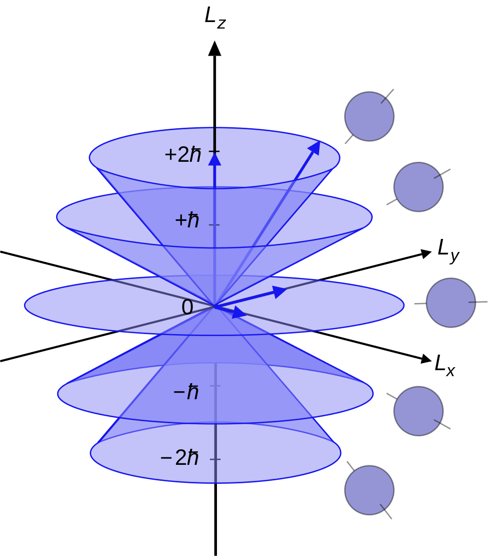
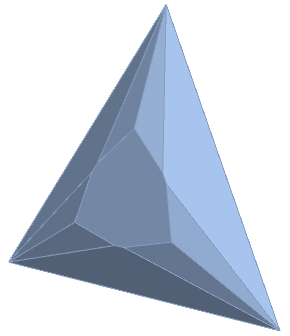
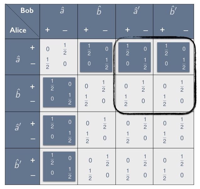
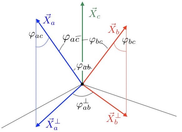
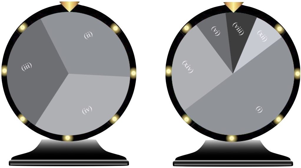
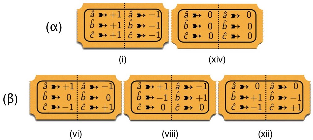
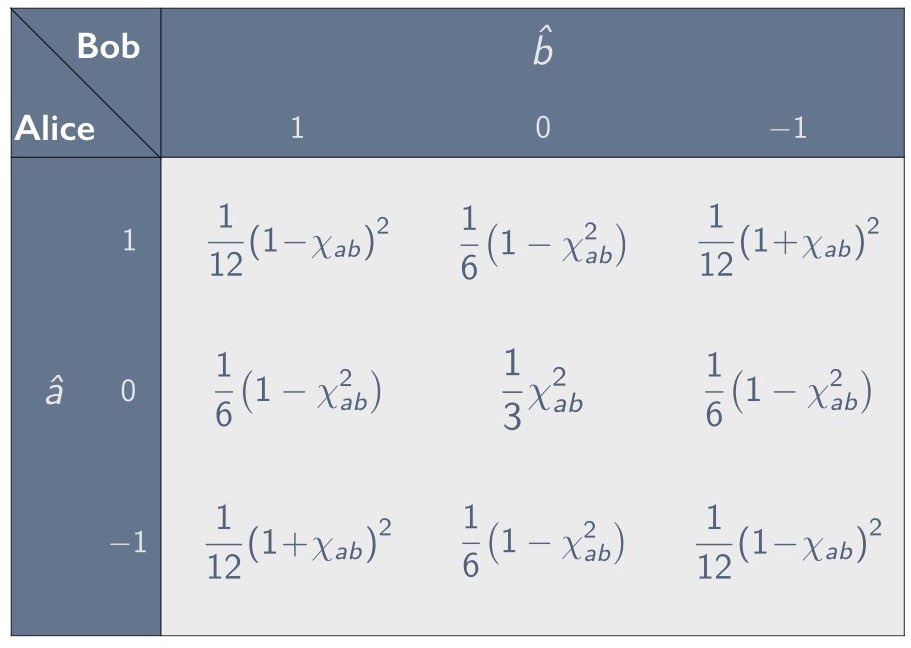
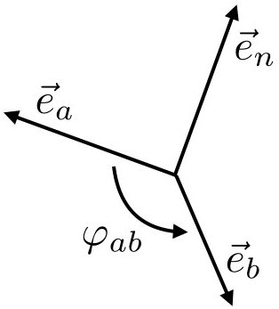
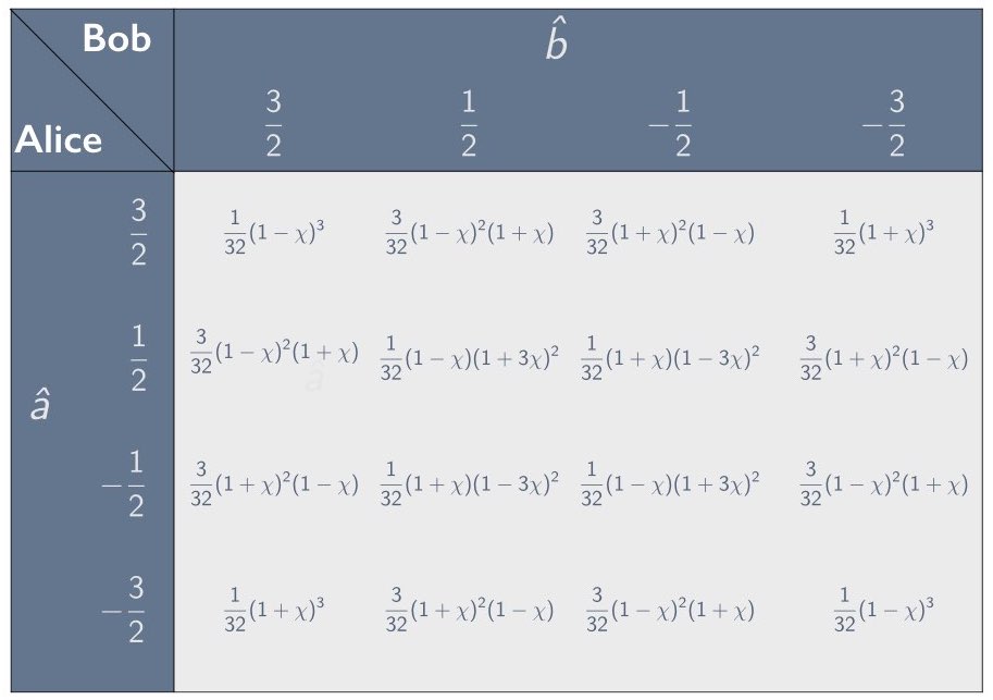
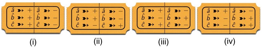
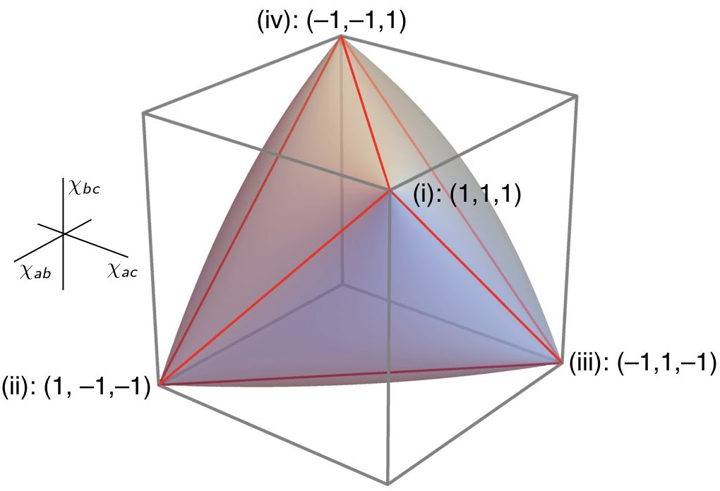
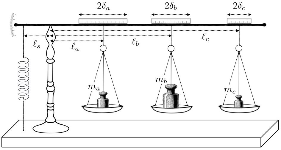
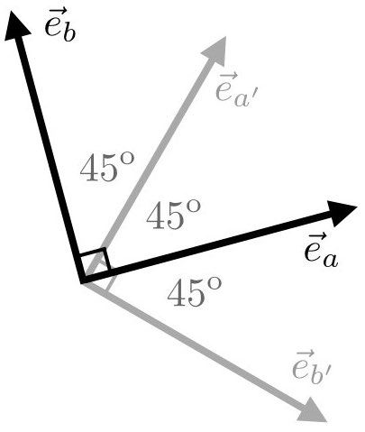

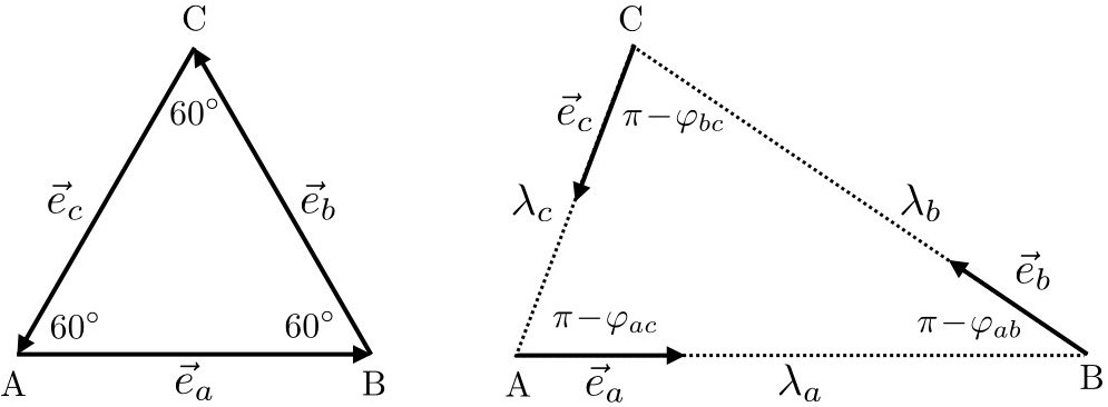
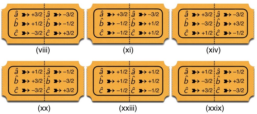
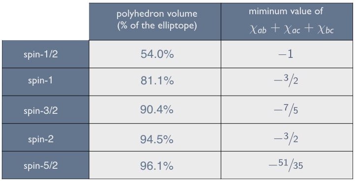
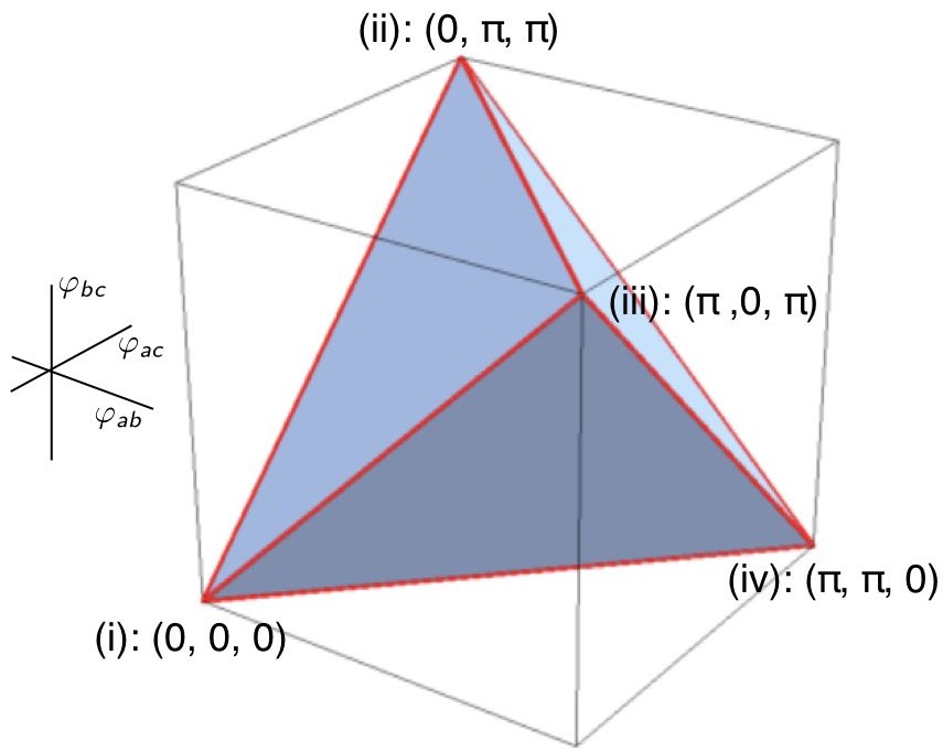
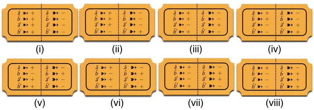
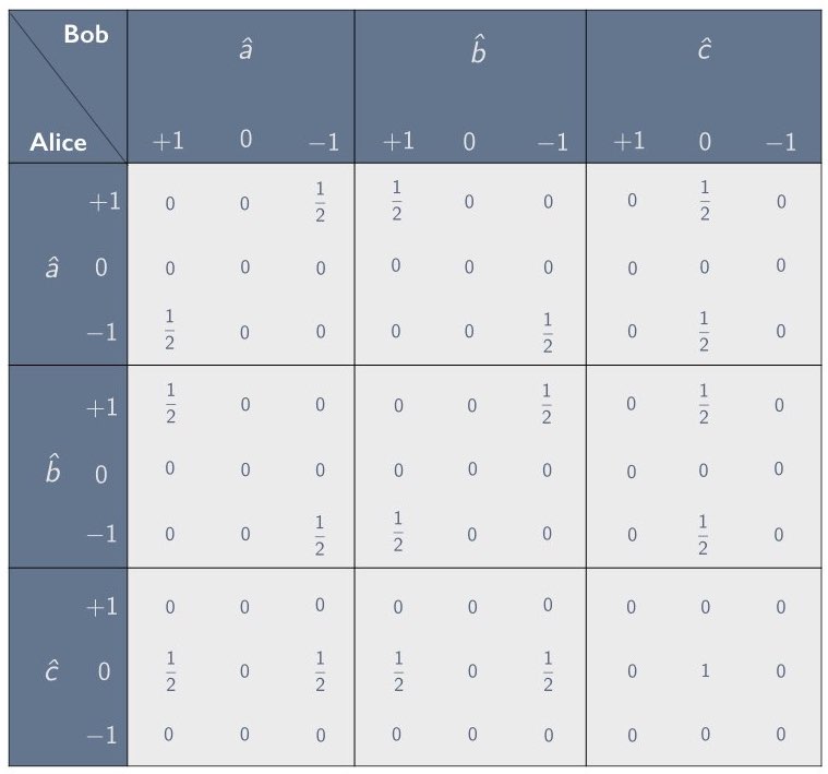
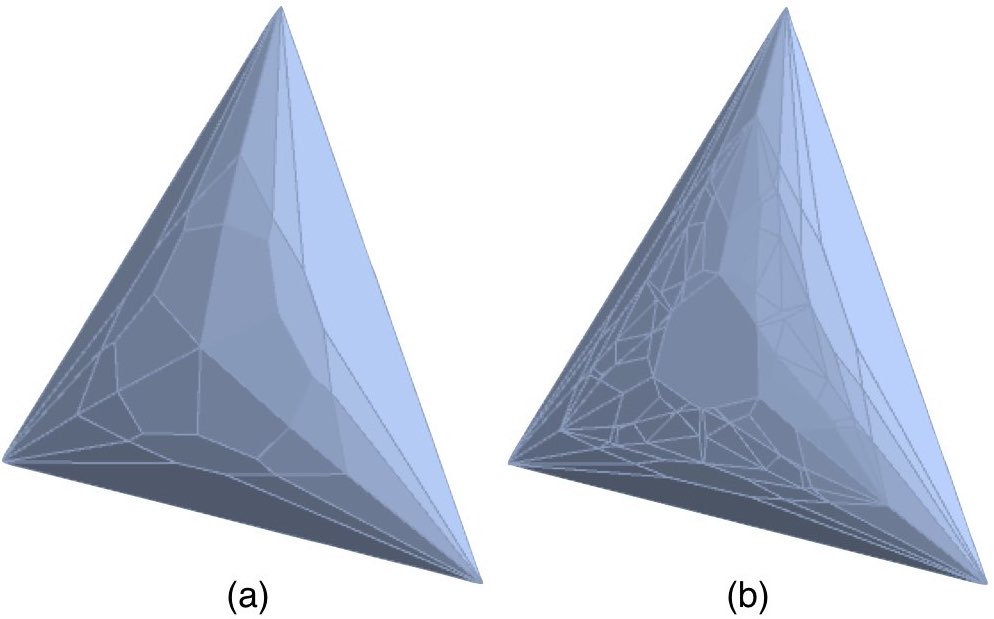
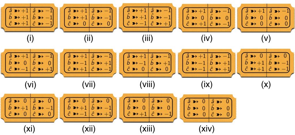
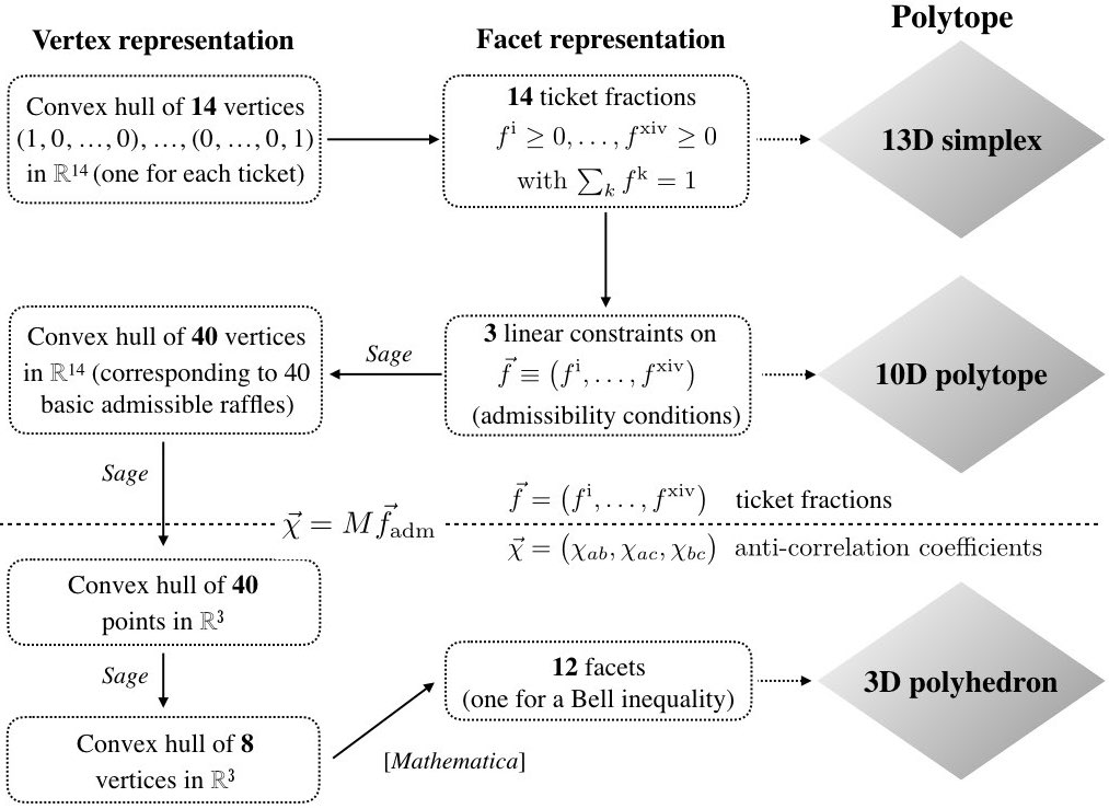
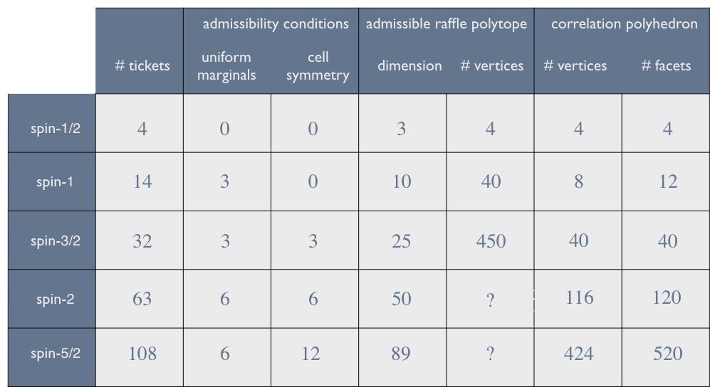
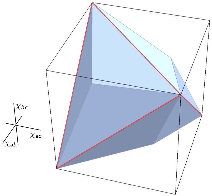
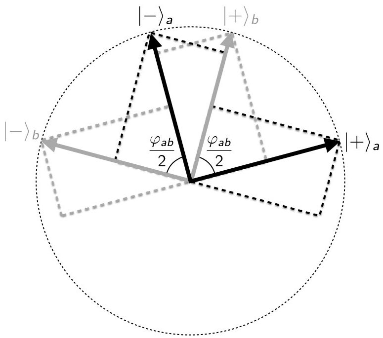
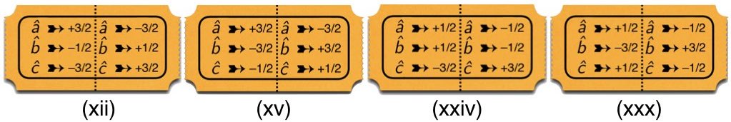
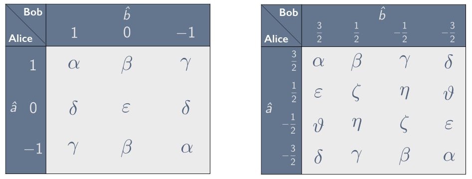
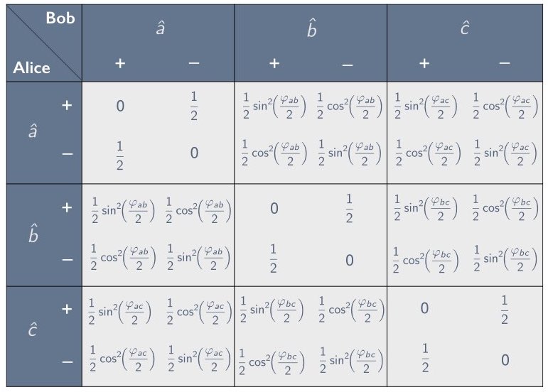
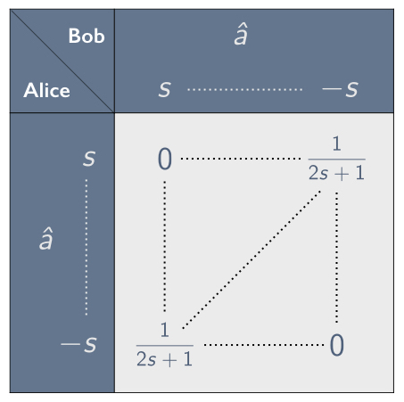
A Note of Gratitude
The copyright of this content belongs to the respective researchers. We deeply appreciate their hard work and contribution to the advancement of human civilization.-
These are identical to the inequalities given in Eqs. ([Mermin inequality CHSH-like (i)]–[Mermin inequality CHSH-like (iv)]) of Section 2.4. ↩︎
-
This equation is identical to Eq. [QM14] from Section 6.1. ↩︎
-
We call them polyhedra rather than polytopes since they are always three-dimensional. ↩︎
-
We previously noted Pitowsky’s observation in Section 1, where we quoted him. ↩︎
-
A correlation coefficient $`\overline{\chi}_{\alpha\beta}`$ is just the negative of its corresponding anti-correlation coefficient. ↩︎
-
The following equation is identical to Eq. [inf the 5] of Section 6.2.1. ↩︎
-
This equation is identical to Eq. [inf the 1] of Section 6.2.1. ↩︎
-
For further discussion, see Section 6.2.5 and in particular the caveat contained in note [no-convergence-proof]. ↩︎
-
De Finetti distinguished between coherent degrees of belief in—and therefore probabilities associated with—verifiable as opposed to unverifiable events. This has consequences for his theory of probability. For instance if $`A`$ and $`B`$ are verifiable but not jointly verifiable they are not subject to the inequality $`P(A) + P(B) - P(A\& B) \leq 1`$. See for further discussion. ↩︎
-
See note [Myrvold 2] in Section 6.2.2. ↩︎
-
For the views of one of us on what Einstein meant by this distinction and how it captures Einstein’s own scientific methodology, see , and . ↩︎
-
See the end of Section 5.1 for a discussion of the way that our characterization of the principle-theoretic and constructive approaches differs from other ways in which they have been characterized in the literature. ↩︎
-
For more on all of these and other related topics, see the collection of essays edited by . ↩︎
-
One of us has expressed previously in print the contention that only constructive approaches to physics can yield explanatory content . All three of us are now of the opinion that both principle-theoretic and constructive approaches can be explanatory. ↩︎
-
Ours is not a principle-theoretic interpretation on the way that we have expounded that term here. As discussed at the end of Section 5.1, our own usage of the term is intended to reflect its usage in the contemporary literature on quantum foundations. Our interpretation could, though, be seen as a principle-theoretic one in the sense in which (for instance) Bill Demopoulos uses that term. ↩︎
-
For a detailed reconstruction of Jordan’s argument, see . The ensuing debate over this reconstruction does not, as far as we can tell, affect our use of this example in the present context. ↩︎
-
For a detailed analysis of this episode, see . ↩︎
-
Cf. the opening sentence of the preface of his classic text on magnetic and electric susceptibilities quoted in note [Van Vleck] in Section 6.2.2, the book that earned him the informal title of “father of modern magnetism” . ↩︎
-
For a detailed analysis of this episode, see . ↩︎
-
In the case of special relativity, it also took some time for physicists to recognize that some puzzles had been resolved by the new kinematics. In the case of the Trouton-Noble experiment, was the first to show that the torque on a moving capacitor that the experimenters had been looking for in 1903 was nothing but an artifact of how one slices Minkowski space-time when defining the momentum and angular momentum of spatially extended systems . ↩︎
-
As we noted in Section 1, density operators were first introduced by . ↩︎
-
Gleason’s proof assumes that measurements are represented as projections and is valid for Hilbert spaces of dimension $`\geq 3`$. proves an analogous result for the more general class of positive operator valued measures (POVMs, or “effects”) which is valid for Hilbert spaces of dimension $`\geq 2`$. An extended discussion of the issue of completeness in relation to Gleason’s theorem may be found in . ↩︎
-
Bohr writes: “In the treatment of atomic problems, actual calculations are most conveniently carried out with the help of a Schrödinger state function, from which the statistical laws governing observations obtainable under specified conditions can be deduced by definite mathematical operations. It must be recognized, however, that we are here dealing with a purely symbolic procedure, the unambiguous physical interpretation of which in the last resort requires a reference to a complete experimental arrangement. Disregard of this point has sometimes led to confusion, and in particular the use of phrases like ‘disturbance of phenomena by observation’ or ‘creation of physical attributes of objects by measurements’ is hardly compatible with common language and practical definition.” ↩︎
-
Bohr writes: “While, however, in classical physics the distinction between object and measuring agencies does not entail any difference in the character of the description of the phenomena concerned, its fundamental importance in quantum theory, as we have seen, has its root in the indispensable use of classical concepts in the interpretation of all proper measurements, even though the classical theories do not suffice in accounting for the new types of regularities with which we are concerned in atomic physics.” Compare also : “the requirement of communicability of the circumstances and results of experiments implies that we can speak of well defined experiences only within the framework of ordinary concepts”. ↩︎
-
See for an investigation into the existence of ideal quantum measurements, and see for discussion of the quantum correlations that can be realized with ideal and non-ideal measurements. ↩︎
-
This paper deals with philosophy, pedagogy and polytopes. In this introduction, we will explain how these three components are connected, both to each other and to Bananaworld . Cuffaro’s main interest is in philosophy, Janssen’s in pedagogy and Janas’s in polytopes. Though all three of us made substantial contributions to all six sections of the paper, Janssen had final responsibility for Sections 1–2, Janas for Sections 3–4 and Cuffaro for Sections 5–6. ↩︎
-
The contemporary literature on quantum foundations has muddied the waters in regards to the classification of interpretations of quantum mechanics, and it is partly for this reason that we prefer to give a genealogy rather than a taxonomy of interpretations. Ours is not an epistemic interpretation of quantum mechanics in the sense compatible with the ontological models framework of . In particular it is not among our assumptions that a quantum system has, at any time, a well-defined ontic state. Actually we take one of the lessons of quantum mechanics to be that this view is untenable (see Section 5.3 below). For more on the differences between a view such as ours and the kind of epistemic interpretation explicated in , and for more on why the no-go theorem proved by places restrictions on the latter kind of epistemic interpretation but is not relevant to ours, see . ↩︎
-
One of us is working on a two-volume book on the genesis of quantum mechanics, the first of which has recently come out . ↩︎
-
David provides an example from the quantum foundations literature showing that the “big discoveries” of matrix and wave mechanics are not mutually exclusive. He argues that the Everett interpretation should be seen as a general new framework for physics while endorsing the view that vectors in Hilbert space represent what is real in the quantum world. Wallace and other Oxford Everettians derive the Born rule for probabilities in quantum mechanics from decision-theoretic considerations instead of taking it to be given by the Hilbert space formalism the way von Neumann showed one could (see below). For Berlin Everettians (i.e., at least some of the Christoph Lehners in their multiverse) state vectors are both ontic and epistemic. They help themselves to the Born rule à la von Neumann but also use state vectors to represent physical reality (Christoph Lehner, private communication). ↩︎
-
For historical analysis of these developments, focusing on Jordan and von Neumann, see and, for a summary aimed at a broader audience, . ↩︎
-
The video of their talk can still be watched at <users.ox.ac.uk/~everett/videobub.htm> ↩︎
-
See, e.g., the review in Physics World by Minnesota physicist Jim , well-known for his use of comic books to explain physics , and the review in Physics Today by philosopher of quantum mechanics Richard . ↩︎
-
In an essay review of , and , gives a concise characterization of his views and places them explicitly in the lineage of Heisenberg sketched above. ↩︎
-
We dedicate our paper to Bill and Itamar. See for a moving obituary of Itamar. ↩︎
-
See for an enlightening discussion of the debate over whether special relativity is best understood kinematically or dynamically. ↩︎
-
What complicates matters here is that the distinction between kinematics and dynamics tends to get conflated with the distinction between constructive and principle theories . ↩︎
-
Everettians face the same issue as part of the task of explaining how the seemingly classical (Boolean) world we find ourselves in emerges from their multiverse. Bubists could piggy-back on whatever scheme the Everettians come up with to handle this issue. ↩︎
-
In Wahrscheinlichkeitstheoretischer Aufbau, von Neumann also resisted the idea that vectors in Hilbert space ultimately represent (our knowledge of) physical reality. He wrote: “our knowledge of a system $`\mathfrak{S}'`$, i.e., of the structure of a statistical ensemble $`\{ \mathfrak{S}'_1, \mathfrak{S}'_2,`$ $`\ldots \}`$, is never described by the specification of a state—or even by the corresponding $`\varphi`$ [i.e., the vector $`| \varphi \rangle`$]; but usually by the result of measurements performed on the system” . He thus wanted to represent “our knowledge of a system” by the values of a set of observables corresponding to a complete set of commuting operators . ↩︎
-
Paraphrasing what E. M. once said about Virginia Woolf (“[S]he pushed the light of the English language a little further against the darkness”), one might say that quantum mechanics pushes physics right up to the point where total randomness takes over. ↩︎
-
We realize that it is easier to swallow this “totally random” response for the observables considered in this paper (where the spin of some particle can be up or down or a banana can taste yummy or nasty) than for others, such as, notably, position (where a particle can be here or on the other side of the universe). ↩︎
-
See Section 5.5 for careful discussion of how our profound measurement problem differs from their “small” one. ↩︎
-
See Figure 3 for the correlation array for a PR box. Figure 9 shows that it is impossible to design tickets for a raffle that could simulate the correlations generated by a PR box. ↩︎
-
We took the within/without terminology from the chorus of “Quinn the Eskimo,” a song from Bob Dylan’s 1967 Basement Tapes: “Come all without, come all within. You’ll not see nothing like the mighty Quinn.” Could “the mighty Quinn” be an oblique but prescient reference to a quantum computer? ↩︎
-
See for a concise account, written for a general audience and based on interviews with some of the principals, of how the CHSH inequality was formulated and experimentally tested. ↩︎
-
also cites , his contribution to a Festschrift for Bub, as well as . ↩︎
-
Betraying his information-theoretic leanings, occasionally refers to inputs and outputs (both taking on the values 0 and 1) rather than peelings and tastes (see, e.g., p. 51, Figure 3.1). ↩︎
-
Bub’s illustrator, his daughter Tanya, has the Cheshire Cat (starring as Clio) peel the third GHZ banana . ↩︎
-
In Mermin’s (1981, p. 86) example, there is a perfect (positive) correlation in runs in which the two parties use the same setting and an imperfect anti-correlation in runs in which they use different settings (see also Mermin, 1988, pp. 135–136). To get Mermin’s original example, we should have used our pairs of bananas to represent entangled pairs of photons and let “peel and taste bananas using different peeling directions” stand for “measure the polarization of these photons along different axes”. We got our variation on Mermin’s example by having pairs of bananas represent pairs of spin-$`\frac12`$ particles entangled in the singlet state and letting “peel and taste bananas using different peeling directions” stand for “measure spin components of these particles along different axes” (see Section 6.1). ↩︎
-
Part of what makes it interesting to contemplate entangled quoins or bananas is that we are free to choose when to toss or taste them whereas with entangled photons or spin-$`\frac12`$ particles we have no choice but to measure their polarization or spin as soon as they arrive at our detectors. ↩︎
-
It does not matter in what order Alice and Bob peel their bananas. The correlations in the correlation array in Figure 3 represent constraints on possible combinations of outcomes found by Alice and Bob, not some mechanism through which the outcome of one peeling would cause the outcome of the other. ↩︎
-
In Bananaworld, Bub leaves it to the reader to find examples of correlation arrays that violate the non-signaling condition. Below are the entries for two such correlation arrays:
MATH(a) \quad \begin{array}{cccc} 1 & 0 & 0 & 0 \; \\ 0 & 0 & 0 & 1 \; \\ 0 & 0 & 1 & 0 \; \\ 0 & 1 & 0 & 0, \end{array} \quad \quad \quad (b) \quad \begin{array}{cccc} \boldsymbol{6/10} & 1/10 & 2/10 & 1/10 \; \\ 1/10 & 2/10 & 1/10 & \boldsymbol{6/10} \; \\ 2/10 & 1/10 & \boldsymbol{6/10} & 1/10 \; \\ 1/10 & \boldsymbol{6/10} & 1/10 & 2/10. \end{array}Click to expand and view moreIf there were a system producing the distant correlations in (a), be it pairs of bananas or pairs of coins, one pair would suffice for Alice and Bob to transmit one bit of information to the other party instantaneously; if there were a system producing the distant correlations in (b), several pairs would be needed to do so with some fidelity. The latter system can be thought of as a noisy version of the former. ↩︎
-
In Section 5 we will see that there is an extra bonus to discussing classical theory in terms of such raffles. It makes for a natural comparison between local hidden-variable theories and John von Neumann’s (1927b) formulation of quantum theory in terms of statistical ensembles characterized by density operators on Hilbert space. Single-ticket raffles, i.e., raffles with baskets of tickets that are all the same, are the classical analogues of pure states in quantum mechanics; mixed raffles, i.e., raffles with baskets with different tickets, are the analogues of mixed states. By using the imagery of baskets with different mixes of tickets, we admittedly sweep a mathematical subtlety under the rug: the fractions of different types of tickets in a basket will always be rational numbers. To simulate the quantum correlations we are interested in, however, we need to allow fractions that are real numbers. In Section 6.2.6 we will introduce a different mechanism for selecting tickets that gets around this problem (see Figure [wheelsoffortune]). From a practical point of view, the restriction to rationals is harmless, since the rationals are dense in the reals. ↩︎
-
Essentially the same argument can already be found in . ↩︎
-
For a formal proof of this intuitively plausible result, see Section 6.2.6. ↩︎
-
For a drawing of their apparatus see . This drawing is based on a photograph that can be found, for instance, in . For a schematic drawing of the apparatus, see . ↩︎
-
David Kaiser alerted us to a paper written by 20 authors (with Kaiser, Alan Guth and Anton Zeilinger listed in 17th, 18th and 20th place, respectively) about one of the latest initiatives in this ongoing effort . ↩︎
-
We still do not need the stronger assumption that these decisions are made only after they receive their banana, their spin-$`\frac12`$ particle, or their ticket stub. ↩︎
-
Cf. , who argues that the Everett interpretation provides a general “recipe” for interpreting quantum theory (see also note 30 in Section 1). ↩︎
-
Bohr writes: “the proper rôle of the indeterminacy relations consists in assuring quantitatively the logical compatibility of apparently contradictory laws which appear when we use two different experimental arrangements, of which only one permits an unambiguous use of the concept of position, while only the other permits the application of the concept of momentum.” ↩︎