Saddlepoint Approximations for Spatial Panel Data Models with Fixed Effects and Time-Varying Covariates

First-order asymptotics

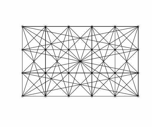
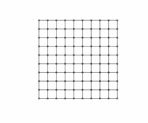
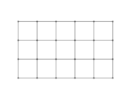
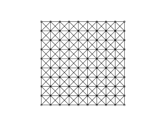
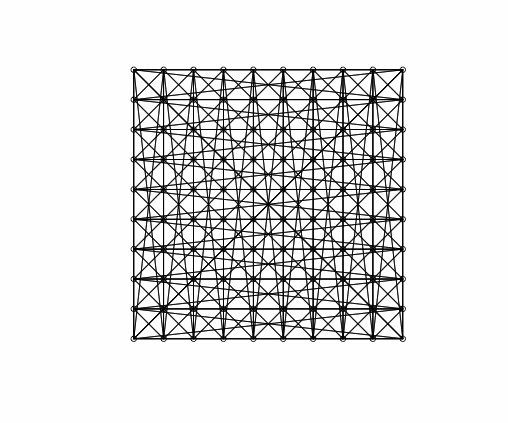
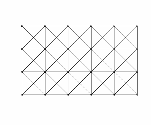
As it is customary in the statistical/econometric software, we consider three different spatial weight matrices: Rook matrix, Queen matrix, and Queen matrix with torus. In Figure 1, we display the geometry of $`Y_{nt}`$ as implied by each considered spatial matrix for $`n=100`$: the plots highlight that different matrices imply different spatial relations. For instance, we see that the Rook matrix implies fewer links than the Queen matrix. Indeed, the Rook criterion defines neighbours by the existence of a common edge between two spatial units, whilst the Queen criterion is less rigid and defines neighbours as spatial units sharing an edge or a vertex. Besides, we may interpret $`\{Y_{nt}\}`$ as a $`n`$-dimensional random field on the network graph which describes the known underlying spatial structure. Then, $`W_n`$ represents the weighted adjacency matrix (in the spatial econometrics literature, $`W_n`$ is called contiguity matrix). In Figure 1, we display the geometry of a random field on a regular lattice (undirected graph).

Rook Queen Queen torus

style="width:32.5%;height:25.0%" /> style="width:32.5%;height:25.0%" /> style="width:32.5%;height:25.0%" />

We complement the motivating example of our research illustrating the low accuracy of the routinely applied first-order asymptotics in the setting of the spatial autoregressive process of order one, henceforth SAR(1):

\begin{equation}
\begin{aligned}
Y\nt &=& \lambda_0 W_n Y\nt + c_{n0} + V\nt,   \quad {\text{for}} \quad t=1,2, 
\end{aligned}
\label{Eq: RR}
\end{equation}

where $`V\nt =(v_{1t},v_{2t},..,v\nt)'`$ are $`n \times 1`$ vectors, and $`v_{it}\sim \mathcal{N}(0,1)`$, i.i.d. across $`i`$ and $`t`$. The model is a special case of the general model in (2.1), the spatial autoregressive process with spatial autoregressive error (SARAR) of . Since $`c_{n0}`$ creates an incidental parameter issue, we eliminate it by the standard differentiation procedure. Given that we have only two periods, the transformed (differentiated) model is formally equivalent to the cross-sectional SAR(1) model, in which $`c_{n0} \equiv 0`$, a priori; see for a related discussion.

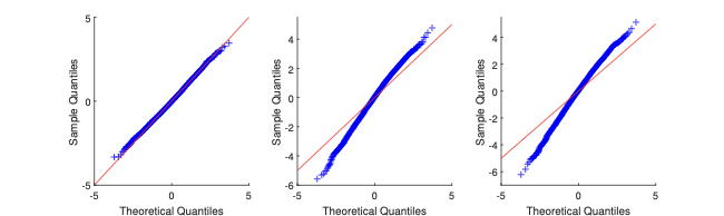
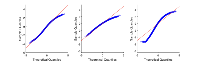
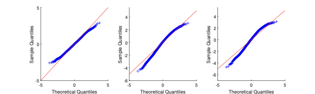
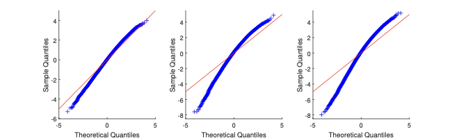
In the MC exercise, we set $`\lambda_0 = 0.2`$, and we estimate it through Gaussian likelihood maximisation. The resulting $`M`$-estimator (the maximum likelihood estimator) is consistent and asymptotically normal; see §4.1. We consider the same types of $`W_n`$ as in the motivating example of §2. In Figure 2, we display the MC results. Via QQ-plot, we compare the distribution of $`\hat\lambda`$ to the Gaussian asymptotic distribution (as implied by the first-order asymptotic theory).

Rook Queen Queen torus

90 n = 24 style="width:90.0%;height:20.0%" />

90 n = 100 style="width:90.0%;height:20.0%" />

The plots show that, for both sample sizes $`n=24`$ and $`=100`$, the Gaussian approximation can be either too thin or too thick in the tails with respect to the “exact” distribution (as obtained via simulation). The more complex is the geometry of $`W_n`$ (e.g., $`W_n`$ is Queen), the more pronounced are the departures from the Gaussian approximation.

Assumption D(iv) and its relation to the spatial weights

We can obtain $`M_{i,T}(\psi,P_{\theta _{0}})`$ from (4.4) on a SAR(1) model as in ([Eq: RR]),

M_{i,T}(\psi,P_{\theta _{0}})=(T-1)( \tilde{g}_{ii}+g_{ii}),

where $`\tilde{g}_{ii}`$ and $`g_{ii}`$ are the $`i_{th}`$ element of the diagonals of $`G_nG'_n`$ and $`G^2_n(\lambda_0)`$, respectively. Note that $`S_n(\lambda_0)=I_n-\lambda_0 W_n`$ and $`G_n(\lambda_0) = W_nS_n^{-1}(\lambda_0)`$.

To check Assumption D(iv): $`\vert\vert M_{i,T}(\psi,P_{\theta _{0}})-M_{j,T}(\psi,P_{\theta _{0}})\vert\vert=O(n^{-1})`$, first let us find the expression for the difference between $`M_{i,T}(\psi,P_{\theta _{0}})`$ and $`M_{j,T}(\psi,P_{\theta _{0}})`$,

\begin{eqnarray}
M_{i,T}(\psi,P_{\theta _{0}})-M_{j,T}(\psi,P_{\theta _{0}}) &=& (T-1)\l[\l(\tilde{g}_{ii}-\tilde{g}_{jj}\r)+\l(g_{ii}-g_{jj}\r)\r] ,
\end{eqnarray}

where $`\tilde{g}_{ii}`$ and $`\tilde{g}_{ii}`$ are $`i_{th}`$ and $`j_{th}`$ elements of the diagonal of $`G_nG'_n`$. $`g_{ii}`$ snd $`g_{jj}`$ the $`i_{th}`$ and $`j_{th}`$ elements of the diagonal of $`G^2_n(\lambda_0)`$. Then, we rewrite the expression of $`G_n^2(\lambda_0)`$ to check its diagonal:

\begin{eqnarray}
G_n^2(\lambda_0) &=& W^2_nS_n^{-2}(\lambda_0) = W_n^2\l(I_n-\lambda_0W_n\r)^{-2} \nn \\
&=&W^2_n\l(I_n+\lambda_0W_n+\lambda_0^2W_n^2+\lambda_0^3W_n^3+\cdots\r)^2 \nn \\
&=& \sum_{k=2}^{\infty}a_kW_n^k,
\end{eqnarray}

where $`a_k`$ is the coefficient of $`W_n^k`$. By comparing the entries of diagonals of $`W_n^k`$, we can make an assumption on the differences between any two entries of the diagonal of $`W_n^k`$ that should be at most of order $`n^{-1}`$, for all integers $`k \ge 2`$, such that $`||{g}_{ii}-{g}_{jj}|| = O(n^{-1})`$, for any $`1\le i`$, $`j \le n`$ and $`i\ne j`$.

We do the same for $`G_nG'_n`$:

\begin{eqnarray}
G_nG'_n &=& W_nS_n^{-1}(\lambda_0) \l(W_nS_n^{-1}(\lambda_0) \r)'= W_n\l(I_n-\lambda_0W_n\r)^{-1}\l(W_n\l(I_n-\lambda_0W_n\r)^{-1}\r)' \nn \\
&=&W_n\l(I_n+\lambda_0W_n+\lambda_0^2W_n^2+\lambda_0^3W_n^3+\cdots\r)\l(I_n+\lambda_0W_n+\lambda_0^2W_n^2+\lambda_0^3W_n^3+\cdots\r)'W'_n\nn \\
&=& \sum_{k_1=1}^{\infty}\sum_{k_2=1}^{\infty}a_{k_1k_2} W_n^{k_1}\l(W_n^{k_2}\r)',
\end{eqnarray}

where $`a_{k_1k_2}`$ is the coefficient of $`W_n^{k_1}\l(W_n^{k_2}\r)'`$. Then, we can make a second assumption on the differences between any two entries of the diagonal of $`W_n^{k_1}\l(W_n^{k_2}\r)'`$ that should be at most of order $`n^{-1}`$, for all positive integers $`k_1`$ and $`k_2`$, such that $`||\tilde{g}_{ii}-\tilde{g}_{jj}|| = O(n^{-1})`$, for any for any $`1\le i`$, $`j \le n`$ and $`i\ne j`$. From those two assumptions on the behaviour of diagonal entries, we notice that $`W_n`$ plays a leading role.

To exemplify those two conditions, we consider numerical examples for different choices of $`W_n`$. The sample size $`n`$ is $`24`$ with the benchmark $`1/n = 1/24 = 0.041`$. When $`W_n`$ is Rook, the elements of $`W_n`$ are $`\{1/2,1/3,1/4,0\}`$. On top of that, we can find the differences between the entries of the diagonals of $`W_n^k`$ and $`W_n^{k_1}\l(W_n^{k_2}\r)'`$ are small. For instance, the entries of the diagonal of $`W_n^2`$ are $`\{0.27,0.29,0.31,0.33,0.36\}`$. The elements of diagonal of $`W_n^3`$ are all $`0`$. For $`W_n^2(W_n^2)'`$, the entries of its diagonal are {0.17,0.21,0.22,0.37}. We can obtain a similar result for Queen weight matrix. For example, the largest difference between diagonal entries of $`W_n^2`$ is $`0.044`$. When $`W_n`$ is Queen with torus, $`W_n`$ is a symmetric matrix and its elements are $`0`$ or $`1/8`$. The entries of the diagonals of $`W_n^k`$ and $`W_n^{k_1}\l(W_n^{k_2}\r)'`$ are always identical to each other. Thus, the differences are always $`0`$. Since the entries of $`W_n`$ are all positive and less than $`1`$, when the exponent becomes larger, all the values of the powers of $`W_n`$ and $`W'_n`$ will go close to $`0.00`$. Thus, large powers of $`W_n`$ definitely satisfy the two assumptions.

First-order asymptotics vs saddlepoint approximation

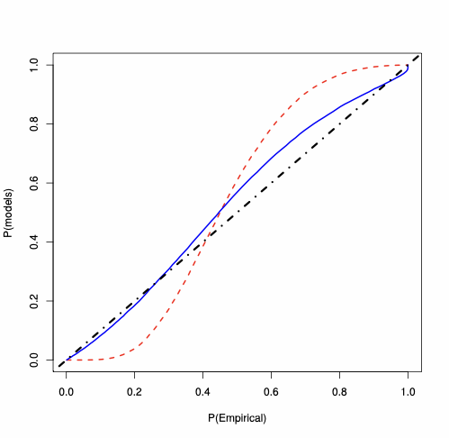
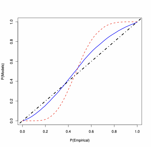
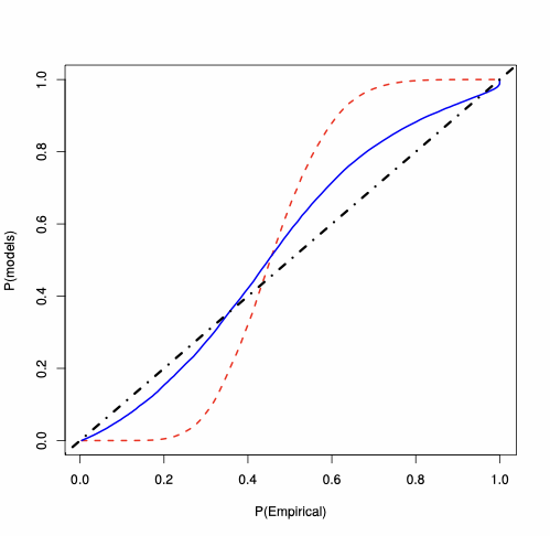
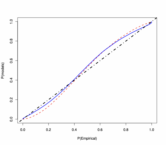
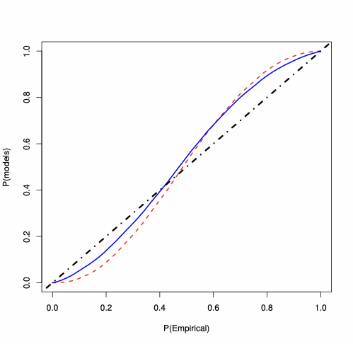
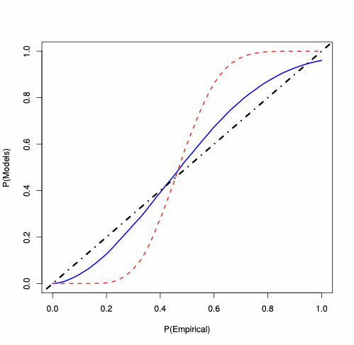
For the SAR(1) model, we analyse the behaviour of the MLE of $`\lambda_0`$, whose PP-plots are available in Figure 3. For each type of $`W_n`$, for $`n=100`$, the plots show that the saddlepoint approximation is closer to the “exact” probability than the first-order asymptotics approximation. For $`W_n`$ Rook, the saddlepoint approximation improves on the routinely-applied first-order asymptotics. In Figure 3, the accuracy gains are evident also for $`W_n`$ Queen and Queen with torus, where the first-order asymptotic theory displays large errors essentially over the whole support (specially in the tails). On the contrary, the saddlepoint approximation is close to the 45-degree line.

Rook	Queen	Queen torus
90 n = 100 style="width:30.0%;height:26.5%" />	style="width:30.0%;height:26.5%" />	style="width:30.0%;height:26.5%" />

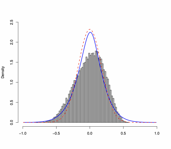
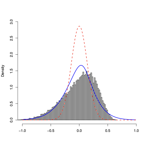
Density plots show the same information as PP-plots displayed in Figure 3 (of the paper) and Figure 3 (in this Appendix), but provide a better visualization of the behavior of the considered approximations. Thus, we compute the Gaussian density implied by the asymptotic theory, and we compare it to our saddlepoint density approximation. In Figure 4, we plot the histogram of the “exact” estimator density (as obtained using 25,000 Monte Carlo runs) to which we superpose both the Gaussian and the saddlepoint density approximation. $`W_n`$ are Rook and Queen. The plots illustrate that the saddlepoint technique provides an approximation to the true density which is more accurate than the one obtained using the first-order asymptotics.

Rook & n = 24	Queen & n = 24
style="width:40.0%;height:25.0%" />	style="width:40.0%;height:25.0%" />

Saddlepoint approximation vs Edgeworth expansion

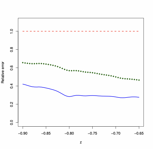
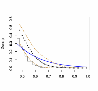
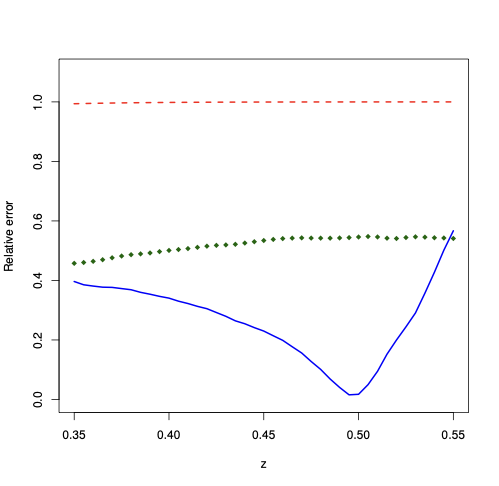
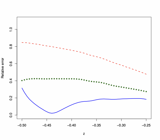
The Edgeworth expansion derived in Proposition 3 represents the natural alternative to the saddlepoint approximation since it is fully analytic. Thus, we compare the performance of the two approximations, looking at their relative error for the approximation of the tail area probability. We keep the same Monte Carlo design as in Section 6.1, namely $`n=24`$, and we consider different values of $`z`$, as in (4.15). Figure 5 displays the absolute value of the relative error, i.e., $`|\text{approximation}/ \text{exact} -1 |`$, when $`W_n`$ is Rook, Queen, and Queen torus. The plots illustrate that the relative error yielded by the saddlepoint approximation is smaller (down to ten times smaller in the case of Rook and Queen Torus) than the relative error entailed by the first-order asymptotic approximation (which is always about 100%). The Edgeworth expansion entails a relative error which is typically higher than the one entailed by the saddlepoint approximation—the expansion can even become negative in some parts of the support, with relative error above 100%.

Rook Left	Queen Left	Queen Torus Right
style="width:30.0%;height:25.0%" />	style="width:30.0%;height:25.0%" />	style="width:30.0%;height:25.0%" />

Saddlepoint vs parametric bootstrap

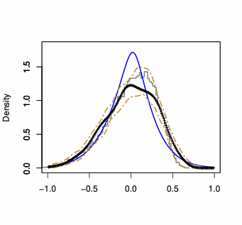
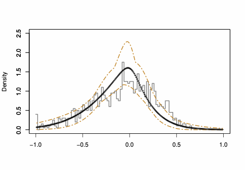
The parametric bootstrap represents a (computer-based) competitor, commonly applied in statistics and econometrics. To compare our saddlepoint approximation to the one obtained by bootstrap, we consider different numbers of bootstrap repetitions, labeled as $`B`$: we use $`B=499`$ and $`B=999`$. For space constraints, in Figure 6, we display the results for $`B=499`$ (similar plots are available for $`B=999`$) showing the functional boxplots (as obtained iterating the procedure 100 times) of the bootstrap approximated density, for sample size $`n =24`$ and for $`W_n`$ is Queen.

style="width:48.5%;height:35.0%" />

style="width:48.5%;height:35.0%" />

To visualize the variability entailed by the bootstrap, we display the first and third quartile curves (two-dash lines) and the median functional curve (dotted line with crosses); for details about functional boxplots, we refer to and to R routine fbplot. We notice that, while the bootstrap median functional curve (representing a typical bootstrap density approximation) is close to the actual density (as represented by the histogram), the range between the quartile curves illustrates that the bootstrap approximation has a variability. Clearly, the variability depends on $`B`$: the larger is $`B`$, the smaller is the variability. However, larger values of $`B`$ entail bigger computational costs: when $`B=499`$, the bootstrap is almost as fast as the saddlepoint density approximation (computation time about 7 minutes, on a 2.3 GHz Intel Core i5 processor), but for $`B=999`$, it is three times slower. We refer to for comments on the computational burden of the parametric bootstrap and on the possibility to use saddlepoint approximations to speed up the computation. For $`B=499`$ and zooming on the tails, we notice that in the right tail and in the center of the density, the bootstrap yields an approximation (slightly) more accurate than the saddlepoint method, but the saddlepoint approximation is either inside or extremely close to the bootstrap quartile curves (see right panel of Figure 6). In the left tail, the saddlepoint density approximation is closer to the true density than the bootstrap typical functional curve or $`\lambda \leq -0.85`$. Thus, overall, we cannot conclude that the bootstrap dominates uniformly (in terms of accuracy improvements over the whole domain) the saddlepoint approximation. Even if we are ready to accept a larger computational cost, the accuracy gains yielded by the bootstrap are yet not fully clear: also for $`B=999`$, the bootstrap does not dominate uniformly the saddlepoint approximation. Finally, for $`B = 49`$, the bootstrap is about eight times faster than the saddlepoint approximation, but this gain in speed comes with a large cost in terms of accuracy. As an illustration, for $`\hat\lambda-\lambda_0=-0.8`$ (left tail), the true density is $`0.074`$, the saddlepoint density approximation is $`0.061`$, while the bootstrap median value is $`0.040`$, with a wide spread between the first and the third quartile, being $`0.009`$ and $`0.108`$ respectively.

Saddlepoint test for composite hypotheses: plug-in approach

Our saddlepoint density and/or tail approximations are helpful for testing simple hypotheses about $`\theta_0`$; see §6.1 of the paper. Another interesting case suggested by the Associate Editor and an anonymous referee that has a strong practical relevance is related to testing a composite null hypothesis. It is a problem which is different from the one considered so far in the paper, because it raises the issue of dealing with nuisance parameters.

To tackle this problem, several possibilities are available. For instance, we may fix the nuisance parameters at the MLE estimates. Alternatively, we may consider to use the (re-centered) profile estimators, as suggested, e.g., in and . Combined with the saddlepoint density in (4.13), these techniques yield a ready solution to the nuisance parameter problem. In our numerical experience, these solutions may preserve reasonable accuracy in some cases.

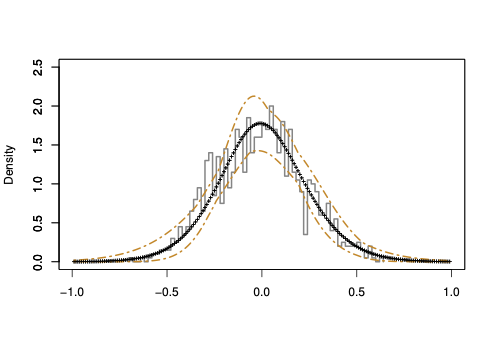
To illustrate this aspect, we consider a numerical exercise about SAR(1) model, in which we set the nuisance parameter equal to the MLE estimate. Specifically, we consider a SAR(1) with parameter $`\theta=(\lambda,\sigma^2)'`$ and our goal is to test $`\mathcal{H}_0: \lambda=\lambda_0 = 0`$ versus $`\mathcal{H}_1: \lambda > 0`$, while leaving $`\sigma^2`$ unspecified. To study the performance of the saddlepoint density approximation for the sampling distribution of $`\hat\lambda`$, we perform a MC study, in which we set $`n=24`$, $`T=2`$, and $`\sigma_0^2=1`$. For each simulated (panel data) sample, we estimate the model parameter via MLE and get $`\hat\theta = (\hat\lambda,\hat\sigma^2)'`$. Then, we compute the saddlepoint density in (4.13) using $`\hat\sigma^2`$ in lieu of $`\sigma^2_0`$: for each sample, we have a saddlepoint density approximation. We repeat this procedure 100 times, for $`W_n`$ Rook and Queen, so we obtain 100 saddlepoint density approximations for each $`W_n`$ type. In Figure 7, we display functional boxplots of the resulting saddlepoint density approximation for the MLE $`\hat\lambda`$. To have a graphical idea of the saddlepoint approximation accuracy, on the same plot we superpose the histogram of $`\hat\lambda`$, which represents the sampling distribution of the estimated parameter. Even a quick inspection of the right and left plots suggests that the resulting saddlepoint density approximation preserves (typically) a good performance. Indeed, we find that the median functional curve (dotted line with crosses, which we consider as the typical saddlepoint density approximation) is close to the histogram and it gives a good performance in the tails, for both $`W_n`$ Rook and Queen. The range between the first and third quartile curves (two-dash lines) illustrates the variability of the saddlepoint approximation. When $`W_n`$ is Queen, even though there is a departure from the median curve from the histogram over the x-axis intervals $`(-0.75,0)`$ and $`(0.25,0.5)`$, the histogram is inside the functional confidence interval expressed by the first and third curves. Thus, we conclude that computing the $`p`$-value for testing $`\mathcal{H}_0`$ using $`\hat\sigma^2`$ in the expression of the saddlepoint density approximation seems to preserve accuracy in this SAR(1) model, even for such a small sample.

Rook & n = 24	Queen & n = 24
style="width:47.5%;height:35.0%" />	style="width:47.5%;height:35.0%" />

Component-wise calculation of $`- \mathbb{E} \left( \frac{1}{m} \frac{\partial^2 \ell_{n,T}(\theta_0)}{\partial \theta \partial \theta'} \right)`$

From the model setting, we have $`V_{nt} = (V_{1t},V_{2t},\cdots V_{nt})`$ and $`V_{it}`$ is i.i.d. across i and t with zero mean and variance $`\sigma_0^2`$. So $`\mathbb{E}(V_{nt}) = 0_{n \times 1}`$, $`Var(V_{nt})=\sigma_0^2I_n`$. Knowing that $`\tVn = V_{nt}-\sum_{t=1}^{T}V_{nt}/T`$,
$`\mathbb{E}(\tVn)=0_{n \times 1}`$, $`Var(\tVn)= Var((1-1/T)V_{nt}+1/T \sum_{j=1,j\neq t}^{T} V_{nj})=\frac{T-1}{T}\sigma_0^2 I_n`$.
$`\tVn=\Rn[S_n(\lambda) \tYn-\tXn \beta]`$, so $`\mathbb{E}(\tYn)= S_n^{-1}(\lambda)\tXn \beta`$.
Some other notations: $`\ddot{X}_{nt} = R_n\tXn, H_n=M_n R_n^{-1}, G_n=W_n S_n^{-1},\ddot{G}_n=R_n G_n R_n^{-1}`$.

• = _t=1^T_nt^’_nt

  MATH

  Collapse Copy

  \begin{eqnarray}
  \mathbb{E}\left[ \frac{1}{m\sigma_0^{2}} \sum_t (R_n(\rho_0) W_n \tYn)'(R_n(\rho_0) \tXn) \right] &=& \frac{1}{m\sigma_0^{2}}\sum_t \left(R_n(\rho_0) W_n E(\tYn)\right)'(R_n(\rho_0) \tXn) \nonumber \\   
  &=& \frac{1}{m\sigma_0^{2}}\sum_t (R_n(\rho_0) \underbrace{W_n S_n^{-1}}_{G_n}\tXn\beta_0)'\ddot{X}_{nt} \nonumber \\
  &=& \frac{1}{m\sigma_0^{2}} \sum_t (R_n(\rho_0) G_nR_n^{-1}R_n\tXn\beta_0)'\ddot{X}_{nt} \nonumber \\ 
  &=& \frac{1}{m\sigma_0^{2}}\sum_t (\ddot{G}_n(\lambda_0)\ddot{X}_{nt}\beta_0)'\ddot{X}_{nt}
  \end{eqnarray}

  Click to expand and view more
  MATH

  Collapse Copy

  \begin{eqnarray}
  &&\mathbb{E}\left[\frac{1}{m\sigma_0^{2}} \sum_t \left\{(H_n(\rho_0) \tilde{V}_{nt}(\xi_0))'(R_n(\lambda_0) \tXn) + \tilde{V}_{nt}^{'}(\xi_0) M_n \tXn\right\}\right] \nonumber \\
  &&= \frac{1}{m\sigma_0^{2}} \sum_t \left\{(H_n(\rho_0) \mathbb{E}\left[\tilde{V}_{nt}(\xi_0)\right])'(R_n(\lambda_0) \tXn) + \mathbb{E}\left[\tilde{V}_{nt}^{'}(\xi_0)\right] M_n \tXn\right\}=0_{1 \times k} \nn \\
  \end{eqnarray}

  Click to expand and view more
  MATH

  Collapse Copy

  \begin{eqnarray}
  \mathbb{E}\left[\frac{1}{m\sigma_0^{4}} \sum_t \tilde{V}_{nt}^{'}(\xi_0)R_n(\lambda_0)\tXn \right] &=& \frac{1}{m\sigma_0^{4}} \sum_t \mathbb{E}\left[\tilde{V}_{nt}^{'}(\xi_0)\right] R_n(\lambda_0)\tXn =0_{1 \times k} \nn \\
  \end{eqnarray}

  Click to expand and view more

  So we prove the first column of $`\Sigma_{0,n,T}`$, that is:

  MATH

  Collapse Copy

  \begin{eqnarray*}
  \frac{1}{m\sigma_0^2} \left( \begin{array}{c}    \sum_{t}\ddot{X}_{nt}^{'}\ddot{X}_{nt}    \\
                                                  \sum_t (\ddot{G}_n(\lambda_0)\ddot{X}_{nt}\beta_0)'\ddot{X}_{nt} \\
                                                  0_{1  \times k}  \\    
                                                  0_{1  \times k}    
   \end{array}\right)
  \end{eqnarray*}

  Click to expand and view more
• MATH

  Collapse Copy

  \begin{eqnarray}
  & &\mathbb{E}\left[ \frac{1}{m\sigma_0^{2}} \sum_t \left(R_n(\rho_0) W_n \tYn)'(R_n(\rho_0)W_n \tYn\right) + \frac{T-1}{m} \text{tr}(G_n^2(\lambda_0))\right] \nonumber \\
  & &= \mathbb{E}\left[ \frac{1}{m\sigma_0^{2}} \sum_t \left(R_n W_n S_n^{-1}(R_n^{-1}\tilde{V}_{nt}+\tXn \beta_0)\right)' \left(R_nW_n S_n^{-1}(R_n^{-1}\tilde{V}_{nt}+\tXn \beta_0)\right)\right] \nn \\
  && + \frac{1}{n} \text{tr}(G_n^2(\lambda_0)) \nonumber\\
  & &=\mathbb{E}\left[ \left(\frac{1}{m\sigma_0^{2}} \sum_t \left(\ddot{G}_n\tilde{V}_{nt}(\xi_0)+\ddot{G}_n\ddot{X}_{nt}\beta_0 \right)' \left(\ddot{G}_n\tilde{V}_{nt}(\xi_0)+\ddot{G}_n\ddot{X}_{nt}\beta_0\right)\right)\right]+\frac{1}{n} \text{tr}(G_n^2(\lambda_0)) \nonumber\\
  & &=\mathbb{E}\left[\frac{1}{m\sigma_0^{2}}\sum_t \left(\ddot{G}_n(\lambda_0)\tilde{V}_{nt}(\xi_0)\right)'\left(\ddot{G}_n(\lambda_0)\tilde{V}_{nt}(\xi_0)\right)\right]\nn \\
  &&+\frac{1}{m\sigma_0^{2}} \sum_t\left(\ddot{G}_n(\lambda_0)\ddot{X}_{nt}\beta_0\right)'\left(\ddot{G}_n(\lambda_0)\ddot{X}_{nt}\beta_0\right) \nonumber \\
  & &+\frac{1}{m\sigma_0^{2}}\sum_t \left(\ddot{G}_n(\lambda_0)\ddot{X}_{nt}\beta_0\right)'\ddot{G}_n(\lambda_0)\underbrace{\mathbb{E}\left[\tilde{V}_{nt}(\xi_0)\right]}_{0_{n \times 1}}+\frac{1}{n} \text{tr}(G_n^2(\lambda_0)) \nonumber \\
  & &=\frac{1}{n} \text{tr}(\ddot{G}_n^{'}(\lambda_0)\ddot{G}_n(\lambda_0))+\frac{1}{n} \text{tr}(R_n^{-1}(\rho_0)R_n(\rho_0)G_n^2(\lambda_0))
  \nn \\&&+\frac{1}{m\sigma_0^{2}} \sum_t\left(\ddot{G}_n(\lambda_0)\ddot{X}_{nt}\beta_0\right)'\left(\ddot{G}_n(\lambda_0)\ddot{X}_{nt}\beta_0\right) \nonumber \\ 
  & &=\frac{1}{n} \text{tr}\left(\ddot{G}_n^{'}(\lambda_0)\ddot{G}_n(\lambda_0)+R_n(\rho_0)G_n(\lambda_0)R_n^{-1}(\rho_0)R_n(\rho_0)G_n(\lambda_0)R_n^{-1}\right) \nonumber \\
  & &+\frac{1}{m\sigma_0^{2}} \sum_t\left(\ddot{G}_n(\lambda_0)\ddot{X}_{nt}\beta_0\right)'\left(\ddot{G}_n(\lambda_0)\ddot{X}_{nt}\beta_0\right) \nonumber \\ 
  & &=\frac{1}{n} \text{tr}\left(\ddot{G}_n^{'}(\lambda_0)\ddot{G}_n(\lambda_0)+\ddot{G}_n(\lambda_0)\ddot{G}_n(\lambda_0)\right)+\frac{1}{m\sigma_0^{2}} \sum_t\left(\ddot{G}_n(\lambda_0)\ddot{X}_{nt}\beta_0\right)'\left(\ddot{G}_n(\lambda_0)\ddot{X}_{nt}\beta_0\right) \nonumber \\ 
  & &=\frac{1}{n} \text{tr}\left(\ddot{G}_n^{S}(\lambda_0)\ddot{G}_n(\lambda_0)\right)+\frac{1}{m\sigma_0^{2}} \sum_t\left(\ddot{G}_n(\lambda_0)\ddot{X}_{nt}\beta_0\right)'\left(\ddot{G}_n(\lambda_0)\ddot{X}_{nt}\beta_0\right)
  \end{eqnarray}

  Click to expand and view more
  MATH

  Collapse Copy

  \begin{eqnarray}
  & &\mathbb{E}\left[ \frac{1}{m \sigma_0^{2}} \sum_t (R_n(\rho_0) W_n \tYn)'(H_n(\lambda_0)  \tilde{V}_{nt}(\xi_0)) + \frac{1}{m\sigma^{2} }\sum_t  (M_n W_n \tYn)' \tilde{V}_{nt}(\xi_0) \right] \nonumber \\
  & &=  \mathbb{E}\left[ \frac{1}{m \sigma_0^{2}} \sum_t  \left(R_n(\rho_0) W_n S_n^{-1}(\lambda_0)(R_n^{-1}(\rho_0)\tilde{V}_{nt}(\xi_0)+\tXn \beta_0)\right)'(H_n(\lambda_0)  \tilde{V}_{nt}(\xi_0)) \right] \nonumber\\
  & &+ \mathbb{E}\left [  \frac{1}{m \sigma_0^{2}} \sum_t \left(M_n W_nS_n^{-1}(\lambda_0)(R_n^{-1}(\rho_0)\tilde{V}_{nt}(\xi_0)+\tXn \beta_0)\right)'\tilde{V}_{nt}(\xi_0) \right] \nonumber \\
  & &= \mathbb{E}\left[ \frac{1}{m \sigma_0^{2}} \sum_t \left( \left(\ddot{G}_n(\lambda_0)\tilde{V}_{nt}(\xi_0)\right)'(H_n(\lambda_0)  \tilde{V}_{nt}(\xi_0))\right)\right]\nn \\ 
  &&+\mathbb{E}\left[\frac{1}{m \sigma_0^{2}} \sum_t  \left(\left(\ddot{G}_n(\lambda_0)\ddot{X}_{nt} \beta_0)\right)'(H_n(\lambda_0)  \tilde{V}_{nt}(\xi_0))\right) \right] \nonumber\\
  & &+\mathbb{E}\left[ \frac{1}{m \sigma_0^{2}} \sum_t \left( \left(H_n(\rho_0)\ddot{G}_n(\lambda_0)\tilde{V}_{nt}(\xi_0)     \right)'\tilde{V}_{nt}(\xi_0)+\left(M_nG_n(\lambda_0)\tXn\beta_0\right)'\tilde{V}_{nt}(\xi_0) \right) \right]   \nonumber \\
  & &=\frac{1}{n} \text{tr}\left(H_n^{'}(\rho_0)\ddot{G}_n(\lambda_0)\right) +\frac{1}{n} \text{tr}\left(H_n(\rho_0)\ddot{G}_n(\lambda_0)\right) =\frac{1}{n} \text{tr}\left(H_n^{S}(\rho_0)\ddot{G}_n(\lambda_0)\right)
  \end{eqnarray}

  Click to expand and view more
  MATH

  Collapse Copy

  \begin{eqnarray}
  & &\mathbb{E}\left[\frac{1}{m\sigma_0^{4}} \sum_t \left(R_n(\rho_0) W_n \tYn   \right)' \tilde{V}_{nt}(\xi_0)    \right]   \nonumber \\
  & &= \mathbb{E}\left[\frac{1}{m\sigma_0^{4}} \sum_t \left(R_n(\rho_0) W_n S_n^{-1}(\lambda_0)(R_n^{-1}(\rho_0)\tilde{V}_{nt}(\xi_0)+\tXn \beta_0)   \right)' \tilde{V}_{nt}(\xi_0)    \right] \nonumber \\
  & &= \mathbb{E}\left[\frac{1}{m\sigma_0^{4}} \sum_t \left(\underbrace{R_n(\rho_0) W_n S_n^{-1}(\lambda_0)R_n^{-1}(\rho_0)}_{\ddot{G}_n(\lambda_0)}\tilde{V}_{nt}(\xi_0) \right)'\tilde{V}_{nt}(\xi_0)\right] \nonumber \\
  & &+  \mathbb{E}\left[\frac{1}{m\sigma_0^{4}} \sum_t \left(R_n(\rho_0) W_n\tXn \beta_0 \right)' \tilde{V}_{nt}(\xi_0)    \right] \nonumber \\
  & & = \frac{1}{n\sigma_0^{2}}\text{tr}(\ddot{G}_n(\lambda_0))
  \end{eqnarray}

  Click to expand and view more

  The second column of $`\Sigma_{0,n,T}`$ is:

  MATH

  Collapse Copy

  \begin{eqnarray*}
  \left( \begin{array}{c}    \frac{1}{m\sigma_0^2}\sum_t \ddot{X}_{nt}^{'}(\ddot{G}_n(\lambda_0)\ddot{X}_{nt}\beta_0)\\
  \frac{1}{n} \text{tr}\left(\ddot{G}_n^{S}(\lambda_0)\ddot{G}_n(\lambda_0)\right)+\frac{1}{m\sigma_0^{2}} \sum_t\left(\ddot{G}_n(\lambda_0)\ddot{X}_{nt}\beta_0\right)'\left(\ddot{G}_n(\lambda_0)\ddot{X}_{nt}\beta_0\right)\\
  \frac{1}{n} \text{tr}\left(H_n^{S}(\rho_0)\ddot{G}_n(\lambda_0)\right)\\
  \frac{1}{n\sigma_0^{2}}\text{tr}(\ddot{G}_n(\lambda_0))
  \end{array}\right)
  \end{eqnarray*}

  Click to expand and view more
• MATH

  Collapse Copy

  \begin{eqnarray}
     %3.3
  &&\mathbb{E}\left[\frac{1}{m\sigma_0^{2} }\sum_t \left(H_n(\rho_0)\tilde{V}_{nt}(\xi_0) \right)' H_n(\rho_0)\tilde{V}_{nt}(\xi_0)+ \frac{T-1}{m}\text{tr}\left(H_n^2 (\rho_0)\right)\right] \nonumber \\
  &&= \frac{1}{n}\text{tr}\left(H_n^{'}(\rho_0)H_n(\rho_0)+H_n^2 (\rho_0)\right) = \frac{1}{n}\text{tr}\left(H_n^{S}(\rho_0)H_n(\rho_0)\right)
  \end{eqnarray}

  Click to expand and view more
  MATH

  Collapse Copy

  \begin{eqnarray}
    %3.4
  &&\mathbb{E}\left[\frac{1}{m\sigma_0^{4} }\sum_t \left(H_n(\rho_0)\tilde{V}_{nt}(\xi_0) \right)' \tilde{V}_{nt}(\xi_0)\right]
  = \frac{1}{n\sigma_0^{2}}\text{tr}(H_n(\rho_0))
  \end{eqnarray}

  Click to expand and view more

  The third column of $`\Sigma_{0,n,T}`$ is:

  MATH

  Collapse Copy

  \begin{eqnarray*}
  \left( \begin{array}{c} 0_{k \times 1}\\
      \frac{1}{n} \text{tr}\left(H_n^{S}(\rho_0)\ddot{G}_n(\lambda_0)\right)\\                         
   \frac{1}{n}\text{tr}\left(H_n^{S}(\rho_0)H_n(\rho_0)\right)\\
  \frac{1}{n\sigma_0^{2}}\text{tr}(H_n(\rho_0)) 
  \end{array}\right)
  \end{eqnarray*}

  Click to expand and view more
• MATH

  Collapse Copy

  \begin{eqnarray}
      %4.4
  && \mathbb{E}\left[-\frac{m}{2m\sigma_0^{4}} + \frac{1}{m\sigma_0^{6} }\sum_t \tilde{V}_{nt}'(\xi_0) \tilde{V}_{nt}(\xi_0) \right]=-\frac{1}{2\sigma_0^{4}}+ \frac{1}{m\sigma_0^{6} }T\frac{T-1}{T}\sigma_0^2\cdot n =\frac{1}{2\sigma_0^{4}} \nn \\
  \end{eqnarray}

  Click to expand and view more

  The fourth column of $`\Sigma_{0,n,T}`$ is:

  MATH

  Collapse Copy

  \begin{eqnarray*}
  \left( \begin{array}{c}  0_{k \times 1}\\
                                   \frac{1}{n\sigma_0^{2}}\text{tr}(\ddot{G}_n(\lambda_0))\\
                                   \frac{1}{n\sigma_0^{2}}\text{tr}(H_n(\rho_0))\\
                                   \frac{1}{2\sigma_0^{4}}                                  
  \end{array}\right).
  \end{eqnarray*}

  Click to expand and view more

  Thus, we have:

  MATH

  Collapse Copy

  \begin{eqnarray*}
  \Sigma_{0,T} = &&\left( \begin{array}{cccc} \frac{1}{m\sigma_0^2} \sum_{t}\ddot{X}_{nt}^{'}\ddot{X}_{nt} & \frac{1}{m\sigma_0^2}\sum_t \ddot{X}_{nt}^{'}(\ddot{G}_n(\lambda_0)\ddot{X}_{nt}\beta_0)&0_{k \times 1}&0_{k \times 1} \\
                                                  \frac{1}{m\sigma_0^2}\sum_t (\ddot{G}_n(\lambda_0)\ddot{X}_{nt}\beta_0)'\ddot{X}_{nt}&\frac{1}{m\sigma_0^{2}} \sum_t\left(\ddot{G}_n(\lambda_0)\ddot{X}_{nt}\beta_0\right)'\left(\ddot{G}_n(\lambda_0)\ddot{X}_{nt}\beta_0\right) &0&0\\
                                                  0_{1  \times k} &0&0& 0\\    
                                                  0_{1  \times k}  &  0&0&0  
  \end{array}\right) \\
  &&+\left( \begin{array}{cccc}0_{k \times k}& 0_{k \times 1}&0_{k \times 1}&0_{k \times 1} \\
                                                0_{1 \times k}  &\frac{1}{n} \text{tr}\left(\ddot{G}_n^{S}(\lambda_0)\ddot{G}_n(\lambda_0)\right)& \frac{1}{n} \text{tr}\left(H_n^{S}(\rho_0)\ddot{G}_n(\lambda_0)\right)&\frac{1}{n\sigma_0^{2}}\text{tr}(\ddot{G}_n(\lambda_0)) \\
                                                  0_{1  \times k} &\frac{1}{n} \text{tr}\left(H_n^{S}(\rho_0)\ddot{G}_n(\lambda_0)\right)&\frac{1}{n}\text{tr}\left(H_n^{S}(\rho_0)H_n(\rho_0)\right)&  \frac{1}{n\sigma_0^{2}}\text{tr}(H_n(\rho_0))\\    
                                                  0_{1  \times k}  &  \frac{1}{n\sigma_0^{2}}\text{tr}(\ddot{G}_n(\lambda_0))&\frac{1}{n\sigma_0^{2}}\text{tr}(H_n(\rho_0))&\frac{1}{2\sigma_0^{4}}   
  \end{array}\right)
  \end{eqnarray*}

  Click to expand and view more

The third derivative of the log-likelihood

Assuming, for the third derivative w.r.t . $`\theta`$ of $`\ell_{n,T}(\theta)`$, that derivation and integration can be exchanged (namely the dominated convergence theorem holds, component-wise for in $`\theta`$, for the third derivative of the log-likelihood), we derive $`\frac{\partial^2 \ell_{n,T}(\theta)}{\partial \theta \partial \theta'}`$ to compute the term $`\Gamma(i,j,T,\theta_0)`$, for each $`i`$ and $`j`$. To this end, we have:

The second derivative the log-likelihood

• The first row of $`\dfrac{\partial^2 \ell_{n,T}(\theta_0)}{\partial \theta \partial \theta'}`$ is $`\dfrac{\partial \{\frac{1}{\sigma^2} \sum_{t=1}^{T}(R_n(\rho)\tXn)'\tVn\} }{\partial {\theta'}}`$

  MATH

  Collapse Copy

  \begin{eqnarray}
  \partial_{\beta'} ( \frac{1}{\sigma^2}\sum_{t=1}^{T}(R_n(\rho)\tXn)'\tVn) &=&\frac{1}{\sigma^2} \sum_{t=1}^{T}(R_n(\rho)\tXn)'\underbrace{\partial_\beta' \tVn}_{\ref{Eq. dVbeta}} \nn \\
  &=& -\frac{1}{\sigma^2} \sum_{t=1}^{T}(R_n(\rho)\tXn)'\Rn \tXn
  \end{eqnarray}

  Click to expand and view more
  MATH

  Collapse Copy

  \begin{eqnarray}
  \partial_\lambda ( \frac{1}{\sigma^2}\sum_{t=1}^{T}(R_n(\rho)\tXn)'\tVn) &=&\frac{1}{\sigma^2} \sum_{t=1}^{T}(R_n(\rho)\tXn)'\underbrace{\partial_\lambda \tVn}_{\ref{Eq. dVlambda}} \nn \\
  &=& -\frac{1}{\sigma^2} \sum_{t=1}^{T}(R_n(\rho)\tXn)'\Rn W_n \tYn
  \end{eqnarray}

  Click to expand and view more
  MATH

  Collapse Copy

  \begin{eqnarray}
  \partial_\rho ( \frac{1}{\sigma^2}\sum_{t=1}^{T}(R_n(\rho)\tXn)'\tVn) &=&\frac{1}{\sigma^2} \sum_{t=1}^{T}\{ (\underbrace{\partial _\rho  R_n(\rho)}_{\ref{Eq. dRrho}}\tXn)'\tVn+(R_n(\rho)\tXn)'\underbrace{\partial_\rho \tVn}_{\ref{Eq. dVrho}} \}\nn \\
  &=& -\frac{1}{\sigma^2} \sum_{t=1}^{T}\{(M_n\tXn)'\tVn+ (\Rn \tXn)' H_n(\rho)\tVn \} \nn \\
  \end{eqnarray}

  Click to expand and view more
  MATH

  Collapse Copy

  \begin{eqnarray}
  \partial_{\sigma^2} ( \frac{1}{\sigma^2}\sum_{t=1}^{T}(R_n(\rho)\tXn)'\tVn) &=&-\frac{1}{\sigma^4} \sum_{t=1}^{T}(R_n(\rho)\tXn)'\tVn
  \end{eqnarray}

  Click to expand and view more

• The second row of $`\dfrac{\partial^2 \ell_{n,T}(\theta_0)}{\partial \theta \partial \theta'}`$ is $`\dfrac{\partial \{-(T-1)\tr(G_n(\lambda))+ \frac{1}{\sigma^2}\sum_{t=1}^{T} (\Rn W_n \tYn)'\tVn\}}{\partial \theta'}`$. The matrix $`\dfrac{\partial^2 \ell_{n,T}(\theta_0)}{\partial \theta \partial \theta'}`$ is symmetric. The first element is the transpose of the second one in the first row. So

  MATH

  Collapse Copy

  \begin{eqnarray*}
  \partial_{\beta'} ( -(T-1)\tr(G_n(\lambda))+ \frac{1}{\sigma^2}\sum_{t=1}^{T} (\Rn W_n \tYn)'\tVn) = -\frac{1}{\sigma^2} \sum_{t=1}^{T}(\Rn W_n \tYn)' R_n(\rho)\tXn
  \end{eqnarray*}

  Click to expand and view more
  MATH

  Collapse Copy

  \begin{eqnarray}
  \partial_\lambda ( -(T-1)\tr(G_n(\lambda))&+& \frac{1}{\sigma^2}\sum_{t=1}^{T} (\Rn W_n \tYn)'\tVn) \nn \\ &=&-(T-1) \tr(\underbrace{ \partial_\lambda G_n(\lambda)}_{\ref{Eq. dGnlambda}}) +\frac{1}{\sigma^2} \sum_{t=1}^{T}(\Rn W_n \tYn)'\underbrace{\partial_\lambda \tVn}_{\ref{Eq. dVlambda}} \nn \\
  &=& -(T-1)\tr(G_n^2(\lambda))-\frac{1}{\sigma^2} \sum_{t=1}^{T}(\Rn W_n \tYn)'\Rn W_n \tYn \nn \\
  \end{eqnarray}

  Click to expand and view more
  MATH

  Collapse Copy

  \begin{eqnarray}
  \partial_\rho ( -(T-1)\tr(G_n(\lambda))&+& \frac{1}{\sigma^2}\sum_{t=1}^{T} (\Rn W_n \tYn)'\tVn) \nn \\
  &=&\frac{1}{\sigma^2} \sum_{t=1}^{T}\{ (\underbrace{\partial _\rho  R_n(\rho)}_{\ref{Eq. dRrho}}W_n \tYn)'\tVn+(R_n(\rho)W_n \tYn)'\underbrace{\partial_\rho \tVn}_{\ref{Eq. dVrho}} \}\nn \\
  &=& -\frac{1}{\sigma^2} \sum_{t=1}^{T}\{(M_n W_n \tYn)'\tVn+ (\Rn W_n \tYn)' H_n(\rho)\tVn \} \nn \\
  \end{eqnarray}

  Click to expand and view more
  MATH

  Collapse Copy

  \begin{eqnarray}
  \partial_{\sigma^2} ( -(T-1)\tr(G_n(\lambda))&+& \frac{1}{\sigma^2}\sum_{t=1}^{T} (\Rn W_n \tYn)'\tVn) \nn \\ &=&-\frac{1}{\sigma^4} \sum_{t=1}^{T}(\Rn W_n \tYn)'\tVn
  \end{eqnarray}

  Click to expand and view more

• The third row of $`\dfrac{\partial^2 \ell_{n,T}(\theta_0)}{\partial \theta \partial \theta'}`$ is

  MATH

  Collapse Copy

  \dfrac{\partial\{ -(T-1)\tr(H_n(\rho))+\frac{1}{\sigma^2}\sum_{t=1}^{T}(H_n(\rho) \tVn)'\tVn \} }{\partial {\theta'}}.

  Click to expand and view more

  We could get the first two elements from the transpose of the third ones in the first two rows. So we only need to calculate the following two derivatives.

  MATH

  Collapse Copy

  \begin{eqnarray}
  && \partial_\rho (-(T-1)\tr(H_n(\rho))+\frac{1}{\sigma^2}\sum_{t=1}^{T}(H_n(\rho) \tVn)'\tVn ) \nn \\
  &&=-(T-1) \tr(\underbrace{ \partial_\rho H_n(\rho)}_{\ref{Eq. dHnrho}}) +\frac{1}{\sigma^2} \sum_{t=1}^{T}\{ (\underbrace{\partial _\rho  H_n(\rho)}_{\ref{Eq. dHnrho}}\tVn)'\tVn \nn \\
  &&+(H_n(\rho) \underbrace{\partial_\rho \tVn}_{\ref{Eq. dVrho}})'\tVn+(H_n(\rho) \tVn)'\underbrace{\partial_\rho \tVn}_{\ref{Eq. dVrho}} \}\nn \\
  &&=-(T-1)\tr(H_n^2(\rho)) +\frac{1}{\sigma^2} \sum_{t=1}^{T}\{(H_n^2(\rho)\tVn)'\tVn \nn \\
  &&-(H_n^2(\rho)\tVn)'\tVn- (H_n(\rho) \tVn)' H_n(\rho)\tVn \} \nn \\ 
  && = -(T-1)\tr(H_n^2(\rho))-\frac{1}{\sigma^2}\sum_{t=1}^{T}(H_n(\rho) \tVn)' H_n(\rho)\tVn
  \end{eqnarray}

  Click to expand and view more
  MATH

  Collapse Copy

  \begin{eqnarray}
  \partial_{\sigma^2} ( -(T-1)\tr(H_n(\rho))&+&\frac{1}{\sigma^2}\sum_{t=1}^{T}(H_n(\rho) \tVn)'\tVn ) \nn \\ &=&-\frac{1}{\sigma^4} \sum_{t=1}^{T}(H_n(\rho) \tVn)'\tVn
  \end{eqnarray}

  Click to expand and view more

• The fourth row of $`\dfrac{\partial^2 \ell_{n,T}(\theta_0)}{\partial \theta \partial \theta'}`$ is $`\dfrac{\partial\{ -\frac{n(T-1)}{2\sigma^2}+ \frac{1}{2\sigma^4}\sum_{t=1}^{T} \rVn\tVn \} }{\partial {\theta'}}`$. We only need to calculate the derivative in respect with $`\sigma^2`$.

  MATH

  Collapse Copy

  \begin{eqnarray}
  \partial_{\sigma^2} (  -\frac{n(T-1)}{2\sigma^2} + \frac{1}{2\sigma^4}\sum_{t=1}^{T} \rVn\tVn )  &=&\frac{n(T-1)}{2\sigma^4}-\frac{1}{\sigma^6} \sum_{t=1}^{T}\rVn\tVn \nn \\
  \end{eqnarray}

  Click to expand and view more

We report the matrix

-\frac{\partial^2 \ell_{n,T}(\theta)}{\partial \theta \partial \theta'}=

\begin{eqnarray*}
\left[\begin{array}{cccccc}
\frac{1}{\sigma^{2}} \sum_t (\Rn \tXn)'(\Rn \tXn)  &  * &   * &  * & \\ 
\frac{1}{\sigma^{2}} \sum_t (\Rn W_n \tYn)'(\Rn \tXn) & \frac{1}{\sigma^{2}}\sum_t (\Rn W_n \tYn)'(\Rn W_n \tYn) + (T-1) \text{tr}(\qGn) &   * &  * & \\ 
\frac{1}{\sigma^{2}}\sum_t \{(\Hn \tVn)'(\Rn \tXn) + \tVn' M_n \tXn  \}& \frac{1}{\sigma^{2}}\sum_t \{(\Rn W_n \tYn)'(\Hn \tVn ) +  
(M_n W_n \tYn)' \tVn\} & 0 & 0 \\
\frac{1}{\sigma^{4}} \sum_t \tVn'\Rn\tXn &  \frac{1}{\sigma^{4}} \sum_t (\Rn W_n \tYn)' \tVn & 0&0
\end{array}\right]    \nn \\
\end{eqnarray*}

\begin{eqnarray}
+ \left[\begin{array}{lllccc}
0_{k \times k} & 0_{k \times 1} & 0_{k \times 1} & 0_{k \times 1} \\
0_{1 \times k} & 0 & 0 & 0 \\
0_{1 \times k} & 0 & \sigma^{-2} \sum_t (\Hn \tVn)'\Hn\tVn + (T-1)\text{tr}\{ \Hn^2 \} & * \\
0_{1 \times k} & 0 & \sigma^{-4} \sum_t (\Hn \tVn)'\tVn & -\frac{m}{2\sigma^{4}} + \sigma^{-6} \sum_t \tilde{V}_{nt}'(\xi)\tVn  \\
\end{array}\right] & .\nn \\
\label{Eq. secDerln}
\end{eqnarray}

The first derivative of the log-likelihood

Common terms

First, consider the following elements which are common to many partial derivatives that we are going to compute. To this end, we set $`\xi=(\beta',\lambda,\rho)'`$ and we compute:

• the matrix

  MATH

  Collapse Copy

  \begin{eqnarray}
  \partial_{\lambda} S_n(\lambda)=-W_n \label{Eq. dSlambda}\\
  \partial_{\rho} R_n(\rho)=-M_n \label{Eq. dRrho}
  \end{eqnarray}

  Click to expand and view more

• the vector

  MATH

  Collapse Copy

  \begin{equation*}
  \partial_{\xi}\tVn= (\partial_{\beta'}\tVn,\partial_{\lambda}\tVn,\partial_{\rho}\tVn),
  \end{equation*}

  Click to expand and view more

  where

  • MATH

    Collapse Copy

    \begin{eqnarray}
    \partial_{\beta'}\tVn &=& \partial_{\beta'} \left\{\SnY \right\} = -\Rn \tXn \label{Eq. dVbeta}
    \end{eqnarray}

    Click to expand and view more

  • and

    MATH

    Collapse Copy

    \begin{eqnarray}
    \partial_{\lambda}\tVn &=& \partial_{\lambda} \left\{\Rn S_n(\lambda)\tYn \right\} = -\Rn W_n \tilde{Y}_{nt} \label{Eq. dVlambda}
    \end{eqnarray}

    Click to expand and view more

  • and making use of ([Eq. dRrho]), we have

    MATH

    Collapse Copy

    \begin{eqnarray}
    \partial_{\rho}\tVn &=& \partial_{\rho} \left\{\SnY \right\} \notag \\  
    &=&  -M_n[S_n(\lambda)\tilde{Y}_{nt}-\tilde{X}_{nt}\beta]\nn \\ &=&  -M_nR_n^{-1}(\rho)\Rn[S_n(\lambda)\tilde{Y}_{nt}-\tilde{X}_{nt}\beta] \nn \\ &=& -H_n(\rho)\tVn  \label{Eq. dVrho},
    \end{eqnarray}

    Click to expand and view more

• the vector

  MATH

  Collapse Copy

  \begin{equation*}
   \partial_{\xi} G_n(\lambda) = (\partial_{\beta'}G_{n}(\lambda),\partial_{\lambda}G_n(\lambda),\partial_{\rho}G_n(\lambda)),
  \end{equation*}

  Click to expand and view more

  where

  • MATH

    Collapse Copy

    \begin{eqnarray}
    \partial_{\beta'} G_n(\lambda) = 0 \label{Eq. dGnbeta}\\
    \partial_{\rho} G_n(\lambda) =0      \label{Eq. dGnrho}
    \end{eqnarray}

    Click to expand and view more

  • and

    MATH

    Collapse Copy

    \begin{eqnarray}
    \partial_{\lambda} G_n(\lambda) &=&  \partial_{\lambda}(W_nS_n^{-1})= W_n \partial_{\lambda}S_n^{-1} \nn \\&=& W_n (- S_n^{-1}\underbrace{\partial_{\lambda}(S_n)}_{\ref{Eq. dSlambda}}S_n^{-1} ) \nn \\
     &=& (W_nS_n^{-1})^2 = G_n^2 \label{Eq. dGnlambda}
    \end{eqnarray}

    Click to expand and view more

• the vector

  MATH

  Collapse Copy

  \begin{equation*}
   \partial_{\xi} H_n(\rho) = (\partial_{\beta'}H_{n}(\rho),\partial_{\lambda}H_{n}(\rho),\partial_{\rho}H_{n}(\rho)),
  \end{equation*}

  Click to expand and view more

  where

  • MATH

    Collapse Copy

    \begin{eqnarray}
    \partial_{\beta'}H_n(\rho) = 0 \label{Eq. dHnbeta}\\
    \partial_{\lambda}H_{n}(\rho) = 0 \label{Eq. dHnlambda}
    \end{eqnarray}

    Click to expand and view more

  • and

    MATH

    Collapse Copy

    \begin{eqnarray}
    \partial_{\rho}H_{n}(\rho) &=& \partial_{\rho}(M_nR_n^{-1})= M_n \partial_{\rho}R_n^{-1} \nn \\&=& M_n (- R_n^{-1}\underbrace{\partial_{\rho}(R_n)}_{\ref{Eq. dRrho}}R_n^{-1} ) \nn \\
    &=&(M_n R_n^{-1}(\rho))^2=H_n^2     \label{Eq. dHnrho},
    \end{eqnarray}

    Click to expand and view more

• the vector

  MATH

  Collapse Copy

  \begin{equation*}
  \partial_{\xi}\qGn = (\partial_{\beta'}\qGn,\partial_{\lambda}\qGn,\partial_{\rho}\qGn),
  \end{equation*}

  Click to expand and view more

  where

  • MATH

    Collapse Copy

    \begin{eqnarray}
    \partial_{\lambda}\qGn &=& \partial_{\lambda}\{ G_n(\lambda)G_n(\lambda) \} = \underbrace{\partial_{\lambda} G_n(\lambda)}_{\ref{Eq. dGnlambda}} G_n(\lambda) + G_n(\lambda) \underbrace{\partial_{\lambda} G_n(\lambda)}_{\ref{Eq. dGnlambda}}  \nn \\ 
    &= & \qGn \Gn + \Gn \qGn \notag\\ &=&2G_n^3(\lambda)\label{Eq. dqGnlambda}
    \end{eqnarray}

    Click to expand and view more

  • $`\partial_{\beta'}\qGn =0 \ \text{and} \ \partial_{\rho}\qGn = 0`$

• MATH

  Collapse Copy

  \begin{equation*}
  \partial_{\xi} H^2_n(\rho) = (\partial_{\beta'}H^2_{n}(\rho),\partial_{\lambda}H^2_{n}(\rho),\partial_{\rho}H^2_{n}(\rho)),
  \end{equation*}

  Click to expand and view more

  where

  • $`\partial_{\beta'} H^2_n(\rho) = 0, \quad \partial_{\lambda} H^2_n(\rho) = 0`$,

  • MATH

    Collapse Copy

    \begin{eqnarray}
    \partial_{\rho} H^2_n(\rho) &=& \partial_{\rho} \{H_n(\rho)H_n(\rho)\}= \underbrace{\partial_{\rho} H_n(\rho) }_{\ref{Eq. dHnrho}}H_n(\rho) + H_n(\rho) \underbrace{\partial_{\rho} H_n(\rho)}_{\ref{Eq. dHnrho}}  \nn \\
    &=&  H_n(\rho) ^2 H_n(\rho) + H_n(\rho)  H_n(\rho)^2 \nn 
     \\& =&2H_n^3(\rho) \label{Eq. dqHnrho}
    \end{eqnarray}

    Click to expand and view more

Component-wise calculation of the log-likelihood

\begin{equation*}
 \frac{\partial\ell_{n,T}(\theta)}{\partial {\theta} }
 = \{ \partial_{\beta'}\ell_{n,T}(\theta),\partial_{\lambda}\ell_{n,T}(\theta),\partial_{\rho}\ell_{n,T}(\theta),\partial_{\sigma^2}\ell_{n,T}(\theta)   \}
\end{equation*}

• MATH

  Collapse Copy

  \begin{eqnarray}
  \partial_{\beta'}\ell_{n,T}(\theta) &=& \partial_{\beta'}\{-\frac{1}{2\sigma^2} \sum_{t=1}^{T} \rVn\tVn \} \nn \\
  &=& -\frac{1}{2\sigma^2} \sum_{t=1}^{T}(\underbrace{\partial_{\beta'}\tVn}_{\ref{Eq. dVbeta}})'\tVn -\frac{1}{2\sigma^2} \sum_{t=1}^{T}\left( \rVn \underbrace{\partial_{\beta'}\tVn}_{\ref{Eq. dVbeta}}\right)^{'} \nn \\ &=& \frac{1}{2\sigma^2} \sum_{t=1}^{T}(R_n(\rho)\tXn)'\tVn + \frac{1}{2\sigma^2}\sum_{t=1}^{T}\left(\rVn R_n(\rho)\tXn \right)^{'}\nn \\
  &=& \frac{1}{\sigma^2} \sum_{t=1}^{T}(R_n(\rho)\tXn)'\tVn
  \end{eqnarray}

  Click to expand and view more
• MATH

  Collapse Copy

  \begin{eqnarray}
  \partial_{\lambda}\ell_{n,T} (\theta)&=& \partial_{\lambda}\{(T-1)\ln|S_n(\lambda)|-\frac{1}{2\sigma^2} \sum_{t=1}^{T} \rVn\tVn \} \nn \\ &=& (T-1)\tr(S_n^{-1}(\lambda)\underbrace{\partial_{\lambda}S_n(\lambda)}_{\ref{Eq. dSlambda}}) \nn \\
  &-& \frac{1}{2\sigma^2}\sum_{t=1}^{T}\{(\underbrace{\partial_{\lambda}\tVn}_{\ref{Eq. dVlambda}})'\tVn 
  + \rVn \underbrace{\partial_{\lambda}\tVn}_{\ref{Eq. dVlambda}}\} \nn \\
  &= & -(T-1)\tr(S_n^{-1}(\lambda)W_n)\nn \\
  &+& \frac{1}{2\sigma^2}\sum_{t=1}^{T}\{ (\Rn W_n \tYn)'\tVn + \rVn \Rn W_n \tYn  \} \nn \\
  &=& -(T-1)\tr(G_n(\lambda))+ \frac{1}{\sigma^2}\sum_{t=1}^{T} (\Rn W_n \tYn)'\tVn
  \end{eqnarray}

  Click to expand and view more
• MATH

  Collapse Copy

  \begin{eqnarray}
  \partial_{\rho}\ell_{n,T}(\theta) &=& \partial_{\rho}\{(T-1)\ln|\Rn|-\frac{1}{2\sigma^2} \sum_{t=1}^{T} \rVn\tVn \} \nn \\ &=& (T-1)\tr(R_n^{-1}(\rho)\underbrace{\partial_{\rho}\Rn}_{\ref{Eq. dRrho}})\nn \\
  &-& \frac{1}{2\sigma^2}\sum_{t=1}^{T}\{(\underbrace{\partial_{\rho}\tVn}_{\ref{Eq. dVrho}})'\tVn + \rVn \underbrace{\partial_{\rho}\tVn}_{\ref{Eq. dVrho}}\} \nn \\ &=& -(T-1)\tr(R_n^{-1}(\rho)M_n)\nn \\
  & +& \frac{1}{2\sigma^2}\sum_{t=1}^{T}\{ (H_n(\rho) \tVn)'\tVn + \rVn  H_n(\rho) \tVn \} \nn \\ &=& -(T-1)\tr(H_n(\rho))+\frac{1}{\sigma^2}\sum_{t=1}^{T}(H_n(\rho) \tVn)'\tVn
  \end{eqnarray}

  Click to expand and view more
• MATH

  Collapse Copy

  \begin{eqnarray}
  \partial_{\sigma^2}\ell_{n,T} (\theta) &=& \partial_{\sigma^2}\{ -\frac{n(T-1)}{2}\ln(2\pi\sigma^2)- \frac{1}{2\sigma^2} \sum_{t=1}^{T} \rVn\tVn \} \nn \\ 
  &=& -\frac{n(T-1)}{2\sigma^2}+ \frac{1}{2\sigma^4}\sum_{t=1}^{T} \rVn\tVn
  \end{eqnarray}

  Click to expand and view more

\begin{equation}
 \frac{\partial \ell_{n,T}(\theta)}{\partial \theta} = \left( \begin{array}{cc} 
     \frac{1}{\sigma^2} \sum_{t=1}^{T}(R_n(\rho)\tXn)'\tVn \\ 
     -(T-1)\tr(G_n(\lambda))+ \frac{1}{\sigma^2}\sum_{t=1}^{T} (\Rn W_n \tYn)'\tVn \\
     -(T-1)\tr(H_n(\rho))+\frac{1}{\sigma^2}\sum_{t=1}^{T}(H_n(\rho) \tVn)'\tVn \\ 
     -\frac{n(T-1)}{2\sigma^2}+ \frac{1}{2\sigma^4}\sum_{t=1}^{T} \rVn\tVn 
      \end{array} \right)
\end{equation}

\begin{equation*}
\frac{\partial\ell_{n,T}(\theta)}{\partial {\theta} } = \frac{1}{(T-1)} \sum_{t=1}^{T}  \psi(({Y}\nt, {X}\nt), \theta) = 0.
\end{equation*}

where $`\psi(({Y}\nt, {X}\nt), \theta_{n,T})`$ represents the likelihood score function and its expression is

\begin{equation}
 \label{Eq: score}
\psi({Y}\nt, {X}\nt, \theta) = \left( \begin{array}{cc} 
     \frac{(T-1)}{\sigma^2}  (\Rnr \tilde{X}\nt)' \tilde{V}_{nt}(\zeta) \\ 
     \frac{(T-1)}{\sigma^2}  (\Rnr W_n  \tilde{Y}\nt)' \tilde{V}_{nt}(\zeta) -  \frac{(T-1)^2}{T}\tr(G_n(\lambda)) \\
     \frac{(T-1)}{\sigma^2}   (\Hn  \tilde{V}\nt(\zeta))' \tilde{V}_{nt}(\zeta) - \frac{ (T-1)^2}{T}\tr(H_n(\rho)) \\ 
     \frac{(T-1)}{2\sigma^4}   \left(\tilde{V}'\nt(\zeta)\tilde{V}\nt(\zeta)  -  \frac{n(T-1)}{T} \sigma^2 \right)
      \end{array} \right)
\end{equation}