PAStime Progress-Aware Scheduling for Time-Critical Computing
📝 Original Paper Info
- Title: PAStime Progress-aware Scheduling for Time-critical Computing- ArXiv ID: 1908.06211
- Date: 2021-06-01
- Authors: Soham Sinha and Richard West and Ahmad Golchin
📝 Abstract
Over-estimation of worst-case execution times (WCETs) of real-time tasks leads to poor resource utilization. In a mixed-criticality system (MCS), the over-provisioning of CPU time to accommodate the WCETs of highly critical tasks may lead to degraded service for less critical tasks. In this paper, we present PAStime, a novel approach to monitor and adapt the runtime progress of highly time-critical applications, to allow for improved service to lower criticality tasks. In PAStime, CPU time is allocated to time-critical tasks according to the delays they experience as they progress through their control flow graphs. This ensures that as much time as possible is made available to improve the Quality-of-Service of less critical tasks, while high-criticality tasks are compensated after their delays. In this paper, we integrate PAStime with Adaptive Mixed-criticality (AMC) scheduling. The LO-mode budget of a high-criticality task is adjusted according to the delay observed at execution checkpoints. This is the first implementation of AMC in the scheduling framework Using LITMUS-RT, which is extended with our PAStime runtime policy and tested with real-time Linux applications such as object classification and detection. We observe in our experimental evaluation that AMC-PAStime significantly improves the utilization of the low-criticality tasks while guaranteeing service to high-criticality tasks.💡 Summary & Analysis
This paper introduces PAStime, a novel scheduling approach aimed at improving the service quality for less critical tasks in time-critical computing systems. The issue addressed is the poor resource utilization resulting from over-estimation of worst-case execution times (WCETs) for real-time tasks, particularly within mixed-criticality systems where high-criticality tasks are allocated excessive CPU time, leading to degraded services for lower-priority tasks.PAStime monitors and adapts the runtime progress of highly critical applications by tracking delays as they navigate through control flow graphs. This ensures that more CPU time is available for less critical tasks while compensating for any delay experienced by high-criticality tasks. The approach integrates with Adaptive Mixed-Criticality (AMC) scheduling, adjusting LO-mode budgets based on observed execution delays at specific checkpoints.
The experimental results demonstrate significant improvements in the utilization of low-criticality tasks, allowing these tasks to decode more frames and achieve higher average utilizations without compromising the service guarantees for high-criticality tasks.
This work is important as it enhances resource allocation efficiency in mixed-criticality systems, ensuring that less critical applications can still operate effectively while meeting deadlines for time-sensitive tasks. Future research could explore extending PAStime to support progress-aware scheduling in cloud computing and other non-real-time domains.
📄 Full Paper Content (ArXiv Source)
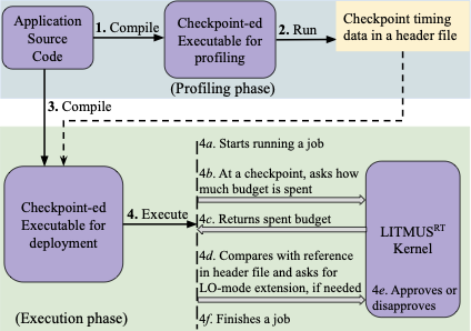
dynamically decides a program’s execution budget based on its runtime progress and theoretical analysis of the allowable delay at specific checkpoint locations. At runtime, measures the time (i.e., CPU time) to reach a checkpoint from the start of a task, and then compares that time to a pre-profiled reference value. The task’s execution budget which was previously set based on profiling, is then adjusted according to actual progress.
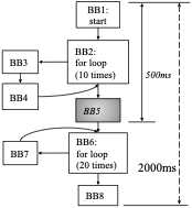
Figure 1 shows the CFG for a program with two loops, starting at BB2 and BB6. In this example, inserts a checkpoint between the two loops at the end of BB5. BB5 is a potentially good location for a checkpoint because there is one loop before and after this BB, providing an opportunity to increase the budget to compensate for the delay until BB5.
Suppose that we derive the LO-mode budget of the whole program to be 2000 ms by profiling, and the LO-mode time to reach the checkpoint at BB5 is 500 ms. The program is then executed in the presence of other tasks. The execution budget at the checkpoint (in BB5) is adjusted, to account for the program’s actual runtime progress. For example, suppose the program experiences a delay of $`100`$ ms to reach the checkpoint in BB5, thereby arriving at $`600`$ ms instead of the expected $`500`$ ms. Therefore, the program is delayed by ($`\frac{100}{500}\times 100`$=) 20% from its LO-mode progress.
 />
/>
Depending on the relationship between the task’s LO- and HI-mode progress to the checkpoint, the task’s budget is adjusted according to the 20% observed delay at the checkpoint. One approach is to extrapolate a linear delay from the checkpoint to the end of the task’s execution. Thus, the total execution time of 2000 ms is predicted to complete at ($`2000 + 20\% \times 2000`$=) 2400 ms. uses the available information at a checkpoint to extend the LO-mode budget of a high-criticality application. In Section 5.8, we explore other possible execution time prediction models.
Benefits of Adaptive Mixed-criticality Scheduling
We see progress-aware scheduling as being beneficial in mixed-criticality systems. Adaptive Mixed-criticality scheduling is the state-of-the-art fixed-priority scheduling policy for Mixed-criticality tasksets. In AMC, a system is first initialized to run in LO-mode. In LO-mode, all the tasks are executed with their LO-mode execution budgets. Whenever a high-criticality task overruns its LO-mode budget, the system is switched to HI-mode. In HI-mode, all low-criticality tasks are discarded (or given reduced execution time ), and the high-criticality tasks are given increased HI-mode budgets. The system’s switch to HI-mode therefore impacts the QoS for low-criticality tasks.
By combining with AMC (to yield AMC-), we extend the LO-mode budget of a high-criticality task to its predicted execution time at a checkpoint. Going back to our previous example in Figure 1, we try to extend the LO-mode budget of the task by 400 ms. We carry out an online schedulability test to determine if we can extend the task’s LO-mode budget by 400 ms. If the whole taskset is still schedulable after an extension of the LO-mode budget of the delayed high-criticality task, the increment in the task’s LO-mode budget is approved. We let the task run until the extended time and keep the system in LO-mode. In case the high-criticality task finishes within its extended time, we avoid an unnecessary switch to HI-mode. Thus, the low-criticality tasks run for an extended period of time and do not suffer from degraded CPU utilization and QoS, as occurs with AMC.
In case the task does not finish within the predicted time, then the system is changed to HI-mode, and low-criticality tasks are finally dropped. This behavior is identical to AMC, and every high-criticality task still finishes within its own deadline. Therefore, we improve the QoS of the low-criticality tasks when the high-criticality tasks finish within their extended LO-mode budgets, and otherwise, we fall back to AMC. When there is no delay at a checkpoint, we do not change a task’s LO-mode budget.
We tested our implementation of AMC and AMC- in with real-world applications on an Intel NUC Kit . The machine has an Intel Core i7-5557U 3.1GHz processor with 8GB RAM, running Linux kernel 4.9. We use three applications in our evaluations: a high-criticality object classification application from the Darknet neural network framework , a high-criticality object tracking application from dlib C++ library , and a low-criticality MPEG video decoder . These applications are chosen for their relevance to the sorts of applications that might be used in infotainment and autonomous driving systems. The dlib object tracking application is only used for the last set of experiments to test two different execution time prediction models.
For object classification, we use the COCO dataset images for both
profiling and execution. The dataset for the Profiling phase was chosen
from random images from the dataset and used to determine the LO- and
HI-mode budgets of the Darknet high-criticality application. The dataset
for the Execution phase was also randomly chosen but similarly
distributed in terms of image dimensions as the data of the Profiling
phase was. For the video decoder application, we use the Big Buck
Bunny video as the input. We have turned off memory locking with
mlock by the liblitmus library, as multiple object classification
tasks collectively require more RAM than the physical 8GB limit.
Task Parameters
Table [tab:amc_taskset] shows the LO- and HI-mode budgets for the three applications. Each object classification and tracking task consist of a series of jobs that classify objects in a single image. Each video decoder task decodes 30 frames in a single job.
| Application | C(LO) | C(HI) |
|---|---|---|
| Darknet object classification | 345 ms | 627 ms |
| dlib object tracking | 10.7 ms | 18 ms |
| video decoder | 250 ms | - |
The LO-mode budget, $`C(LO)`$, is the average time that a task takes to complete its job. In Section 5.5, we also present experiments where we increase our LO-mode budget estimate. The HI-mode budget, $`C(HI)`$, accounts for the worst-case running time of the high-criticality task for any of its jobs. The LO-mode utilization of each individual task is generated by the UUnifast algorithm . We then calculate a task’s period by dividing its LO-mode budget by its utilization.
In all experiments, we observed that none of the tasks exceed their HI-mode budget. Consequently, none of the high-criticality tasks miss their deadlines in any of our tests. Hence, we assume that our derivation of LO- and HI-mode budgets are safe and correct for our experiments. The main focus of our evaluation now is to compare the QoS of the LC tasks.
QoS Improvements for Low-criticality Tasks
We compare the QoS for low-criticality tasks using AMC and AMC- in different cases. In every case, each taskset has an equal number of high-criticality object classification tasks and low-criticality video decoder tasks. We experiment with ten schedulable tasksets in all cases except the base case described below. We run each of the tests ten times, and we report the average of the measurements for low-criticality tasks. As stated earlier, all high-criticality tasks meet their timing requirements in each case. Execution time prediction at a checkpoint for is done with a linear extrapolation model for all the experiments ($`f(C_i(LO), X) = C_i(LO) + \ddfrac{C_i(LO) \times X}{100}`$ from Section [sec:theory]) except in Section 5.8 where we discuss other approaches.
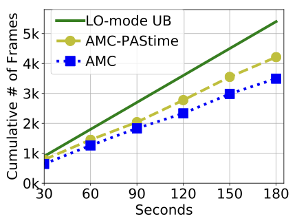
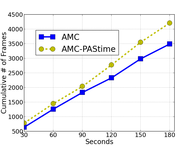
Our base case is to run one high-criticality object classification task and one low-criticality video decoder task for 180 seconds. Here, we set the periods of both tasks to 1000 ms rather than using the UUnifast algorithm, yielding a total LO-mode utilization of ~60%.
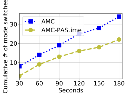
Figure 2 shows the cumulative number of frames decoded by the video decoder task. The LO-mode Upper Bound (UB) line shows the cumulative number of decoded frames if the system is kept in LO-mode all the time. This line represents a theoretical UB for a decoded frame playback rate of 30 frames per second over the entire experimental run.
We see in Figure 2 that AMC- has a 9–21% increase in the cumulative number of decoded frames compared to AMC scheduling. The performance of the low-criticality task is related to the number of HI-mode switches in the two scheduling policies. AMC- decreases the number of HI-mode switches by 35%, compared to AMC scheduling.
 style="width:97.0%" />
 style="width:99.0%" />
 style="width:99.0%" />
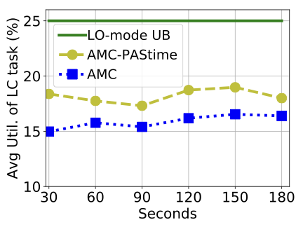
Although the number of decoded frames is an illustrative metric for a video decoder’s QoS, the average utilization of an application is a more generic metric. Average utilization represents the CPU share a task receives over a period of time. Figure 3 shows that AMC- achieves 10% more utilization on average for the video decoder task, compared to AMC scheduling. The LO-mode UB line is the maximum utilization of the video decoder task, which is 25% (i.e., $`C(LO)/Period`$ = 250 ms/1000 ms).
Scalability
To test system scalability, we increase the number of tasks in a taskset up to 20 tasks. As explained above, we generate the periods of the tasks by distributing the total LO-mode utilization of ~60% to all the tasks using the UUnifast algorithm. This setup is inspired by the theoretical parameters in previous mixed-criticality research work . The LO-mode utilization bound for low-criticality tasks remains between 25–35%.
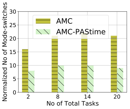
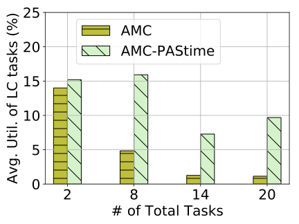
Figure 4 shows the average utilization of the low-criticality tasks, when the total tasks vary from 2 to 20. Each task in this case consists of 20 jobs. We see that the average utilization drops for AMC scheduling as the number of tasks increases.
AMC- achieves significantly greater average utilization for the low-criticality tasks, by deferring system switches to HI-mode until much later than with AMC scheduling. This is because the LO-mode budgets for the high-criticality tasks are extended due to runtime delays.
AMC- decreases the number of mode switches by 28–55%. AMC-’s resistance to switching into HI-mode allows low-criticality tasks to make progress. This in turn improves their QoS. In these experiments, AMC- improves the utilization of the low-criticality tasks by a factor of $`3`$, $`5`$ and $`9`$, respectively, for 8, 14 and 20 tasks. Table 5 shows that AMC- reduces the number of mode-switches compared to AMC.
Varying the Initial Total LO-mode Utilization
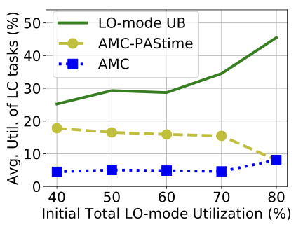
In this test, we vary the initial total LO-mode utilization for 8 tasks from 40% to 80% by adjusting the periods of all tasks. The initial utilization does not account for increases caused by LO-mode budget extensions to high-criticality tasks.
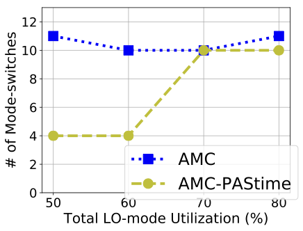
Figure [fig:util_amc_avg_lc_util] demonstrates that AMC- improves average utilization of the low-criticality tasks by more than 3 times, up to 70% total LO-mode utilization. After that, AMC- and AMC scheduling converge to the same average utilization for low-criticality tasks. This is because there is insufficient surplus CPU time in LO-mode for AMC- to accommodate the extended budget of a high-criticality task. Therefore, the LO-mode extension requests are disapproved by AMC-. The reduced number of mode switches for AMC-, shown in Table 6, also corroborates the rationale behind AMC-’s better performance than AMC.
We note that the schedulability of random tasksets decreases with higher LO-mode utilization in AMC scheduling. Therefore, many real-world tasksets may not be schedulable because of their HI-mode utilization. Thus, AMC-’s improved performance is significant for practical use-cases.
Estimation of LO-mode Budget
In our evaluations until now, we estimate a LO-mode budget based on the average execution time of the high-criticality object classification application. In the next set of experiments, we estimate the LO-mode budget of a high-criticality task to be a certain percentage above the average profiled execution time. An increased LO-mode budget for high-criticality tasks benefits AMC scheduling. This is because high-criticality tasks are now given more time to complete in LO-mode, and therefore low-criticality tasks will still be able to execute as well. As a result, the utilization of low-criticality tasks is able to increase.
Suppose that $`C(LO)`$ is an average execution time estimate for the LO-mode budget of a high-criticality task. Let $`(C(LO) + o)`$ be an overestimate of the LO-mode budget. As before, AMC- detects an $`X\%`$ lag at a checkpoint and predicts the total execution time to be $`C(LO) + e`$. If the actual LO-mode budget is $`(C(LO) + o)`$ then AMC- requests for an extra budget of $`(e-o)`$, assuming $`(e-o) > 0`$.
Even for overestimated $`C(LO)`$, Figure [fig:amc_overestimate] shows that AMC- still improves utilization for the low-criticality tasks by more than a factor of 3 up to an overestimation of 40%. Overestimation helps in reducing the number of mode switches for AMC scheduling after 40%, as high-criticality tasks have larger budgets in LO-mode.
There is no improvement by AMC scheduling after 60% LO-mode budget overestimation. AMC- also shows no benefits with increased overestimation, because the LO-mode budget extensions are disapproved by the online schedulability test. Therefore, the system is switched to HI-mode by an overrun of a high-criticality task.
 style="width:98.0%" />
 style="width:98.0%" />
 />
/>
Checkpoint Location
We use our modified LLVM compiler in the Profiling phase to determine a
viable checkpoint for the high-criticality object classification task.
We instrument checkpoints in the forward_network function of the
Darknet neural network module. We consider four checkpoint locations in
the Profiling phase, which are both automatically and manually
instrumented. In the Execution phase, we measure performance for each of
these checkpoint locations.
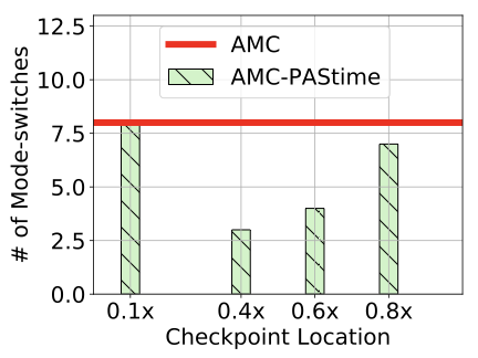
Figure 7 shows the variation
in the number of mode switches against the location of a checkpoint. The
x-axis is the approximated division point of a checkpoint location with
respect to $`C(LO)`$. For example, 0.1$`\times`$ means that the
checkpoint is at $`(0.1
\times
C(LO))`$.
We see that the number of mode switches decreases if the location of a checkpoint is more towards the middle of the code. However, a checkpoint near the start and the end of the source code have nearly the same number of mode switches, as with AMC scheduling. A checkpoint near the beginning of a program is not able to capture sufficient delay to increase the LO-mode budget enough to prevent a mode switch. Likewise, a checkpoint near the end of a program is often too late. A HI-mode switch may occur before the high-criticality task even reaches its checkpoint. Hence, a checkpoint at $`0.8\times`$ in the source code of a program reduces the number of mode switches by just 1.
Overheads
The main overheads of AMC- compared to AMC are the online schedulability test and budget extension. We first derive an upper bound on the overhead by offline analysis and compare with the experimental measurements.
Our offline upper bound is the total number of iterations in solving the response time recurrence relations during the schedulability test in AMC-. We generate 500 random tasksets of 20 tasks for different initial LO-mode utilizations. Initial LO-mode utilizations range from 40% to 90%. The utilization of each individual task is generated using the UUnifast algorithm, and each period is taken from 10 to 1000 simulated time units, as done in previous work . As our experimental taskset has a criticality factor (CF $`=\ddfrac{C(HI)}{C(LO)}`$) of ~1.8, we also test with a CF of $`1.8`$.
Among the schedulable tasks with AMC scheduling, we increase the demand in LO-mode budget of the highest priority task. Then, we calculate the total number of iterations needed to determine whether an extension of the budget can be approved by an offline version of the online schedulability test. Here, one iteration is a single update to the response time in any one of the recurrence equations (in Equations [eq:LO_AMC_Online] and [eq:HC_AMC_Star_Online]) used to test for schedulability.
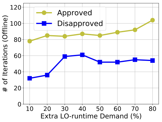
We increase the demand for extra budget from 10 to 80% in this analysis because the CF is $`1.8`$. We check the maximum number of iterations to decide the schedulability of a taskset across the 500 tasksets. We carry out this offline analysis with 40-90% initial LO-mode utilization.
In Figure [fig:offline_iterations], we show the maximum number of iterations to decide the schedulability of a taskset, against a demand of 10 to 80% extra budget in LO-mode by the highest priority task. Each point in the figure represents the maximum iterations across the 500 tasksets to either approve or disapprove of schedulability.
We have observed the number of iterations to be as high as $`120`$. Therefore, we set 120 as the highest number of allowed iterations for the online schedulability test. When the number of iterations exceed 120 at runtime, we disapprove a LO-mode budget extension. This strategy maintains a safe and known upper bound on the online overhead of AMC-.
 style="width:95.0%" />
 style="width:98.0%" />
 />
/>
Microbenchmarks
Each iteration of a response time calculation has a worst-case time of
1$`\mu`$s, for our implementation of the online schedulability test in .
Therefore, we bound the worst-case delay for the online schedulability
test in at 120$`\mu`$s for our test cases. Additionally, the worst-case
execution time for the ANNOUNCE_TIME macro is 10$`\mu`$s. Hence, the
maximum total overhead of an ANNOUNCE_TIME call, accounting for the
schedulability test, is 130$`\mu`$s. The 130$`\mu`$s overhead is
factored into the LO-mode extension inside the kernel.
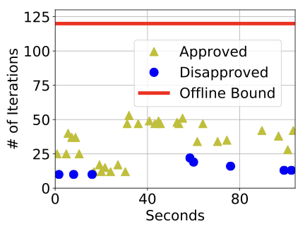
Figure [fig:iterations] shows the number of iterations for the online schedulability test for a taskset of 20 tasks with 60% initial total LO-mode utilization, in cases where an extension was approved and disapproved. We see that the offline bound of 120 iterations is much higher than the actually observed number of iterations. Hence, we never need to abandon the schedulability test because of excessive overheads. In addition, disapproval takes less time than approval online, which corroborates our offline observations in Figure [fig:offline_iterations].
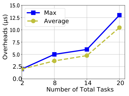
Figure 8 shows the maximum and average times for a LO-mode budget extension decision including the online schedulability test. It demonstrates that the extension approval decision takes more time with increasing number of tasks. However, the maximum times are still significantly lower than the offline upper bound of 130$`\mu`$s for 20 tasks. In general, budget extension overheads can be bounded according to the number of tasks in the system.
Execution Time Prediction Model
As we have explained in Section [sec:theory], the execution time after a checkpoint is predicted by a function $`f(C_i(LO), X)`$, where $`C_i(LO)`$ is the LO-mode budget, and $`X\%`$ is the observed delay percentage relative to the LO-mode time to reach the checkpoint. The parameter $`X`$ in $`f`$ is a timing progress metric, which is used to make runtime scheduling decisions in .
Linear Extrapolated Delay
We have already shown in the previous experiments how a straightforward linear extrapolated delay improves the utilization of LC tasks compared to AMC for an object classification application. In such a case, $`f(C_i(LO), X) = C_i(LO)
- \frac{C_i(LO) \times X}{100}`$. A linear extrapolation of delay at a checkpoint applied to the entire LO-mode time makes sense in the absence of additional knowledge that could influence the remaining execution time of the task.
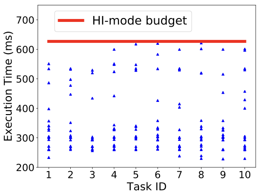
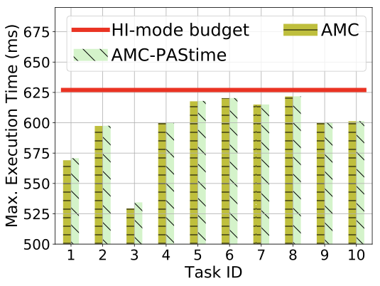
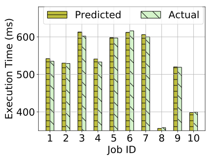
We now investigate further whether the linear extrapolation is effective in detecting the amount of delay in our Darknet high-criticality object classification task. We compare the predicted and actual times taken by the high-criticality tasks when LO-mode is extended by AMC-. This experiment is performed with 8 tasks for 40 jobs each. The initial total LO-mode utilization is 60%, before applying budget extensions.
We show ten of the extended jobs in Figure [fig:amc_pastime_prediction]. We see that the predicted execution times are close to the actual execution times. For cases where the predicted times exceed the actual budget expenditure, the predictions overestimate execution by just 0.88% on average for this experiment. In Figure [fig:amc_pastime_prediction], Job ID 6, 8 and 10 show lower predicted times than the actual spent budgets. For these jobs, the system is switched to HI-mode because the extended LO-mode is not enough for a task to complete its job. In these cases, the predicted times are smaller than the spent budgets by 0.49%.
This experiment shows that the checkpoint is effectively being used to predict the execution time of a high-criticality task in most cases. The budget extensions are a reasonable estimate of the actual task requirements.
 style="width:99.0%" />
 style="width:94.0%" />
 />
/>
Alternative Execution Time Compensation Models
In our experiments, we compare the linear extrapolation model with an alternative compensatory execution time prediction model. The alternative approach compensates for the observed delay at a checkpoint, by adding the delay amount to the predicted execution time. If the observed delay is $`Y`$, then the estimated total execution time is $`C^\prime_i(LO) = C_i(LO) + Y`$.
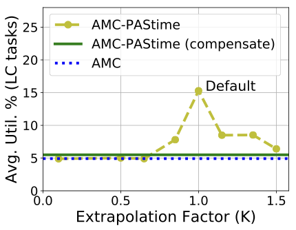
We have also investigated variations to the linear extrapolation model, even though it has proven effective in our previous experiments. A further experiment multiplies the extrapolated delay by a factor $`K`$, such that the predicted execution time is $`f(C_i(LO), X) = C_i(LO) + K \times \ddfrac{C_i(LO) \times X}{100}`$.
Figure [fig:linear_extrapolation]
compares AMC- with the alternative compensatory model compensate, and
linear extrapolation model where $`K`$ ranges from 0.1 to 1.5. The
linear extrapolation model ($`K=1`$) outperforms the other approaches,
while the compensatory model improves the utilization slightly compared
to AMC.
Prediction based on Memory Access Time
Memory accesses by different processes compete for shared cache lines and consequently cause unexpected microarchitectural delays. There are previous works that model the memory and cache accesses in a multicore machine to deal with the issue of predictable execution. Here, we demonstrate with an execution time prediction model based on the number of memory accesses, to increase the LO-mode budget of a high-criticality task.
In this model, we note the number of memory accesses by a high-criticality task as we measure the LO- and HI-mode execution time of the task during the Profiling phase. We measure the average number of memory accesses in LO-mode for each profiled run of a task with different inputs, and denote it by $`M(LO)`$.
During the Profiling phase, we also measure the number of memory accesses in LO-mode before and after a checkpoint: $`M_{\text{pre\_}CP}(LO), M_{\text{post\_}CP}(LO)`$. These values are also averaged across all runs of a given task. Therefore, $`M_{\text{pre\_}CP}(LO) + M_{\text{post\_}CP}(LO) = M(LO)`$
We define a new memory instructions progress metric to be the ratio of task execution time to the number of memory accesses. The LO-mode value of this metric is $`Pr_{mem, LO} = \frac{C(LO)}{M(LO)}`$.
In the Execution phase, we measure the number of memory accesses and the used budget up to a checkpoint, respectively denoted by $`M_{CP}`$ and $`C_{used}`$ for a given task. During Execution, we calculate the memory instructions progress metric at a checkpoint, $`Pr_{mem, CP} = \frac{C_{used}}{M_{CP}}`$. If $`Pr_{mem, CP} \le Pr_{mem, LO}`$, we predict the task is progressing as expected in LO-mode in terms of memory access-related delays. There are other factors such as I/O-related delays that affect the execution time of a task. However, I/O should be budgeted separately from the main task, as shown in prior work for AMC . Notwithstanding, is capable of supporting even richer prediction models based on a multitude of factors that cause delays due to microarchitectural and task interference overheads.
When $`Pr_{mem, CP} > Pr_{mem, LO}`$, we predict a task’s memory access delays. We calculate the expected number of memory instructions after a checkpoint: $`M_{\text{expected_post_CP}}
\frac{M_{CP} \times
M_{\text{post_CP}}(LO)}{M_{\text{pre_}CP}(LO)}$, and increase the LO-mode budget by $(M_{\text{expected_post_}CP}
\times (Pr_{mem, CP}$ - $Pr_{mem, LO}))`$. This increment helps cover
future memory delays after a checkpoint.
We tested both high-criticality dlib object tracking and Darknet object
classification applications with this model.
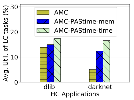
Figure 9 shows experimental results
with 4 HC tasks (either dlib or Darknet) and 4 LC video decoder tasks,
with initial 50% LO-mode utilization. We see that AMC--mem with this
memory access progress metric provides better utilization to the LC
tasks than AMC. However, it is not better than AMC--time, which uses
the default linear extrapolated execution time prediction. Nevertheless,
the result shows that some form of progress metric dynamically improves
the utilization of LC tasks.
This paper presents , a scheduling strategy based on the execution progress of a task. Progress is measured by observing the time taken for a program to reach a designated checkpoint in its control flow graph (CFG). We integrate in mixed-criticality systems by extending AMC scheduling. extends the LO-mode budget of a high-criticality task based on its observed progress, given that the extension does not violate the schedulability of any tasks. Our extension to AMC scheduling, called AMC-, is shown to improve the QoS of low-criticality tasks. Moreover, we implement an algorithm in the LLVM compiler to automatically detect and instrument viable program checkpoints for use in task profiling.
While both meet deadlines for all high-criticality tasks, AMC- improves the average utilization of low-criticality tasks by 1.5–9 times for 2–20 total tasks. AMC- is shown to improve performance for low-criticality tasks while reducing the number of mode switches. Finally, we have shown that different progress metrics also improve the LC tasks’ utilization.
In future work, we will explore other uses of progress-aware scheduling
in timing-critical systems. We plan to extend the Linux kernel
SCHED_DEADLINE policy to support progress-aware scheduling. We
believe that is applicable to timing-sensitive cloud computing
applications, where it is possible to adjust power (e.g., via Dynamic
Voltage Frequency Scaling) based on progress. Application of to domains
outside real-time computing will also be considered in future work.
Over-estimation of worst-case execution times (WCETs) of real-time tasks leads to poor resource utilization. In a mixed-criticality system (MCS), the over-provisioning of CPU time to accommodate the WCETs of highly critical tasks may lead to degraded service for less critical tasks. In this paper we present , a novel approach to monitor and adapt the runtime progress of highly time-critical applications, to allow for improved service to lower criticality tasks. In , CPU time is allocated to time-critical tasks according to the delays they experience as they progress through their control flow graphs. This ensures that as much time as possible is made available to improve the Quality-of-Service of less critical tasks, while high-criticality tasks are compensated after their delays.
This paper describes the integration of with Adaptive Mixed-criticality (AMC) scheduling. The LO-mode budget of a high-criticality task is adjusted according to the delay observed at execution checkpoints. We observe in our experimental evaluation that AMC- significantly improves the utilization of the low-criticality tasks while guaranteeing service to high-criticality tasks.
In this section, we provide a response time analysis for AMC- by extending the analysis for AMC scheduling. We also describe details about the online schedulability test based on the response time values.
Task Model
We use the same AMC task model as described by Baruah et al . Without loss of generality, we restrict ourselves to two criticality levels - LO and HI. Each task, $`\tau_i`$, has five parameters: $`C_i(LO)`$ - LO-mode runtime budget, $`C_i(HI)`$ - HI-mode runtime budget, $`D_i`$ - deadline, $`T_i`$ - period, and $`L_i`$ - criticality level of a task, which is either high ($`HC`$) or low ($`LC`$). We assume each task’s deadline, $`D_i`$, is equal to its period, $`T_i`$. A HC task has two budgets: $`C_i(LO)`$ for LO-mode assurance and $`C_i(HI)~(> C_i(LO))`$ for HI-mode assurance. A LC task has only one budget of $`C_i(LO)`$ for LO-mode assurance.
Scheduling Policy
Both AMC and AMC- use the same task priority ordering, based on Audsley’s priority assignment algorithm . If a task’s response time for a given priority order is less than its period, then the task is deemed schedulable. The details of the priority assignment strategy are discussed in previous research work . We do not change the priority ordering of the tasks at runtime.
AMC- initializes a system in LO-mode with all tasks assigned their LO-mode budgets. We extend a high-criticality task’s LO-mode budget at a checkpoint if the task is lagging behind its expected progress, as long as the extension does not hamper the schedulability of the delayed task and all the lower or equal priority tasks. An increase to the LO-mode budget of a task that violates its own or other task schedulability is not allowed. If a high-criticality task has not finished its execution even after its extended LO-mode budget, then the system is switched to HI-mode.
Response Time Analysis
The AMC response time recurrence equations for (1) all tasks in LO-mode, (2) HC tasks in HI-mode, and (3) HC tasks during mode-switches are shown in Equation [eq:LO_AMC], [eq:HC_HI_AMC] and [eq:HC_AMC_Star], respectively. $`hp(i)`$ is the set of tasks with priorities higher than or equal to that of $`\tau_i`$. Likewise, $`hpHC(i)`$ and $`hpLC(i)`$ are the set of high- and low-criticality tasks, respectively, with priorities higher than or equal to the priority of $`\tau_i`$.
AMC provides two analyses for mode switches: AMC-response-time-bound (AMC-rtb) and AMC-maximum. We use AMC-rtb for our analysis, as AMC-maximum is computationally more expensive. However, AMC-rtb does not allow a taskset which is not schedulable by AMC-maximum. Therefore, AMC-rtb is sufficient for schedulability.
\begin{equation}
\begin{aligned}
R_i^{LO} = C_i (LO) + \sum_{\tau_j \in hp(i)} \ceil{\frac{R_i^{LO}}{T_j}}
\times
C_j (LO)
\label{eq:LO_AMC}
\end{aligned}
\end{equation}\begin{equation}
\begin{aligned}
R_i^{HI} = C_i (HI) + \sum_{\tau_j \in hpHC(i)} \ceil{\frac{R_i^{HI}}{T_j}}
\times C_j (HI)
\label{eq:HC_HI_AMC}
\end{aligned}
\end{equation}\begin{equation}
\begin{aligned}
R_i^{*} = C_i (HI) &+ \sum_{\tau_j \in hpHC(i)} \ceil{\frac{R_i^{*}}{T_j}}
\times C_j (HI)
&+ \sum_{\tau_j \in hpLC(i)} \ceil{\frac{R_i^{LO}}{T_j}}
\times C_j (LO)
\label{eq:HC_AMC_Star}
\end{aligned}
\end{equation}With AMC-, we not only measure $`C_i(LO)`$ and $`C_i(HI)`$, but also the LO-mode time to reach a checkpoint $`C_i^{CP}(LO)`$. If a high-criticality task, $`\tau_i`$, is delayed by $`X\%`$ at a checkpoint, compared to its LO-mode progress, then $`\tau_i`$ takes $`(C_i^{CP}(LO) + \frac{C_i^{CP}(LO) \times X}{100})`$ time to reach the checkpoint. Hence, $`\tau_i`$’s budget is tentatively increased from $`C_i(LO)`$ to $`C_i^\prime(LO)`$, where $`C_i^\prime(LO) = f(C_i(LO), X)`$. Here, $`f(C_i(LO), X)`$ is a function to predict the delayed total execution time, given that the observed delay until the checkpoint is $`X\%`$. For example, by a linear extrapolation of the observed delay of $`X\%`$ at a checkpoint, the original budget $`C_i(LO)`$ changes to $`f(C_i(LO), X) = \big(C_i(LO) + \ddfrac{C_i(LO) \times X}{100}\big)`$. It is possible for $`f`$ to depend on task-specific and hardware microarchitectural factors such as cache and main memory accesses. We show more execution time prediction techniques in Section 5.8.
With the increased LO-mode budget $`C_i^\prime(LO)`$, an online schedulability test then calculates the the extended LO-mode response time, $`R_i^{LO{\text{-ext}}}`$, for $`\tau_i`$, using Equation [eq:LO_AMC_Online]. Similarly, $`R_i^{*{\text{-ext}}}`$ is calculated using Equation [eq:HC_AMC_Star_Online]. Equations [eq:LO_AMC_Online] and [eq:HC_AMC_Star_Online] are extensions of Equations [eq:LO_AMC] and [eq:HC_AMC_Star]. AMC- checks at runtime whether both $`R_i^{LO{\text{-ext}}}`$ and $`R_i^{*{\text{-ext}}}`$ are less than or equal to $`\tau_i`$’s period to determine its schedulability.
The new response times are then calculated for all tasks in LO-mode with priorities less than or equal to $`\tau_i`$, using Equation [eq:LO_AMC_Online]. Similarly, new response times are calculated for all HC tasks with lower or equal priority to $`\tau_i`$ during a mode switch, using Equation [eq:HC_AMC_Star_Online]. If all newly calculated response times are less than or equal to the respective task periods, the system is schedulable. In this case, AMC- approves the LO-mode budget extension to $`\tau_i`$. If the system is not schedulable, then $`\tau_i`$’s budget remains $`C_i(LO)`$.
\begin{equation}
\begin{aligned}
R_i^{LO{\text{-ext}}} = C_i^\prime (LO) &+ \sum_{\tau_j \in hp(i)}
\ceil{\frac{R_i^{LO{\text{-ext}}}}{T_j}}
\times C_j^\prime (LO)
\label{eq:LO_AMC_Online}
\end{aligned}
\end{equation}\begin{equation}
\begin{aligned}
R_i^{*{\text{-ext}}} = C_i (HI) &+ \sum_{\tau_j \in hpHC(i)}
\ceil{\frac{R_i^{*{\text{-ext}}}}{T_j}}
\times C_j (HI)
&+ \sum_{\tau_j \in hpLC(i)} \ceil{\frac{R_i^{LO{\text{-ext}}}}{T_j}}
\times C_j (LO)
\label{eq:HC_AMC_Star_Online}
\end{aligned}
\end{equation}AMC- only extends the LO-mode budget of a delayed HC task for its current job. When a new job for the same HC task is dispatched, it starts with its original LO-mode budget. If another request for an extension in LO-mode for the same task appears, AMC- tests the schedulability with the maximum among the requested extended budgets. The system keeps track of the maximum extended budget for a task and uses that value for online schedulability testing. We explain the AMC- scheduling scheme with an example taskset in Table 1.
| Task | Type | C(LO) | C(HI) | T | Pr | $`R^{LO}`$ | $`R^*`$ |
|---|---|---|---|---|---|---|---|
| $`\tau_1`$ | HC | 3 | 6 | 10 | 1 | 3 | 6 |
| $`\tau_2`$ | LC | 2 | - | 9 | 2 | 5 | - |
| $`\tau_3`$ | HC | 5 | 10 | 50 | 3 | 15 | 38 |
A Mixed-criticality Taskset Example
Suppose, task $`\tau_1`$ is delayed by 66% at a checkpoint in the task’s source code. will then try to extend the budget by $`(3\times\frac{66}{100})\approx 2`$ time units. Therefore, the potential extended budget $`C_1^\prime(LO)`$ for $`\tau_1`$ would be $`(3+2)=5`$ time units. will calculate the response times, $`R_i^{LO\text{-ext}}`$ and $`R_i^{*\text{-ext}}`$, for $`\tau_1`$ and the lower priority tasks $`\tau_2`$ and $`\tau_3`$. $`R_1^{LO{\text{-ext}}}`$ would just be 5, and $`R_1^{*{\text{-ext}}}`$ would remain the same as $`R_1^*=6`$, as $`\tau_1`$ is the highest priority task. The new $`R_2^{LO{\text{-ext}}}`$ would be 7 (by Equation [eq:LO_AMC_Online]) which is smaller than its period of 9. Therefore, $`\tau_2`$ would still be schedulable if we extend $`\tau_1`$’s LO-mode budget from 3 to 5.
For $`\tau_3`$, the new $`R_3^{LO{\text{-ext}}}`$ and $`R_3^{*{\text{-ext}}}`$ would be, respectively, 26 (by Equation [eq:LO_AMC_Online]) and 40 (by Equation [eq:HC_AMC_Star_Online]) which are also smaller than $`\tau_3`$’s period of 50. Therefore, the extended budget of $`5`$ for $`\tau_1`$ would be approved by AMC-. In conventional AMC scheduling, the system would be switched to HI-mode if $`\tau_1`$ did not finish within 3 time units. However, AMC- will extend $`\tau_1`$’s LO-mode budget to 5 because of the observed delay at its checkpoint, so the system is kept in LO-mode. Consequently, LC task $`\tau_2`$ is allowed to run by AMC-, if $`\tau_1`$ finishes before 5 time units. If $`\tau_1`$ does not finish even after 5 time units, the system would be switched to HI-mode.
In this example, 5 jobs of $`\tau_1`$ are dispatched for every single job of $`\tau_3`$, as $`\tau_3`$’s period of 50 is 5 times the period of $`\tau_1`$. Suppose $`\tau_1`$ asks for the 66% increment in its LO-mode budget for the first job, as we have explained above. In its second job, $`\tau_1`$ asks for an increment of 33% (1 time unit) in its LO-mode budget. In this case, we again need to calculate the response times for all tasks. If we calculate the online response times for $`\tau_2`$ and $`\tau_3`$ assuming $`(3+1)=4`$ time units for $`C_1^\prime(LO)`$, then we would not account for the first job of $`\tau_1`$, which potentially executes for 5 time units. We would need to keep track of the extended LO-mode budgets for all jobs of $`\tau_1`$, to accurately calculate online response times for $`\tau_2`$ and $`\tau_3`$.
To avoid the cost of recording all extended LO-mode budgets for a task,
AMC- simply stores the maximum extended budget for a task. When
calculating online response times to check whether to approve an
extension to the LO-mode budget, the system uses the maximum extended
budget of every high-criticality task. This value is stored in the
max_extended_budget variable for each HC task. Therefore, when
$`\tau_1`$ asks for $`4`$ time units as its extended LO-mode budget in
its second job, the system calculates $`R_1^{LO{\text{-ext}}}`$,
$`R_1^{*{\text{-ext}}}`$, $`R_2^{LO{\text{-ext}}}`$,
$`R_3^{LO{\text{-ext}}}`$, $`R_3^{*{\text{-ext}}}`$ with
$`C_1^\prime(LO)=5`$.
AMC- uses maximum extended budgets to calculate safe upper bounds for
online response times. The max_extended_budget task property is reset
when a task has not requested a LO-mode budget extension for any of its
dispatched jobs within the maximum period of all tasks.
Online Schedulability Test
AMC- performs an online schedulability test whenever a high-criticality task asks for an extension to its LO-mode budget. The test calculates the response times ($`R_i^{LO\text{-ext}}`$ and $`R_i^{*\text{-ext}}`$) of the delayed high-criticality task and all lower priority tasks. Then, it checks whether the response times are less than or equal to the task periods. If any task’s response time is greater than its period, the online schedulability test returns false, and the extension in LO-mode for the high-criticality task is denied. If the schedulability test is successful the high-criticality task is permitted to run for its extended budget in LO-mode.
Input: $`tasks`$ - set of all tasks in priority order $`\tau_k`$ - delayed task $`e`$ - extra budget for $`\tau_k`$ Output: $`true`$ or $`false`$ $`e^\prime`$ = max$`(\tau_k.`$max_extended_budget$`, C_k(LO)+e)- C_k(LO)`$ $`C_i^\prime(LO) = \tau_i.`$max_extended_budget $`C_i^\prime(LO) =`$max$`(C_i^\prime(LO), C_i(LO) + e)`$ Initialize $`R_i^{LO{\text{-ext}}}`$ for Equation 4 with $`R_i^{LO} + e^\prime`$ Solve Equation 4 Initialize $`R_i^{*{\text{-ext}}}`$ for Equation 4 with $`R_i^{*}`$ Solve Equation 5 with the new $`R_i^{LO{\text{-ext}}}`$ Return $`false`$ Return $`false`$ $`\tau_k.`$max_extended_budget = max($`C_k(LO) + e, \tau_k.`$max_extended_budget) Return $`true`$
Algorithm [algo:change_budget_runtime] shows the pseudocode for the online schedulability test. The offline response time values ($`R_i^{LO}`$ and $`R_i^{*}`$) are stored in the properties for each task $`\tau_i`$. When a high-criticality task $`\tau_k`$ is delayed, it asks for an extension of its LO-mode budget by $`e`$ time units.
Line [lst:line:new_e_max] in
Algorithm [algo:change_budget_runtime]
determines whether the newly requested extension, $`e`$, is more than a
previously saved maximum extended budget for $`\tau_k`$. In
lines [lst:line:max_budget_start]–[lst:line:max_budget_end],
the $`C_i^\prime(LO)`$ is set to the maximum extended budget for all the
lower priority tasks and $`\tau_k`$. As we have explained above, it is
practically infeasible to store the execution times of every job of all
the tasks to calculate online response times. Therefore, we store the
maximum extended budget of every task and use this to calculate response
times online. For the currently delayed task, $`\tau_k`$,
$`C_k^\prime(LO)`$ is set to the maximum value between a previously
saved max_extended_budget and the currently requested $`C_k(LO) + e`$.
Considering the example in
Table 1 from the paper,
line [lst:line:c_i_dash_low] would
translate to $`C_i^\prime(LO)`$=max(5, 4) for the second LO-mode
extension request.
Then, Equation 4 is solved in line [lst:line:eq_lo_amc_online] by initializing $`R_i^{LO\text{-ext}}`$ to the $`R_i^{LO}`$ plus extra budget $`e^\prime`$ from line [lst:line:new_e_max]. If a lower priority task is a high-criticality task, then $`R_i^{*\text{-ext}}`$ is calculated in line [lst:line:solve_hc_amc], with the newly derived value of $`R_i^{LO\text{-ext}}`$.
Online response time calculations may take significant time, depending on the number of iterations of Equations [eq:LO_AMC_Online] and [eq:HC_AMC_Star_Online]. However, the response time values from Equations [eq:LO_AMC], [eq:HC_HI_AMC], [eq:HC_AMC_Star] are already calculated offline to determine the schedulability of a taskset using Audsley’s priority assignment algorithm with AMC scheduling. Since AMC- uses the same priority ordering as AMC, the offline response times for schedulability remain the same.
AMC- initializes the online $`R_i^{LO\text{-ext}}`$ in Equation [eq:LO_AMC_Online] with $`R_i^{LO} + e`$, where $`R_i^{LO}`$ is calculated offline by Equation [eq:LO_AMC] and $`e(>0)`$ is the extra budget of the delayed task.
Since the budget of a delayed task is extended by $`e`$, $`R_i^{LO\text{-ext}}`$ must be greater than or equal to $`R_i^{LO} + e`$. Hence, this is a good initial value to start calculating $`R_i^{LO\text{-ext}}`$ online. In Section [sec:evaluation], we establish an upper bound on the total number of iterations needed to check the schedulability of random tasksets, if the highest priority task’s budget is extended by different amounts.
📊 논문 시각자료 (Figures)


![]()