- Title: Training DNN IoT Applications for Deployment On Analog NVM Crossbars
- ArXiv ID: 1910.13850
- Date: 2020-10-19
- Authors: Fernando Garc ia-Redondo, Shidhartha Das, Glen Rosendale
📝 Abstract
A trend towards energy-efficiency, security and privacy has led to a recent focus on deploying DNNs on microcontrollers. However, limits on compute and memory resources restrict the size and the complexity of the ML models deployable in these systems. Computation-In-Memory architectures based on resistive nonvolatile memory (NVM) technologies hold great promise of satisfying the compute and memory demands of high-performance and low-power, inherent in modern DNNs. Nevertheless, these technologies are still immature and suffer from both the intrinsic analog-domain noise problems and the inability of representing negative weights in the NVM structures, incurring in larger crossbar sizes with concomitant impact on ADCs and DACs. In this paper, we provide a training framework for addressing these challenges and quantitatively evaluate the circuit-level efficiency gains thus accrued. We make two contributions: Firstly, we propose a training algorithm that eliminates the need for tuning individual layers of a DNN ensuring uniformity across layer weights and activations. This ensures analog-blocks that can be reused and peripheral hardware substantially reduced. Secondly, using NAS methods, we propose the use of unipolar-weighted (either all-positive or all-negative weights) matrices/sub-matrices. Weight unipolarity obviates the need for doubling crossbar area leading to simplified analog periphery. We validate our methodology with CIFAR10 and HAR applications by mapping to crossbars using 4-bit and 2-bit devices. We achieve up to 92:91% accuracy (95% floating-point) using 2-bit only-positive weights for HAR. A combination of the proposed techniques leads to 80% area improvement and up to 45% energy reduction.
💡 Summary & Analysis
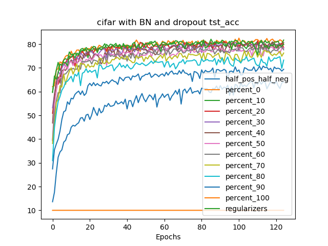
This paper introduces a training framework to address the challenges of deploying deep learning networks (DNNs) on analog non-volatile memory (NVM)-based crossbars. It aims to enable high-performance DNN execution in systems with limited computational and memory resources, such as microcontrollers. The authors propose two main contributions: firstly, they suggest a training algorithm that ensures uniformity across layer weights and activations without the need for tuning individual layers, which allows analog blocks to be reused and reduces peripheral hardware requirements substantially. Secondly, using neural architecture search (NAS) methods, they recommend unipolar-weighted matrices or sub-matrices, either all-positive or all-negative, which eliminate the need for doubling crossbar area and simplify analog periphery.
The paper evaluates its methodology by mapping DNNs to crossbars with 4-bit and 2-bit devices on datasets like CIFAR10 and HAR applications. The results show up to 92:91% accuracy using only positive 2-bit weights for the HAR application, demonstrating significant improvements in both area (80%) and energy consumption (up to 45%).
This work is crucial as it provides a pathway towards deploying complex DNNs on resource-constrained systems. By enabling efficient execution of high-performance models on devices like microcontrollers, this research can significantly impact IoT applications, where low power and high performance are critical.
📄 Full Paper Content (ArXiv Source)
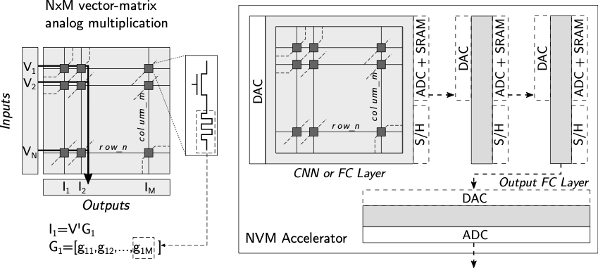
# Hard-Constrained HW Quantized Training
To address the reconfigurability versus full-custom periphery design,
and its dependence on the weights/activation precision, we have
developed a framework to aid mapping the DNN to the NVM hardware at
training time. The main idea behind it is the use of hard-constraints
when computing forward and back-propagation passes. These constraints,
related to the HW capabilities, impose the precision used on the
quantization of each layer, and guarantee that the weight, bias and
activation values that each layer can have are shared across the NN.
This methodology allows, after the training is finished, to map each
hidden layer $`L_i`$ to uniform HW blocks sharing:
a single DAC/ADC design performing $`\mathcal{V}()`$ / $`act()`$
a single weight-to-conductance mapping function $`f()`$
a global set of activation values $`Y_g = [y_0, y_1]`$
a global set of input values $`X_g = [x_0, x_1]`$
a global set of weight values $`W_g = [w_0, w_1]`$
and every system variable within the sets $`Y_g, X_g, W_g`$ and $`B_g`$,
every DAC/ADC performing $`\mathcal{V}()`$ and $`act()`$ will share
design and can potentially be reused. To achieve the desired behavior we
need to ensure at training time that the following equations are met for
each hidden layer $`L_i`$ present in the NN:
Commonly, the output layer activation (sigmoid, softmax) does not
match the hidden layers activation. Therefore for the DNN to learn the
output layer should be quantized using an independent set of values
$`Y_o, X_o, W_o, B_o`$ that may or not match $`Y_g, X_g, W_g, B_g`$.
Consequently, the output layer is the only layer that once mapped to the
crossbar requires full-custom periphery.
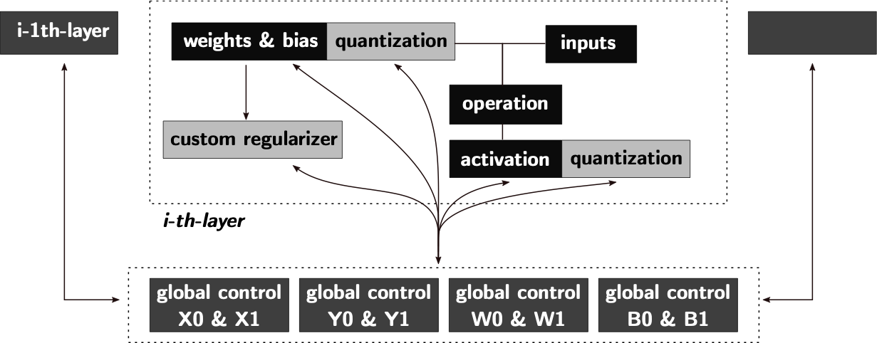
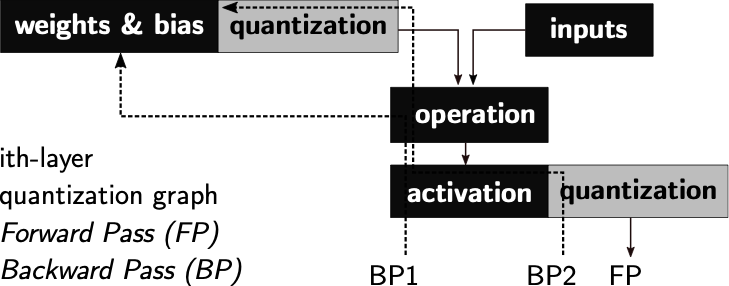
HW Aware Graph Definition
/>
Simplified version of the proposed quantized graph for
crossbar-aware training, automatically handling the global variables
involved in the quantization process, achieving uniform scaling across
layers.
The NN graphs are generated by Tensorflow Keras libraries. In order to
perform the HW-aware training, elements controlling the quantization,
accumulation clippings, and additional losses, are added to the graph.
Figure 1 describes these
additional elements, denoted as global variables. For this purpose,
the global variable control blocks manage the definition, updating and
later propagation of the global variables. A global variable is a
variable used to compute a global set of values $`V_g`$ composed of the
previously introduced $`Y_g, X_g, W_g, B_g`$ or others. Custom
regularizer blocks may also be added to help the training to converge
when additional objectives are present.
HW Aware NN Training
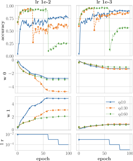
Differentiable Architecture and Variables Updating During Training
Each global variable can be non-updated during training, –fixing the
value of the corresponding global set in $`V_g`$– or dynamically
controlled using the related global variable control. If fixed, a
design space exploration is required in order to find the best set of
global variable hyperparameters for the given problem. On the
contrary, we propose the use of a Differentiable Architecture (DA) to
automatically find the best set of global variable values using the
back-propagation. In order to do that, we make use of DA to explore the
NN design space. To achieve it, we define the global variables as a
function of each layer characteristics –mean, max, min, deviations, etc.
If complying with DA requirements, the global control elements
automatically update the related variables descending through the
gradient computed in the back-propagation stage. On the contrary, should
a specific variable not be directly computable by the gradient descent,
it would be updated in a later step as depicted in
algorithm [alg:darts].
Set of global variables $`V_g = \{X_g, Y_g, W_g, B_g\}`$ Initialize
$`V_g`$ Update weights $`W`$ Compute non-differentiable vars in $`V_g`$
Update layer quantization parameters
We also propose the use of DA on the definition of inference networks
that target extremely low precision layers (i.e. $`2`$ bit weights and
$`2-4`$ bits in activations), to explore the design space, and to find
the most suitable activation functions to be shared across the network
hidden layers. In
Section 12 experiments we explore the use
(globally, in every hidden layer) of a traditional relu versus a
customized tanh defined as $`tanh(x - th_g)`$. Our NN training is able
to choose the most appropriate activation, as well as to find the
optimal parameter $`th_g`$. The parameter $`th_g`$ is automatically
computed through gradient descent. However, to determine which kind of
activation to use, we first define the continuous activations design
space as
which forces either $`a_0`$ or $`a_1`$ to a $`0`$ value once the
training converges .
Loss Definition
As introduced before, additional objectives/constraints related to the
final HW characteristics may lead to non convergence issues (see
Section 4.3). In order to help the
convergence towards a valid solution, we introduce extra
$`\mathcal{L}_C`$ terms in the loss computation that may depend on the
training step. The final loss $`\mathcal{L}_F`$ is then defined as
where $`\mathcal{L}`$ refers the standard training loss,
$`\{\mathcal{L}_{L1}, \mathcal{L}_{L2}\}`$ refer the standard $`L1`$ and
$`L2`$ regularization losses, and $`\mathcal{L}_C`$ is the custom
penalization. An example of this particular regularization terms may
refer the penalization of weight values beyond a threshold $`W_T`$ after
training step $`N`$. This loss term can be formulated as
where $`\alpha_C`$ is a preset constant and $`HV`$ the Heaviside
function. If the training would still provide weights whose values
surpass $`W_T`$, $`HV`$ function can be substituted by a non clipped
function $`relu(step-N)`$. In particular, this $`\mathcal{L}_C`$
function was used in the unipolarity experiments located at
Section 12.
Implemented Quantization Scheme
The implemented quantization stage takes as input a random tensor
$`T = \{t_t\}, t_t \in \mathbb{R}`$ and projects it to the quantized
space $`Q = \{q_{q+}, q_{q-}\}`$, where $`q_{q+} = \alpha_Q 2^{q}`$,
$`q_{q-} = -\alpha_Q 2^{q}`$, and $`\alpha \in \mathbb{R}`$. Therefore
the projection is denoted as $`q(T) = T_q`$, where
$`T_q = \{t_q\}, t_q \in Q`$. For its implementation we use fake_quant
operations computing straight through estimator as the quantization
scheme, which provides us with the uniformly distributed $`Q`$ set,
always including $`0`$. However, the quantization nodes shown in
Figure 1 allow the use of
non-uniform quantization schemes. The definition of the quantized space
$`Q`$ gets determined by the minimum and maximum values given by the
global variables $`V_g`$.
Algorithm [alg:darts] can consider either
$`max/min`$ functions or stochastic quantization schemes . Similarly,
the quantization stage is dynamically activated/deactivated using the
global variable $`do_Q \in {0, 1}`$, with could be easily substituted to
support incremental approaches . In particular, and as shown in
Section 4.3, the use of
alpha-blending scheme proves useful when the weight precision is very
limited.
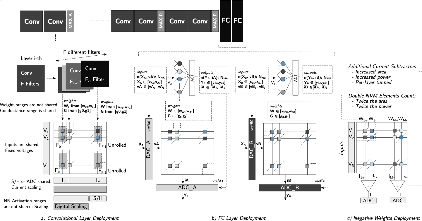
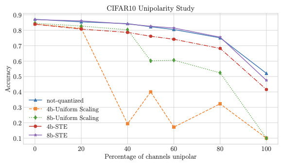
Unipolar Weight Matrices Quantized Training
Mapping positive/negative weights to the same crossbar involve double
the crossbar resources and introducing additional periphery. Using the
proposed training scheme we can restrict further the characteristics of
the DNN graph obtaining unipolar weight matrices, by redefining some
global variables as
MATH
\begin{equation}
W_g  \in [0, w_1]
\end{equation}
Click to expand and view more
and introducing the $`\mathcal{L}_C`$ function defined by
Equation [eq:loss_c].
Moreover, for certain activations (relu, tanh, etc.) the maximum
and/or minimum values are already known, and so the sets of parameters
in $`V_g`$ can be constrained even further. These maximum and minimum
values can easily be mapped to specific parameters in the activation
function circuit interfacing the crossbar . Finally, in cases where
weights precision is very limited (i.e. $`2`$ bits), additional loss
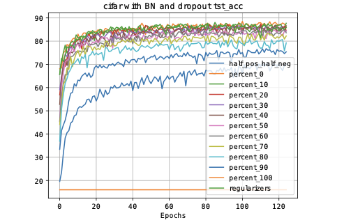
terms as $`\mathcal{L}_C`$ gradually move weight distributions from a
bipolar space to an only positive space, helping the training to
converge.
In summary, by applying the mechanisms described in
Section 4, we open the possibility of
obtaining NN graphs only containing unipolar weights.
The copyright of this content belongs to the respective researchers. We deeply appreciate their hard work and contribution to the advancement of human civilization.