Optimizing Loss Functions Through Multivariate Taylor Polynomial Parameterization

Introduction
As deep learning systems have become more complex, their architectures and hyperparameters have become increasingly difficult and time-consuming to optimize by hand. In fact, many good designs may be overlooked by humans with prior biases. Therefore, automating this process, known as metalearning, has become an essential part of the modern machine learning toolbox. Metalearning aims to solve this problem through a variety of approaches, including optimizing different aspects of the architecture from hyperparameters to topologies, and by using different methods from Bayesian optimization to evolutionary computation .
Recently, loss-function discovery and optimization has emerged as a new type of metalearning. Focusing on neural network’s root training goal it aims to discover better ways to define what is being optimized. However, loss functions can be challenging to optimize because they have a discrete nested structure as well as continuous coefficients. The first system to do so, Genetic Loss Optimization tackled this problem by discovering and optimizing loss functions in two separate steps: (1) representing the structure as trees, and evolving them with Genetic Programming ; and (2) optimizing the coefficients using Covariance-Matrix Adaptation Evolutionary Strategy . While the approach was successful, such separate processes make it challenging to find a mutually optimal structure and coefficients. Furthermore, small changes in the tree-based search space do not always result in small changes in the phenotype, and can easily make a function invalid, making the search process ineffective.
In an ideal case, loss functions would be mapped into arbitrarily long, fixed-length vectors in a Hilbert space. This mapping should be smooth, well-behaved, well-defined, incorporate both a function’s structure and coefficients, and should by its very nature exclude large classes of infeasible loss functions. This paper introduces such an approach: Multivariate Taylor expansion-based genetic loss-function optimization (TaylorGLO). With a novel parameterization for loss functions, the key pieces of information that affect a loss function’s behavior are compactly represented in a vector. Such vectors are then optimized for a specific task using CMA-ES. Special techniques can be developed to narrow down the search space and speed up evolution.
Loss functions discovered by TaylorGLO outperform the standard cross-entropy loss (or log loss) on the MNIST, CIFAR-10, and SVHN datasets with several different network architectures. They also outperform the Baikal loss, discovered by the original GLO technique, and do it with significantly fewer function evaluations. The reason for the improved performance is that evolved functions discourage overfitting to the class labels, thereby resulting in automatic regularization. These improvements are particularly pronounced with reduced datasets where such regularization matters the most. TaylorGLO thus further establishes loss-function optimization as a promising new direction for metalearning.
Related work
Applying deep neural networks to new tasks often involves significant manual tuning of the network design. The field of metalearning has recently emerged to tackle this issue algorithmically . While much of the work has focused on hyperparameter optimization and architecture search, recently other aspects, such activation functions and learning algorithms, have been found useful targets for optimization . Since loss functions are at the core of machine learning, it is compelling to apply metalearning to their design as well.
Deep neural networks are trained iteratively, by updating model parameters (i.e., weights and biases) using gradients propagated backward through the network . The process starts from an error given by a loss function, which represents the primary training objective of the network. In many tasks, such as classification and language modeling, the cross-entropy loss (also known as the log loss) has been used almost exclusively. While in some approaches a regularization term is added to the the loss function definition, the core component is still the cross-entropy loss. This loss function is motivated by information theory: It aims to minimize the number of bits needed to identify a message from the true distribution, using a code from the predicted distribution.
In other types of tasks that do not fit neatly into a single-label classification framework different loss functions have been used successfully . Indeed, different functions have different properties; for instance the Huber Loss is more resilient to outliers than other loss functions. Still, most of the time one of the standard loss functions is used without a justification; therefore, there is an opportunity to improve through metalearning.
Genetic Loss Optimization provided an initial approach into metalearning of loss functions. As described above, GLO is based on tree-based representations with coefficients. Such representations have been dominant in genetic programming because they are flexible and can be applied to a variety of function evolution domains. GLO was able to discover Baikal, a new loss function that outperformed the cross-entropy loss in image classification tasks. However, because the structure and coefficients are optimized separately in GLO, it cannot easily optimize their interactions. Many of the functions created through tree-based search are not useful because they have discontinuities, and mutations can have disproportionate effects on the functions. GLO’s search is thus inefficient, requiring large populations that are evolved for many generations.
The technique presented in this paper, TaylorGLO, aims to solve these problems through a novel loss function parameterization based on multivariate Taylor expansions. Furthermore, since such representations are continuous, the approach can take advantage of CMA-ES as the search method, resulting in faster search.
Loss Functions as Multivariate Taylor expansions
Taylor expansions are a well-known function approximator that can represent differentiable functions within the neighborhood of a point using a polynomial series. Below, the common univariate Taylor expansion formulation is presented, followed by a natural extension to arbitrarily-multivariate functions.
Given a $`C^{k_{\text{max}}}`$ smooth (i.e., first through $`k_{\text{max}}`$ derivatives are continuous), real-valued function, $`f(x): \mathbb{R}\to\mathbb{R}`$, a $`k`$th-order Taylor approximation at point $`a\in \mathbb{R}`$, $`\hat{f}_k(x,a)`$, where $`0\leq k \leq k_{\text{max}}`$, can be constructed as
\begin{equation}
\hat{f}_k(x,a) = \sum_{n=0}^k \frac{1}{n!} f^{(n)}(a) (x-a)^n    .
\end{equation}
Conventional, univariate Taylor expansions have a natural extension to arbitrarily high-dimensional inputs of $`f`$. Given a $`C^{k_{\text{max}+1}}`$ smooth, real-valued function, $`f(\vec{x}): \mathbb{R}^n\to\mathbb{R}`$, a $`k`$th-order Taylor approximation at point $`\vec{a}\in \mathbb{R}^n`$, $`\hat{f}_k(\vec{x},\vec{a})`$, where $`0\leq k \leq k_{\text{max}}`$, can be constructed. The stricter smoothness constraint compared to the univariate case allows for the application of Schwarz’s theorem on equality of mixed partials, obviating the need to take the order of partial differentiation into account.
Let us define an $`n`$th-degree multi-index, $`\alpha = (\alpha_1,\alpha_2,\ldots,\alpha_n)`$, where $`\alpha_i \in \mathbb{N}_0`$, $`|\alpha| = \sum_{i=1}^n \alpha_i`$, $`\alpha! = \prod_{i=1}^n \alpha_i!`$. $`\vec{x}^\alpha = \prod_{i=1}^n x_i^{\alpha_i}`$, and $`\vec{x} \in \mathbb{R}^n`$. Multivariate partial derivatives can be concisely written using a multi-index
\begin{equation}
\partial^\alpha f = \partial_1^{\alpha_1}\partial_2^{\alpha_2}\cdots\partial_n^{\alpha_n} f = \frac{\partial^{|\alpha|}}{\partial x_1^{\alpha_1}\partial x_2^{\alpha_2}\cdots\partial x_n^{\alpha_n}}   .
\end{equation}
Thus, discounting the remainder term, the multivariate Taylor expansion for $`f(\vec{x})`$ at $`\vec{a}`$ is
\begin{equation}
\hat{f}_k(\vec{x},\vec{a}) = \sum_{\forall \alpha,|\alpha|\leq k} \frac{1}{\alpha!} \partial^{\alpha}f(\vec{a}) (\vec{x}-\vec{a})^\alpha    .
\end{equation}
The unique partial derivatives in $`\hat{f}_k`$ and $`\vec{a}`$ are parameters for a $`k`$th order Taylor expansion. Thus, a $`k`$th order Taylor expansion of a function in $`n`$ variables requires $`n`$ parameters to define the center, $`\vec{a}`$, and one parameter for each unique multi-index $`\alpha`$, where $`|\alpha|\leq k`$. That is: $`\#_{\text{parameters}}(n,k) = n + {n+k\choose k} = n + \frac{(n+k)!}{n!\,k!}`$.
The multivariate Taylor expansion can be leveraged for a novel loss-function parameterization. Let an $`n`$-class classification loss function be defined as $`\mathcal{L}_{\text{Log}} = -\frac{1}{n}\sum^{n}_{i=1} f(x_i,y_i)`$. The function $`f(x_i,y_i)`$ can be replaced by its $`k`$th-order, bivariate Taylor expansion, $`\hat{f}_k(x,y,a_x,a_y)`$. More sophisticated loss functions can be supported by having more input variables beyond $`x_i`$ and $`y_i`$, such as a time variable or unscaled logits. This approach can be useful, for example, to evolve loss functions that change as training progresses.
For example, a loss function in $`\vec{x}`$ and $`\vec{y}`$ has the following third-order parameterization with parameters $`\vec{\theta}`$ (where $`\vec{a} = \left< \theta_0, \theta_1 \right>`$):
\begin{equation}
\label{eq:k3example}
\begin{aligned}
\mathcal{L}(\vec{x},\vec{y}) = -\frac{1}{n}\sum^n_{i=1} \Big[      \theta_2 + \theta_3(y_i -\theta_1)+ \tfrac{1}{2}\theta_4(y_i -\theta_1)^2 + \tfrac{1}{6}\theta_5(y_i -\theta_1)^3 + \theta_6(x_i -\theta_0)\\[-0.6em]
   + \theta_7(x_i -\theta_0)(y_i -\theta_1)+ \tfrac{1}{2}\theta_8(x_i -\theta_0)(y_i -\theta_1)^2 + \tfrac{1}{2}\theta_9(x_i -\theta_0)^2 \\
   + \tfrac{1}{2}\theta_{10}(x_i -\theta_0)^2(y_i -\theta_1)+ \tfrac{1}{6}\theta_{11}(x_i -\theta_0)^3  \Big]
\end{aligned}
\end{equation}
Notably, the reciprocal-factorial coefficients can be integrated to be a part of the parameter set by direct multiplication if desired.
As will be shown in this paper, the technique makes it possible to train neural networks that are more accurate and learn faster than those with tree-based loss function representations. Representing loss functions in this manner confers several useful properties:
-
It guarantees smooth functions;
-
Functions do not have poles (i.e., discontinuities going to infinity or negative infinity) within their relevant domain;
-
They can be implemented purely as compositions of addition and multiplication operations;
-
They can be trivially differentiated;
-
Nearby points in the search space yield similar results (i.e., the search space is locally smooth), making the fitness landscape easier to search;
-
Valid loss functions can be found in fewer generations and with higher frequency;
-
Loss function discovery is consistent and not dependent on a specific initial population; and
-
The search space has a tunable complexity parameter (i.e., the order of the expansion).
These properties are not necessarily held by alternative function approximators. For instance:
are well suited for approximating periodic functions . Consequently, they are not as well suited for loss functions, whose local behavior within a narrow domain is important. Being a composition of waves, Fourier series tend to have many critical points within the domain of interest. Gradients fluctuate around such points, making gradient descent infeasible. Additionally, close approximations require a large number of terms, which in itself can be injurious, causing large, high-frequency fluctuations known as “ringing”, due to Gibb’s phenomenon .
can be more accurate approximations than Taylor expansions; indeed, Taylor expansions are a special case of Padé approximants where $`M = 0`$ . However, unfortunately Padé approximants can model functions with one or more poles, which valid loss functions typically should not have. These problems still exist, and are exacerbated, for Chisholm approximants and Canterbury approximants .
can represent functions with discontinuities, the simplest being $`x^{-1}`$. While Laurent polynomials provide a generalization of Taylor expansions into negative exponents, the extension is not useful because it results in the same issues as Padé approximants.
can represent continuous functions within a finite domain, however, the number of parameters is prohibitive in multivariate cases.
The multivariate Taylor expansion is therefore a better choice than the alternatives. It makes it possible to optimize loss functions efficiently in TaylorGLO, as will be described next.
The TaylorGLO method
r0.44
TaylorGLO (Figure [fig:overview]) aims to find the optimal parameters for a loss function represented as a multivariate Taylor expansion. The parameters for a Taylor approximation (i.e., the center point and partial derivatives) are referred to as $`\vec{\theta}_{\hat{f}}`$: $`\vec{\theta}_{\hat{f}} \in \Theta`$, $`\Theta = \mathbb{R}^{\#_{\text{parameters}}}`$. TaylorGLO strives to find the vector $`\vec{\theta}_{\hat{f}}^*`$ that parameterizes the optimal loss function for a task. Because the values are continuous, as opposed to discrete graphs of the original GLO, it is possible to use continuous optimization methods.
In particular, Covariance Matrix Adaptation Evolutionary Strategy is a popular population-based, black-box optimization technique for rugged, continuous spaces. CMA-ES functions by maintaining a covariance matrix around a mean point that represents a distribution of solutions. At each generation, CMA-ES adapts the distribution to better fit evaluated objective values from sampled individuals. In this manner, the area in the search space that is being sampled at each step grows, shrinks, and moves dynamically as needed to maximize sampled candidates’ fitnesses. TaylorGLO uses the ($`\mu/\mu,\lambda`$) variant of CMA-ES , which incorporates weighted rank-$`\mu`$ updates to reduce the number of objective function evaluations needed.
In order to find $`\vec{\theta}_{\hat{f}}^*`$, at each generation CMA-ES samples points in $`\Theta`$. Their fitness is determined by training a model with the corresponding loss function and evaluating the model on a validation dataset. Fitness evaluations may be distributed across multiple machines in parallel and retried a limited number of times upon failure. An initial vector of $`\vec{\theta}_{\hat{f}} = \vec{0}`$ is chosen as a starting point in the search space to avoid bias.
Fully training a model can be prohibitively expensive in many problems. However, performance near the beginning of training is usually correlated with performance at the end of training, and therefore it is enough to train the models only partially to identify the most promising candidates. This type of approximate evaluation is common in metalearning . An additional positive effect is that evaluation then favors loss functions that learn more quickly.
For a loss function to be useful, it must have a derivative that depends on the prediction. Therefore, internal terms that do not contribute to $`\frac{\partial}{\partial \vec{y}}\mathcal{L}_f(\vec{x},\vec{y})`$ can be trimmed away. This step implies that any term $`t`$ within $`f(x_i,y_i)`$ with $`\frac{\partial}{\partial y_i}t = 0`$ can be replaced with $`0`$. For example, this refinement simplifies Equation [eq:k3example], providing a reduction in the number of parameters from twelve to eight:
\begin{equation}
\label{eq:k3taylorglo}
\vspace{-1em}
\begin{aligned}
\mathcal{L}(\vec{x},\vec{y}) = -\frac{1}{n}\sum^n_{i=1} \Big[    \theta_2(y_i -\theta_1)+ \tfrac{1}{2}\theta_3(y_i -\theta_1)^2 + \tfrac{1}{6}\theta_4(y_i -\theta_1)^3 + \theta_5(x_i -\theta_0)(y_i -\theta_1)\\[-1em]
 + \tfrac{1}{2}\theta_6(x_i -\theta_0)(y_i -\theta_1)^2 + \tfrac{1}{2}\theta_7(x_i -\theta_0)^2(y_i -\theta_1)\Big] \;.
\end{aligned}
\end{equation}
Experimental setup
This section presents the experimental setup that was used to evaluate the TaylorGLO technique.
Domains: MNIST was included as simple domain to illustrate the method and to provide a backward comparison with GLO; CIFAR-10 and SVHN were included as more modern benchmarks. Improvements were measured in comparison to the standard cross-entropy loss function $`\mathcal{L}_{\text{Log}} = -\frac{1}{n}\sum^{n}_{i=1} x_i \log (y_i),`$ where $`x`$ is sampled from the true distribution, $`y`$ is from the predicted distribution, and $`n`$ is the number of classes.
Evaluated architectures: A variety of architectures were used to evaluate TaylorGLO: the basic CNN architecture evaluated in the GLO study , AlexNet , AllCNN-C , Preactivation ResNet-20 , which is an improved variant of the ubiquitous ResNet architecture , and Wide ResNets of different morphologies . Networks with Cutout were also evaluated, to show that TaylorGLO provides a different approach to regularization.
TaylorGLO setup: CMA-ES was instantiated with population size $`\lambda=28`$ on MNIST and $`\lambda=20`$ on CIFAR-10, and an initial step size $`\sigma=1.2`$. These values were found to work well in preliminary experiments. The candidates were third-order (i.e., $`k=3`$) TaylorGLO loss functions (Equation [eq:k3taylorglo]). Such functions were found experimentally to have a better trade-off between evolution time and performance compared to second- and fourth-order TaylorGLO loss functions, although the differences were relatively small.
Further experimental setup and implementation details are provided in Appendix 21.
Results
| Task and Model | Avg. TaylorGLO Acc. | Avg. Baseline Acc. | $`p`$-value |
|---|---|---|---|
| MNIST on Basic CNN | 0.9951 (0.0005) | 0.9899 (0.0003) | 2.95 |
| CIFAR-10 on AlexNet | 0.7901 (0.0026) | 0.7638 (0.0046) | 1.76 |
| CIFAR-10 on PreResNet-20 | 0.9169 (0.0014) | 0.9153 (0.0021) | 0.0400 |
| CIFAR-10 on AllCNN-C | 0.9271 (0.0013) | 0.8965 (0.0021) | 0.42 |
| CIFAR-10 on AllCNN-C + Cutout | 0.9329 (0.0022) | 0.8911 (0.0037) | 1.60 |
| CIFAR-10 on Wide ResNet 16-8 | 0.9558 (0.0011) | 0.9528 (0.0012) | 1.77 |
| CIFAR-10 on Wide ResNet 16-8 + Cutout | 0.9618 (0.0010) | 0.9582 (0.0011) | 2.55 |
| CIFAR-10 on Wide ResNet 28-5 | 0.9548 (0.0015) | 0.9556 (0.0011) | 0.0984 |
| CIFAR-10 on Wide ResNet 28-5 + Cutout | 0.9621 (0.0013) | 0.9616 (0.0011) | 0.1882 |
| SVHN on Wide ResNet 16-8 | 0.9658 (0.0007) | 0.9597 (0.0006) | 1.94 |
| SVHN on Wide ResNet 16-8 + Cutout | 0.9714 (0.0010) | 0.9673 (0.0008) | 9.10 |
| SVHN on Wide ResNet 28-5 | 0.9657 (0.0009) | 0.9634 (0.0006) | 6.62 |
| SVHN on Wide ResNet 28-5 + Cutout | 0.9727 (0.0006) | 0.9709 (0.0006) | 2.96 |
Test-set accuracy of loss functions discovered by TaylorGLO compared with that of the cross-entropy loss. The TaylorGLO results are based on the loss function with the highest validation accuracy during evolution. All averages are from ten separately trained models and $`p`$-values are from one-tailed Welch’s $`t`$-Tests. Standard deviations are shown in parentheses. TaylorGLO discovers loss functions that perform significantly better than the cross-entropy loss in almost all cases, including those that include Cutout, suggesting that it provides a different form of regularization.
Network architecture references:
r0.43
This section illustrates the TaylorGLO process and demonstrates how the evolved loss functions can improve performance over the standard cross-entropy loss function, especially on reduced datasets. A summary of results on three datasets across a variety of models are shown in Table 1.
The TaylorGLO discovery process
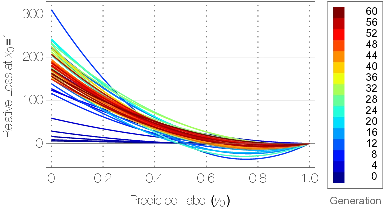
Figure [fig:mnist_evolution] illustrates the evolution process over 60 generations, which is sufficient to reach convergence on the MNIST dataset. TaylorGLO is able to discover highly-performing loss functions quickly, i.e. within 20 generations. Generations’ average validation accuracy approaches generations’ best accuracy as evolution progresses, indicating that population as a whole is improving. Whereas GLO’s unbounded search space often results in pathological functions, every TaylorGLO training session completed successfully without any instabilities.
Figure 1 shows the shapes and parameters of each generation’s highest-scoring loss function. In Figure 1$`a`$ the functions are plotted as if they were being used for binary classification, i.e. the loss for an incorrect label on the left and for a correct one on the right . The functions have a distinct pattern through the evolution process. Early generations include a wider variety of shapes, but they later converge towards curves with a shallow minimum around $`y_0=0.8`$. In other words, the loss increases near the correct output—which is counterintuitive. This shape is also strikingly different from the cross-entropy loss, which decreases monotonically from left to right, as one might expect all loss functions to do. The evolved shape is effective most likely because can provide an implicit regularization effect: it discourages the model from outputting unnecessarily extreme values for the correct class, and therefore makes overfitting less likely . This is a surprising finding, and demonstrates the power of machine learning to create innovations beyond human design.
(a) Best discovered
functions over time
(a) Best function
parameters over time
Performance comparisons
Over 10 fully-trained models, the best TaylorGLO loss function achieved a mean testing accuracy of 0.9951 (stddev 0.0005) in MNIST. In comparison, the cross-entropy loss only reached 0.9899 (stddev 0.0003), and the “BaikalCMA” loss function discovered by GLO, 0.9947 (stddev 0.0003) ; both differences are statistically significant (Figure [fig:mnist_accuracies]). Notably, TaylorGLO achieved this result with significantly fewer generations. GLO required 11,120 partial evaluations (i.e., 100 individuals over 100 GP generations plus 32 individuals over 35 CMA-ES generations), while the top TaylorGLO loss function only required 448 partial evaluations, i.e. $`4.03\%`$ as many. Thus, TaylorGLO achieves improved results with significantly fewer evaluations than GLO.
Such a large reduction in evaluations during evolution allows TaylorGLO to tackle harder problems, including models that have millions of parameters. On the CIFAR-10 and SVHN datasets, TaylorGLO was able to outperform cross-entropy baselines consistently on a variety models, as shown in Table 1. It also provides further improvement on architectures that use Cutout , suggesting that its mechanism of avoiding overfitting is different from other regularization techniques.
In addition, TaylorGLO loss functions result in more robust trained models. In Figure 2, accuracy basins for two AllCNN-C models, one trained with the TaylorGLO loss function and another with the cross-entropy loss, are plotted along a two-dimensional slice $`[-1,1]`$ of the weight space . The TaylorGLO loss function results in a flatter, lower basin. This result suggests that the model is more robust, i.e. its performance is less sensitive to small perturbations in the weight space, and it also generalizes better .


(a) Accuracy (b) Evaluations
Performance on reduced datasets
The performance improvements that TaylorGLO provides are especially pronounced with reduced datasets. For example, Figure 3 compares accuracies of models trained for 20,000 steps on different portions of the MNIST dataset (similar results were obtained with other datasets and architectures). Overall, TaylorGLO significantly outperforms the cross-entropy loss. When evolving a TaylorGLO loss function and training against $`10\%`$ of the training dataset, with 225 epoch evaluations, TaylorGLO reached an average accuracy across ten models of 0.7595 (stddev $`0.0062`$). In contrast, only four out of ten cross-entropy loss models trained successfully, with those reaching a lower average accuracy of $`0.6521`$. Thus, customized loss functions can be especially useful in applications where only limited data is available to train the models, presumably because they are less likely to overfit to the small number of examples.
Discussion and future work
TaylorGLO was applied to the benchmark tasks using various standard architectures with standard hyperparameters. These setups have been heavily engineered and manually tuned by the research community, yet TaylorGLO was able to improve them. Interestingly, the improvements were more substantial with wide architectures and smaller with narrow and deep architectures such as the Preactivation ResNet. While it may be possible to further improve upon this result, it is also possible that loss function optimization is more effective with architectures where the gradient information travels through fewer connections, or is otherwise better preserved throughout the network. An important direction of future work is therefore to evolve both loss functions and architectures together, taking advantage of possible synergies between them.
As illustrated in Figure 1$`a`$, the most significant effect of evolved loss functions is to discourage extreme output values, thereby avoiding overfitting. It is interesting that this mechanism is apparently different from other regularization techniques such as dropout and data augmentation with Cutout (as seen in Table 1). Dropout and Cutout improve performance over the baseline, and loss function optimization improves it further. This result suggests that regularization is a multifaceted process, and further work is necessary to understand how to best take advantage of it.
Another important direction is to incorporate state information into TaylorGLO loss functions, such as the percentage of training steps completed. TaylorGLO may then find loss functions that are best suited for different points in training, where, for example, different kinds of regularization work best . Unintuitive changes to the training process, such as cycling learning rates , have been found to improve performance; evolution could be used to find other such opportunities automatically. Batch statistics could help evolve loss functions that are more well-tuned to each batch; intermediate network activations could expose information that may help tune the function for deeper networks like ResNet. Deeper information about the characteristics of a model’s weights and gradients, such as that from spectral decomposition of the Hessian matrix , could assist the evolution of loss functions that adapt to the current fitness landscape. The technique could also be adapted to models with auxiliary classifiers as a means to touch deeper parts of the network.
Conclusion
This paper proposes TaylorGLO as a promising new technique for loss-function metalearning. TaylorGLO leverages a novel parameterization for loss functions, allowing the use of continuous optimization rather than genetic programming for the search, thus making it more efficient and more reliable. TaylorGLO loss functions serve to regularize the learning task, outperforming the standard cross-entropy loss significantly on MNIST, CIFAR-10, and SVHN benchmark tasks with a variety of network architectures. They also outperform previously loss functions discovered in prior work, while requiring many fewer candidates to be evaluated during search. Thus, TaylorGLO results in higher testing accuracies, better data utilization, and more robust models, and is a promising new avenue for metalearning.